44
The Stability of Coefficients in an Irish
Inter-Industry Model
By J McGILVRAY
{read before the Society on March 19th, 1965)
INTRODUCTION
This paper forms part of a study of mter-industry relations in Ireland, based upon the transactions table for 1956 compiled by the Central Statistics Office, and completed in 1961 1 One version of this Table is
reproduced here as Appendix I
It may be helpful to preface the main part of this paper by a brief discussion of the transactions table and the derived input-output model It is convenient to adopt the usual notation and divide the Table into four numbered quadrants, as indicated by the double lines in the Table Quadrant I, the top right-hand quadrant, shows "final" or "autonomous" demands upon the system of activities, in the Irish Table distinguished as Household current expenditure, Government current expenditure, Government capital expenditure, "Other" capital expenditure, Stock changes and Exports There is also a (negative) column of competitive imports, of which more in a moment (It should be noted that the alloca-tion of different rows and columns of transacalloca-tions to different quadrants depends upon the assumptions involved in the derived input-output model, in a "closed" model, for example, all transactions are regarded as "intermediate" and Quadrant I disappears as a separate quadrant)
Quadrant II, the mam part of the Table, records intermediate trans-actions between the producing sectors of the economy Thus each row records the sales of each industry to all other industries, and each column shows the purchases of each industry from all others These transactions form the statistical basis from which the input coefficients are derived,
1 The transactions table was kindly made available to me by Dr M D McCarthy,
45
and the size of this quadrant (in terms of number of sectors) normally determines the number of equations of the model and the size of the inverse matrix In the Irish Table, which is relatively small, thirty-six producing sectors are distinguished.
Quadrant III includes all direct factor (1 e "primary") inputs, here shown as wage and salaries, profits (including depreciation) and rent, also included are indirect taxes less subsidies, and non-competitive imports Finally, in Quadrant IV—the bottom right-hand section of the Table— there are a few miscellaneous entries including, inter aha, non-competitive imports sold direct to final demands, corresponding indirect taxes less subsidies, and factor incomes from abroad.
For each industry, total input=total output, in value terms This is ensured by the inclusion of profits as an input and net changes in stocks as an output The value of output of each industry consists of costs of materials and services bought from other industries or imported plus value added by the industry itself (including profits) Indirect taxes less subsidies are also added so that output is valued at what might be des-cribed as "sellers' market prices" This output is then sold to other industries (including mtra-mdustry sales) or to final buyers (including stock changes)
Without going into great detail on the construction of the Table, there are several features of the Input-Output Table which should be par-ticularly noted All transactions which cover the calendar year 1956 are recorded at current 1956 prices, and are net of distributive margins That is, the sale of an industry's output to other industries or to final demands does not include the distributive margin on such sales Instead, the dis-tributive margin is included as a separate purchase (from the industry "Distribution and Transport") by the purchasing industry or final buyer This means that each industry's input from "distribution and transport" refers to the distributive margin on purchases, not on sales A trans-actions table so prepared is said to be recorded on a producers' or sellers' prices basis
Some transactions tables are prepared on the basis of buyers' or pur-chasers' prices On this basis the sale of each industry's output to all others, and to final buyers, includes the distributive margin on sales Thus m the transactions table each industry's purchase of distribution and transport services refers to the distributive margin on sales, not on pur-chases Although a transactions table based on purchasers' prices is usually easier to prepare, the sellers' price system is normally preferred Briefly, the argument m favour of the latter is that the distributive margin on purchases is likely to be more stable than the distributive margin on sales, since sellers' margins tend to vary according to the destination of sales, e g the margin on sales to final buyers may ,be higher than that on intermediate sales, etc If this is the case than an input-output model derived from a table of transactions at sellers' prices is better, in terms of stability of input coefficients, than one derived from a table of trans-actions at purchasers' prices
46
transactions between establishments in the same sector 2 These mtra-sector sales are recorded in the main diagonal of Quadrant IT Tn some tables intra-sector sales are "netted-out", resulting in a diagonal of zero entries, in the Irish Table this was thought undesirable, principally because there is a high degree of aggregation of productive activities in the Table (In fact intra-sector sales accounted for over one-sixth of all intermediate sales)
A third point of particular interest concerns the treatment of imports in the transactions table—a problem which we consider in greater detail in Part II of this paper A distinction is made in the Table between im-ports which are competitive with domestic supplies and imim-ports which are regarded as non-competitive or complementary3 Imports of the latter type appear as a single row in Quadrant III (continued into Quadrant IV to include finished non-competitive products) as inputs into the purchasing sectors Included m this group are raw materials and semi-processed goods not available from domestic sources, and imported for further processing
Competitive imports are distributed along the rows of the Table with competing domestic supplies The total of such competitive imports, for each sector, is shown in Quadrant I of the Table The inclusion of com-petitive imports along the rows of the Table means that the rows of the Table show the distribution of total supplies of each "product",4 whether of domestic origin or imported, whilst the corresponding columns of the Table show the total of goods of domestic origin only Hence in order that the total outputs the total input for each sector, the column of competitive imports in Quadrant I contains negative entries The equality between total input and total output for each sector, therefore, is in terms of gross domestic outputs
In another version of the transactions table, not reproduced here, domestic supplies and competing imports are distinguished m greater detail Imports and domestic supplies are distributed separately along the rows of the Table, e g the "cell" showing sales of agricultural produce (Sector I) to the milling and animal food sector (Sector 5) contains three entries £13 501m of domestic produce, £3 597m of competitive imports and an aggregate figure of £17 098m for total sales In the Table only the aggregate figure is recorded Further reference to this treatment, how-ever, will be made in Part II
Much of the initial work on the transactions table involved a com-parison and reconciliation of the input-output accounts and the national
2 In most of the subsequent discussion we use the word "sector" rather than
"industry", which latter term may imply a somewhat narrower classification of activities than is in fact the case in the Table
3 We ignore here the difficulty in distinguishing between competitive and
non-competitive imports in many cases, though this point is discussed m Part II
4 The term "product" is used here as a convenient shorthand to described the
47
income accounts and other official data This particular aspect of the study is excluded from the present paper but is relevant to mention in so fan as the input-output accounts correspond with the national income accounts, in terms of such aggregates as GNP, imports and exports, wages and salaries, demand categories, etc
The transactions table described above and reproduced in the Appendix forms the statistical basis for the derivation of an "input-output model" A number of distinct types of model can be formed on the basis of any one transactions table, and within the framework of the following dis-cussion the type of model employed here is the simple, open, static type in which all final demand categories in Quadrant I are regarded as exogenous It is perhaps useful to elaborate this statement, by briefly outlining the assumptions underlying this model
The transactions table is a record of the flow of goods and services between different sectors of the economy over a specific time period (usually one year) Although measured in money values, it is convenient to regard all transactions as physical units of output, expressed—for purposes of homogeneity—in constant unit values Now consider the distribution of the output of any one sector—say sector 1 Part of sector I'S output is disposed of to final demands, e g personal consumption, exports, etc , the level of which is assumed to be "given" or exogenous. The remainder of sector I'S output is sold to other sectors, as part of those sectors' input It is assumed that the sale of product 1 to any other sector j is a unique function of sector j's output It is furthermore assumed that this function is linear in form Thus, if Xij represents the sale of product 1 to sector j , then we may write
X1 J-a1 JXJ(forallj)
where Xj is the output of sector j , and aij is a coefficient relating the output of sector j to the input of product 1 For example if a^ =0 1 then the production of one unit of product j requires the use of 0 1 units of product I
The above relation is assumed to hold for all sectors and products Thus if there are n intermediate sectors (and products) we may write the distribution of output in any sector I in the form
X3+ am Xn
1 e Xi—aii Xi—ai2 X2 —am Xn=yi (i=l, 2, n)
where yi represents final demands for product 1 There are n sectors and products and hence n simultaneous linear equations in n unknowns. In matrix notation, we may write the system
I is a unit diagonal matrix of order n x n .
A=[aij] is a square matrix of input coefficients of order n x n . X is a vector of gross outputs of order n x l
y is a vector of final demands, of order n x l . o
The above equation (1) forms the basic input-output model Turning our attention to the columns of the transactions table, it follows from above that each column of inputs forms the basis of a production function of linear form Thus, for any sector j (j = l, 2, n) there is a direct linear relation between inputs Xy (i=l, 2, n) and the output Xj of that sector. We may write
XJ= X IJ+ X 2 J + X3J +Xn j+Pj 0 = 1,25 n)
where Pj= total primary input m sector j
i e X j= X
=aij Xj+a2j Xj+ anjXj+Pj(j = l, 2, n),
forming a system of a linear production functions
It may be noted that m the type of model discussed here—the simple open model—primary input (Quadrant III) is not contained withm the model The reason for this is that, since final demands are regarded as independent, there is no functional relation postulated between final demands and primary inputs As we shall see m a moment, the model (I) provides solutions in terms of gross outputs Xj, from which we may derive primary inputs as some function of these outputs
The model (1) as derived from the transactions table may now be used for a variety of purposes, of which the most obvious is projections of the economic structure That is, a vector y of final demands is specified and the system of equations solved to determine the level of gross outputs required to satisfy the given vector of final demands In matrix notation
X = ( I - A H y. (2)
49
PART I: THE STABILITY OF INTER-INDUSTRY COEFFICIENTS
As mentioned above, an important use of inter-industry models is to make projections or forecasts of various kinds The principal aim of such projections is to obtain, under given conditions, the expected level of output in different sectors of the economy, the level of imports, the use of specific resources and other variables may then be derived as functions of these output levels The accuracy of the results of such projections depends upon how closely the mter-industry coefficients of the model conform to actual technical relations between different sectors of the economy If the coefficients postulated in the model deviate from the "actual" than there will be errors in the results, further, through the mter-dependence of sectors, an error in any one coefficient will affect, in varying degress, the accuracy of the results in all sectors In this context the tests outlined below had two objects First, to examine the actfial behaviour of, mter-mdustry coefficemts over time Second, to examine the effects of assuming that the coefficients remained fixed over a short time-period
The tests were related to a 29 X 29 model derived from the 1956 trans-actions table Seven sectors were excluded because they had few or no intermediate transactions, the demand for their products had no effect upon output levels in other sectors, since all inputs were primary The inter-industry coefficients of the model were obtained as simple linear functions of output levels The model so obtained is useful for analysing the structure of the economy m 1956, but the real question is whether it is valid to project this structure for another year In other words, how safely may one assume the input coefficients to remain stable over a given time period?
It must first be pointed out that the word "stability" here must be interpreted in the context of the particular model employed In this model, for example, we assume linear proportionality between inputs and outputs such that Xij=aijXj, an inter-industry coefficient which does not satisfy this condition is said to be "unstable" But it is possible that the relation between input and output may be stable and non-linear in form, or of the form Xij=oc+aijXj Linear proportionality is not a necessary assumption of the model, and it would be possible to construct a model containing non-linear production functions, thus eliminating a source of "instability". Similar remarks apply to the case of aggregation of pro-ductive activities, discussed below
Three separate causes of instability in the coefficients may be dis-tinguished
(I) Aggregation,
(n) non-lmearity in production functions, (in) technical change m production methods.
50
this condition, and indeed it would be impractical if not impossible to construct a table which did so In any case it is unlikely that a model constructed on a pure commodity classification would be particularly reliable, since the finer the commodity classification the more likely is the possibility of substitution of inputs In practice a considerable aggregation of products and processes into the same sector occurs, and except under rather special conditions this will result in instability in coefficients If different products and processes are grouped into one sector, the base-year input coefficients of this sector will be the weighted averages of the input coefficients of the separate products, the weights being the proportions of total output which these products constitute m the base-year Any change in these proportions would require a change in the coefficients, and since it is unlikely that the constituent products will remain in the same proportions, the base-year coefficients will be unstable Since the Irish Table, with thirty-six sectors, is highly aggregated, there are pnma facie grounds for supposing the model to be generally rather unstable
The assumption of linear proportionality between inputs and outputs would appear to ignore the law of diminishing returns and the distinction between fixed and variable costs For the type of model discussed here, the latter point is relatively unimportant, since most overheads are direct factor inputs which appear in Quadrant III of the Table, and are therefore excluded from the model The question of diminishing returns or variable input proportions suggests that marginal rather than average input coefficients should be used in the model, and this becomes feasible if transactions tables are prepared at regular intervals, or there is available sufficient technical information on each industry However, even in the absence of these conditions the assumption of linear proportionality and average input coefficients may not be unreasonable, in circumstances in which a large number of establishments of different size, and differing somewhat in product and processes, are grouped together
In theory, changes in technology are the principal causes of changes in the coefficients and subsequent instability in the model, though in the short run the effects of aggregation may be, in practice, more significant To a limited extent changes in technology can be foreseen and adjust-ments made in the coefficients, it is also useful if transactions tables can be prepared at short and regular intervals, say every two or three years For a model derived from a transactions table for any single year, how-ever, technical change sets a limit to the application of the model over time, and even over a short period is certain to have some effects upon the accuracy of input-output projections
51
(a) Direct Tests of Coefficients
The simplest and most useful test would be to compare the coefficients derived from transactions tables for two or more separate years Unfor-tunately at present this method must be excluded, since there is only one transactions table, and so a more indirect method has been used to test the coefficients This method involved an examination of input-output relations as denved from the annual Census of Production returns, and published for individual industries in the Irish Statistical Bulletin Quan-tum inputs were related to volume of production, for a wide range of industries and products, over the period 1953 to 1958 To be more precise, for any given input and Census industry the index number of volume of production in 1957-58 (base-year 1953-54 = 100) was compared with the index number for volume of input over the same period On the assump-f tion of linear proportionality between inputs and outputs, a change of x% in the production index should be matched by a change of x% m the input index The extent to which these two indexes diverged provided a measure of the variability of the coefficients, and hence of instability in the model
Altogether 74 inputs were tested in relation to the outputs of 26 Census industries The choice of coefficients was determined by their relative importance (in value) and by whether or not they were specified in quantum
terms in the Census Reports It should be stressed that these coefficients
tested are not in the majority of cases strictly comparable with those derived from the transactions table, the "industries" of which are much fewer than those of the Census 5 For example in the transactions table
there is one figure, and hence a single coefficient, for the sale of "textiles" to the sector "apparel" This figure is aggregated from both the input and the output side, since it groups together the sales of several different types of textile goods to several branches of the clothing industry In the tests, on the other hand, varieties of textile goods and branches of the clothing industry were examined separately, whilst other textile goods which were not specified in quantum terms were excluded This is not a serious disadvantage, but it should be noted that variations in the input coefficients as revealed by the tests would not necessarily occur to the same extent in the coefficients of the model, due to the effects of aggregation
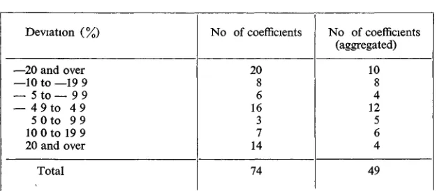
Details of the test shown in Appendix II, and summarised in Table 1 below. The deviations were calculated as follows The difference between the "volume of input" index and the "volume of production" index was expressed as a percentage of the latter, the sign of the deviation being determined by whether the input index was above ( + ) or below (—) its "expected" value, l e the value of the production index
52
TABLE 1
INPUT COEFFICIENTS, DEVIATIONS OF "ACTUAL" FROM "EXPECTED" INDEX OF INPUT
Deviation (%)
—20 and over —10 to —19 9 _ 5 to — 9 9 — 4 9 to 4 9 5 0 to 9 9 10 0 to 19 9 20 and over
Total
No of coefficients
20 8 6 16 3 7 14
74
No of coefficients (aggregated)
10 8 4 12 5 6 4
49
The results of the test do not lend strong support to the notion of stability m input coefficients or, to be more precise, to the assumption of linear proportionality m production functions Of the 74 inputs tested, only 16 (less than one quarter) deviate within plus or minus five per cent, which might be considered "acceptable" limits of variation Even if one is more charitable about the permissible variation, only about one-third vary withm plus or minus ten per cent, and nearly half the coefficients vary by more than twenty per cent It might be objected that the input coefficients of the model will not necessarily vary to the same extent, since inputs tested separately here (detailed in Appendix II) are com-bined in the transactions table and model, so that variability which is the result of substitution may be eliminated or reduced This is best illustrated in the case of the Shirtmakmg industry, for which four inputs listed m the Appendix were tested, the variations ranged from 6-5% to 97-7% If the four inputs are combined, weighted by base-year values, then the index number for the combined input for 1957-58 is 90 7 as compared with the index 90 6 for volume of production This, however, is rather an exceptional case, the result of combining inputs to conform more closely to the mput-output classification of Appendix I is shown m Table 1 The number of inputs has been reduced to 49, but there is no marked improvement in the results
What conclusions may be drawn from the results of the test7 Of the
' 53
individual coefficients, this would not necessarily improve the overall stability of the model6)
Secondly, there is a possibility that the index numbers used are in-accurate, either through errors in statistical sources or m methods of computation This possibility cannot be ruled out, if for no other reason than the fact that an index like the index of volume of production can never be claimed to measure precisely what it is supposed to measure, but it is unlikely that errors of this sort could have had a very significant effect upon the results
There appears little doubt that in many cases the main causes of varia-tion m the coefficients have been input substituvaria-tion and variavaria-tion in the composition of output There is evidence of this in the Census of Produc-tion Reports, and in the details shown in the Appendix, for Distilling, Bacon factories, Gram milling, Sugar, Woollen and Worsted, Shirtmakmg, Clothing, Paper and Oils and Paints Other industries, such as Boots and Shoes, would also have provided examples of input substitution and it been possible to express more inputs in quantum terms Moreover in certain cases it appeared that substitution had occurred between domestic supplies and imports, this does not necessarily affect the input coefficients of the model, if imports and domestic supplies are regarded as homo-geneous and entered in the same rows of the transactions table, but it would affect the results of a projection in terms of the relative supplies of domestic and imported commodities The imposition of additional import levies on many commodities over the period in question was probably responsible for some of the substitution which took place
One conclusion which emerges from the results of the test is that the transactions table is too highly aggregated to allow much reliance to be placed upon the assumption of stability m the input coefficients of the derived model In this context it should be noted that there are more than twice as many separate Census of Production industries as there are industrial sectors in the transactions table. Yet it would require at least double the present number of Census industries, included as separate sectors in the Table, to markedly reduce the effects of variability due to changes in the composition of output This conclusion is perhaps not very surprising, since input-output theory assumes that each sector produces a homegeneous product, and the Irish Table quite obviously does not satisfy this condition In practice, however, it is necessary to compromise between theoretical requirements and practical limitations. The tests described here do not accurately indicate the minimum number of sectors which would be necessary to significantly reduce the effects of aggregation upon the stability of the model, but at a guess it would appear that some 80-100 industrial sectors alone would be required
No attempt has been made here to assess the effects of technical change or non-linear production functions upon the behaviour of the coefficients On the basis of the data collected for the tests, there is some tentative
6 H Thiel—"Linear aggregation in input-output analysis", Econometnca, January
1957 W D Fisher—"Criteria for aggregation in input-output analysis", Review of
Economic Studies, August 1958
54
evidence of both,7 but much more thorough investigation of data is
required before anything definite can be said on this matter This, however, is an important point, since if technical changes or non-linear production functions can be identified one can then ask if they could have been foreseen, if so, allowance could have been made for them in the co-efficients of the model with a consequent improvement in the stability of the model This test was primarily designed to examine the actual behaviour of the coefficients, rather than to analyse the causes under-lying changes in them, so that the data at present available is insufficient for detailed analysis One factor limiting analysis of the published,avail-able sources, however, is the rather broad classification adopted in some of the Census Reports 8
(b) Projection of the Economic Structure
Whilst it is unrealistic to expect input coefficients to remain quite stable over time, one might expect a model employing base-year coefficients to yield reasonably accurate results over a short period The results of the direct tests of coefficients, on the other hand, seem to suggest that the results of a projection (in terms of gross outputs and related aggregates) would not be very reliable If this is the case then the model is of little use for predictive purposes
To this end an alternative test of the stability of the model was tried Using the coefficients derived from the 1956 transactions table, a projec-tion Mas made to 1958, and the answers compared with the "actual" 1958 outputs The very short time period involved was chosen deliberately in order to minimise the effects of technical change upon the coefficients of the model Normally projections of this kind are made "backwards" in time rather than "forwards",9 since the transactions table usually
refers to a very recent year and only one or two subsequent years' data are available But in this case this did not matter as only a short time period was required, and for a variety of reasons 1958 was selected rather than 1954 or 1953
The obvious procedure for carrying out a projection of this kind is to apply a vector of 1958 final demands (revalued at 1956 prices) to the matrix multiplier m (2) and so obtain the vectoV of gross outputs X This "projection" however, was somewhat unusual in that it worked in the opposite direction "Actual" 1958 gross outputs were distributed as intermediate supplies according to the base-year coefficients of the model, leaving a residual figure which, when added to imports, provided an estimate of 1958 final demands This was then compared with "actual"
7 Based on a comparison of time series of inputs and volume of production for the
years 1953-58
8 As a result, inputs and outputs are not specified in sufficient detail in most Census
Reports, and further analysis would require much more detailed statistical information
9 Several such tests have been made in other countries, principally the United
55 .
final demands In short, starting with the 1958 gross outputs, a trans-actions table for 1958 was prepared on the basis of inter-industry relations in 1956
There were several reasons for this treatment First, it was necessary to eliminate errors in the results caused by changes in relative supplies of imports and domestic substitutes, since the test was not concerned with this type of error This of course could have been achieved by changing the import parameters of the model in accordance with "actual" imports in 1958 and recomputing the inverse matrix But it was found very difficult in some cases to distinguish between imports for intermediate use and mports for final demands, applied in the normal way, an error of this type in the final demand vector would have been reflected not only in the gross output estimate of the sector in which it occurred but also, through the inter-industry system, in the output estimates for other sectors By using the "reverse" projection described here this source of error is confined to individual sectors10
Secondly, it was extremely difficult to .construct adequate index numbers of final demands for certain sectors, not only for service-type industries but for certain transportable goods industries such as metals and machinery Once again errors of this sort would have affected the whole system had the normal final demand projection been used, final demand estimates for some sectors were so hazardous that 8 of the 29 sectors in the model were excluded from the test However the inputs of these sectors had to be accounted for in the projection, so that it was necessary to work the projection in the way described The eight sectors involved were simply excluded from the final demand comparison
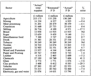
The method employed for the test, therefore, was to calculate total supplies (at 1956 prices) for each of the twenty-one sectors included by adding imports (obtained from the Trade Returns) to "actual" gross outputs (derived from Census of Production data) Total supplies were then distributed as intermediate supplies along the rows of the Table, in the form of a hypothetical transactions table for 1958, and the "remainder" was an estimate of final demands Intermediate supplies were distributed on the basis of the coefficients derived from the 1956 transactions table, assuming linear proportionality between changes in gross outputs and changes in inputs, for each of the twenty-nine sectors The next step was to calculate "actual" final demands from the expenditure flow estimates of the C S O , and the details of imports published in the Trade Returns "Estimated" and "actual" final demands for 1958 were then compared The results are shown in Table 2 below All aggregates are valued at
1956 prices The final figure in each row, " % error", is the difference between estimated and actual final demand, expressed as a percentage of actual final demand, a negative sign indicates that "estimated" demand is below "actual" demand
10 That is, whereas the figure for ''actual" final demands is still subject to this source
. 56
TABLE 2
"ESTIMATED" AND "ACTUAL" FINAL DEMANDS IN 1958 FOR 21 SECTORS
Sector Agriculture Mining Meat processing Creameries Milling Bread Sugar Miscellaneous food Drink Tobacco Textiles Apparel
Wood and Furniture Paper and Printing Leather Chemicals Glass Clay products Vehicles Construction
Electricity, gas and water
"Actual" total supplies £ million 213 175 14 334 31 201 31 660 26 716 13 958 15 659 7 388 31 303 30 249 34 522 32 905 13 937 25 767 6 318 27 189 2 772 5 408 27 503 53 213 21 076 "Estimated" F D £ million 133 250 6 257 28 479 25 733 4 100 13 935 9 459 5 727 28 331 30 249 14 674 32 351 4 164 8 869 2 465 10 740 1 771 0 412 22 187 48 542 14 631 "Actual" F D £ million 130 249 6 925 30 359 25 618 4 971 13 935 9 140 5 684 27 558 30 249 13 863 30 265 5 441 8 743 2 600 7 606 1 876 0 583 22 553 52 460 13 796 / o error 2 3 — 9 4 — 6 1 0 4 —17 5 Nil 3 1 0 7 2 6 Nil 5 9 6 7 —23 4 1 4 — 5 2
41 2 — 5 6 —29 3 — 2 0 — 7 4 6 1
Before considering the results of this test it is necessary to say some-thing about the statistical accuracy of the calculations In some cases these are, unfortunately, subject to such a margin of error that the results must be interpreted with great caution The figures for "actual" gross outputs are, as we have said, based upon the index numbers of volume of production derived from the Census of Industrial Production But it was necessary, for most sectors, to "gross up" these figures to account for output not covered by the Census n For this purpose it was assumed,
for each sector, that the change in volume of production for all establish-ments was proportional to the change in volume of production for all Census establishments. If this is not so there will be errors in the "actual" output estimates, and in some sectors such as Apparel, Wood and Fur-niture and Construction, where there are many small establishments, this could have a significant effect upon the accuracy of the figures
Secondly, as already mentioned it was difficult in several cases to compute reliable indexes of final demands for 1958 The expenditure flow estimates of the C.S O. are themselves subject to revision, sometimes
[image:13.412.57.370.134.394.2]57
substantial revision, in the light of alternative national income estimates12
Moreover the transactions table is highly aggregated and this required in many cases a large regimen for the indexes, some of the products included in the regimen were not specified in quantum terms, and it was necessary to deflate value figures by price indexes whose reliance was questionable It was for this reason, as well as difficulties in separating final from intermediate demands, that certain sectors were excluded from the test, but other sectors included, such as Mining, Textiles, Wood, Paper, Chemicals and Clay Products were subject to the same limitations
The points raised above draw attention to a difficulty which was also apparent in the direct tests of coefficients discussed earlier, and which is of particular relevance to the application of input-output methods in this country That is, the very small scale of industrialisation in Ireland, allied with a considerable multiplicity of product This means that relatively small changes in the composition of output, the entry of a new firm into an industry, marginal changes in technology, etc, can have a significant effect upon the structure of production and hence upon the accuracy of the input-output model Similarly, what might appear relatively minor sources of error in the computation of the index numbers described above can become quite important in relation to small aggre-gates In handling larger aggreaggre-gates the proportionate effect of the errors is often much less
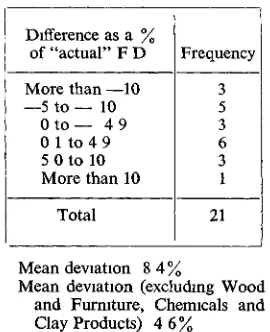
[image:14.419.136.271.413.579.2]The results of the test as shown in Table 2 are also summarised m Table 3 below
TABLE 3
DIFFERENCES IN "ACTUAL" AND "EXPECTED" FINAL DEMANDS 1958
Difference as a % of "actual" F D More than —10 —5 to — 10
0 to — 4 9 0 1 to 4 9 5 0 to 10 More than 10
Total
Frequency 3 5 3 6 3 1
21
Mean deviation 8 4 %
Mean deviation (excluding Wood and Furniture, Chemicals and Clay Products) 4 6%
12 National income calculated from the revenue side is normally lower than the same
58
There are considerable individual variations in the results of the test The mean deviation is 8 4 %, which falls to 4 6 % if the Chemicals, Wood and Furniture and Clay Products sectors are excluded The differences between actual and expected demands in these sectors are so large that it is difficult to believe that technical changes or changes in the composition of output are responsible In fact poor results for Wood and Furniture and Clay Products were expected there are many small (non-Census) establishments, it is difficult to separate accurately final and intermediate supplies, and it was hard to construct suitable quantum indicators for the multifarious products of these industries To some extent similar difficulties were experienced with the Chemicals sector, which manu-factures a very wide range of products, but the error is so large that it seems unlikely to be caused solely by the above factors, and the discrepancy here remains something of a mystery In about half the remaining sectors the "error" is fairly small, I e less than 5 %
To conclude from the "better" results that there is much stability in the input-output model over short time periods would appear to be at variance with the results of the direct tests of coefficients, where the marked variations in many of the coefficients suggested the very reverse of stability in the model Of the two tests, the direct tests of coefficients is to be preferred For one thing, it is more reliable statistically—the scope for inaccuracy in the projection test has already been emphasised More-over, the way in which the projection test w as conducted had a number of disadvantages We have already explained that one reason for under-taking a "reverse" projection was to eliminate errors in the results caused by errors in final demand estimates, since these were irrelevant to a test of the stability of the input coefficients Unfortunately this has a two-edged effect In reality, an unforeseen change in one input coefficient would affect not only one sector but also, through the inter-industry system, the outputs of other sectors as well, and it is desirable that a test of the stability of the model should take this into account But in this test a change in one input coefficient affected only the final demand estimate of the sector which supplied that input, and the iterative (cumulative) effects of the error are eliminated Hence the results as shown above are more flattering to the model than should be the case, since the "good" sector results are immunised from the effects of the poor results in other sectors. In short, the test was conducted in such a way as to eliminate errors in the results which would not have been eliminated had the model been used to project gross outputs in the usual way
59
errors in final demand estimates In this light, and in view of the fact that the test projection was made only over a two-year period, the conclusions to be drawn from the results of both tests are the same That is, that the simple input-output model to which these tests were related is too unstable to be used with any confidence for projections or forecasts of the future economic structure On the basis of the data collected for the tests, the principal reasons for this instability appear to be the high degree of aggregation m the Table, changes in the composition of output, and the relatively small size of the industrial sector in Ireland
It should not be concluded from this that input-output techniques cannot be usefully applied in Ireland The strength of the input-output approach lies in its explicit recognition of the interdependence of sectors of the economy, a factor which must be taken into account in planning or forecasting future economic structure But, largely because of the particular characteristics of the Irish economy, we cannot rely simply upon an .'automatic" input-output model such as that derived from the 1956 transactions table For one thing, a much greater sector classification is required Secondly, the small scale of most industries and the con:
sequently large proportionate effect of changes in the composition of output require a much more empirical approach in constructing the model and in the projection of future gross outputs, rather along the lines of French planning techniques, in which input-output techniques are used in a flexible and continuous process of trial and error, as opposed to reliance on a single formal model based on historical data 13
PART 2: TREATMENT OF IMPORTS IN AN INPUT-OUTPUT MODEL An important methodological problem relevant to input-output applications in Ireland concerns the treatment of imports in the input-output model In this country imports and exports constitute a high proportion of gross national product, so that the assumptions relating imports to other variables contained in the model are very important A variety of methods may be used to incorporate imports into the model, and four of these methods are examined below Although general m outline, the discussion will be centred round the merits and disadvantages of each method for use in an Irish input-output model
Method 1
No distinction is made between competitive and non-competitive imports All imports are included in a single row of the Table, each constituent of which shows the total use by each sector of all imported goods and materials The import row lies outside the main matrix of inter-industry transactions (Quadrant II) and is contained within Quadrant III of the transactions table as part of primary input. It is thus analogous to the row "non-competitive imports" in the transactions table of Appendix I An extension of this method would be the construction of several import rows in Quadrant III, each row showing the use of different
60
groups or classes of imported commodities, but this elaboration would not affect the mathematical model Finished goods imported for direct sale to final buyers are preferably steered directly to the relevant category of final demands (in Quadrant IY), rather than passed through the domestic distributive industry as an input
The principal objection to this nrethod is that it will almost certainly result in unstable input structures The method implicitly assumes that all imports are non-competitive If all imports are non-competitive, at least from the users' point of view, then no problem arises and this method would be adopted, since it is the simplest But if some imports are competitive, than it is doubtful whether the base-year proportions between imports and their domestic substitutes will remain constant, and substitution between the two will occur in response to market forces Hence input coefficients derived from base-year proportions will be liable to instability, with consequent errors in estimates of domestic output levels and the level of imports The larger the proportion of total imports to total supplies, the greater the margin of error In such circum-stances continual amendments (based on current market information) to the original input coefficients would be required, and this would greatly reduce the advantage of simplicity which this method possesses
There are also statistical difficulties in using this method It is necessary to distinguish, m the construction of the transactions table, between inputs of domestic origin and imports Whilst this may not be difficult when all imports are non-competitive, it is so when there are competitive imports, no distinction (between imports and domestic inputs) is made in the Census of Production Reports from which most inputs columns are built up, and imports are not classified by industry of destination in the Trade Returns
The effects of this treatment upon the mathematical model are best seen by examining the inverse of the (I—A) matrix, from the equation
X=(I—A)-lY (2)
Let (I—A)-l=R=[rij] (i, j = l, 2 n)
Each element ry (j = 1, 2, n) in each row l of the inverse matrix R shows requirements of commodity I for the supply of one unit of each
commodity in final demands Y. The elements ry (i = l, 2, n) of each
column j show the amount of each commodity needed to produce one unit of final demand for commodity j Final demands and supplies are of goods of domestic origin only Imports are determined after the model has provided a solution in terms of domestic output levels14 (e g. as linear functions of gross output levels), whilst imports for direct sale to final demands must be separately calculated
Under this method, then, imports are exogenous to the model, the
14 It is possible to construct a row of import requirements r(n_4_ JY., analogous to the
61
model may account for imports only to the extent that changes may be made in the coefficients of the model prior to its application It will be noted that, as a result of this method of construction of the transactions table and the derived model, the variety of imports which constitute an input into any one sector are regarded as functions of the level of output of that sector We return to this point later.
Method 2
The first method makes no analytical distinction between competing and complementary (non-competing) imports. An alternative approach which does make this distinction is to regard competitive imports as purchases by the domestic competing industry, and to distribute total supplies of each "product" along the rows in Quadrants I and II. In this case imports are functions of the level of supplies of goods, rather than functions of the output of those industries which use imports as inputs Consequently, from one angle (the input side) the stability of the model is improved, since the input coefficients of the model are now based upon total purchases of each product, whether imported or domestically produced, and variations in these proportions are irrelevant On the other hand, although the stability of individual coefficients is improved by this treatment, the results of the model will not necessarily be improved since changes may occur in the proportions of domestic supplies and competing imports For instance, if the proportion of imports to domestic supplies of product j rises, and this is not accounted for m the model, then the domestic output of sector j will be overestimated, with consequent effects upon the outputs of other sectors and the level of imports.
Again imports will appear as a row (or rows) in Quadrant III of the transactions table It is convenient to distinguish competitive and non-competitive imports in separate rows, since only the latter are, technically speaking, "inputs" This also has other advantages, as we shall see in a moment A convenient arrangement of the rows in Quadrant III is, therefore, non-competitive imports, other primary input (i e wages, etc ), total domestic output, competitive imports, and total supplies
The elements of the model are now obtained, as follows Xj=gross domestic output in sector j (j = l, 2, n) Mj = competitive imports of product j (j = l, 2, n) mJ=MJ,/XJ
Zj =total supplies of product j (j = 1, 2, n)
The matrix of input coefficients [a^] is first obtained as before, by dividing each column of inputs by gross outputs Xj Then each column of input coefficients is divided by 1 +mj, the resulting matrix is inverted and applied for solutions The ratio l+nij may be changed to allow for variations in the proportions of imports to domestic supplies In mathe-matical form 15
62
Z1=X1+M1
=Xi+miX,
EaijXj=Yi (total supplies—intermediate j = 1 supplies ==final demands)
By substitution
Let aiJ/(l+mJ)=aiJ
Then Zx—I ar,Zj=Yi (i = l, 2, n) J = l
I e Z=(I—A)-l Y (3)
The matrix obtained by dividing each column j of coefficients by 1 +mj may be denoted by A=[aij], which is than used in the solution (3) The solution vector Z for this model is, it will be noticed, in terms of total supplies, from which domestic outputs and imports are easily derived, since Xj=Zj/(l+mj), and Mj=mjXj
It will also be remarked that the vector (mj) of import parameters refers only to competitive imports, whilst non-competitive imports, though also functions of domestic output levels, are separately determined This arrangement, which facilitates any necessary amendments of import parameters, is more satisfactory than including all imports together, the level of competitive imports is, a priori, primarily determined by market forces, whilst the level of non-competitive imports is determined by technical factors
The inverse matrix of this model, which we may denote by R, differs from that of Method 1 in that the element ry (l, j , = l, 2, n) shows total requirements (whether imported or domestically produced) of com-modity I, per unit of final demand of comcom-modity j In Method 1 ry shows domestic requirements only It would perhaps be an advantage if the elements in the inverse matrix of Method 2 were to measure domestic requirements only, rather than total requirements This is easily achieved, if each row j of the inverse matrix R is divided by (1+nij), the resulting matrix, which we may call Ro, shows commodity requirements of domestic origin only, per unit of final demand. Using this matrix Ro with a given vector of final demands Y will provide the same solution for domestic outputs as would occur m using the original matrix R and then dividing each element Zj in the solution vector by (l+nij) It is important to note,
however, that RO^R (the inverse matrix of Method 1)
63
Method 3 i
As we have indicated above, and will further discuss below, there is an important analytical, as well as methodological difference between Methods 1 and 2 Method 3, however, operates upon precisely the same assumptions as Method 2, and will yield the same answers. It is dis-tinguished here in so far as the mathematical treatment is somewhat different, and the Irish transactions table as reproduced in Appendix T is constructed in such a way as to make this method conveneint to use
Total supplies (domestic output+competing imports) are distributed along the rows of the transactions table, as before, but competitive imports are entered as a column of negative outputs in Quadrant I, instead of as inputs into the domestic competing industry Thus whereas the row/column balance between total input and total output is, by Method 2, in terms of total supplies, the balance under Method 3 is in terms of total domestic outputs (vide Appendix I) These, however, are merely alternative ways of presenting the same data, and identical func-tional relationships are postulated by both methods—namely that com-peting imports of any product are a (linear) function of total supplies of that product Non-competitive imports are again entered separately as a row in Quadrant III of the Table
Using the same notation as for Method 2, we have
£ a1 JXJ= Y1 (i = l, 2, . n)
l e ( I + M — A ) X = Y l e X = ( I + M — A ) - l Y ,
where A is the conventional square matrix of input coefficients, M is a diagonal matrix of (competitive) import parameters, and X and Y are the vectors of gross outputs and final demands respectively
Thus method 3 differs from Method 2 in that a diagonal matrix of import parameters is added to the basic (I—A) matrix, whereas under Method 2 the inclusion of imports in the model required an alteration in each coefficient of the (I—A) matrix
The solution is in terms of domestic output levels as opposed to total supplies, although the relations between the relevant aggregates is as before l e Zj=(I+mj)Xj,Mj=mjXj Similarly the inverse matrix differs from the inverse matrix R of Method 2 m that its elements measure commodity requirements of domestic origin only, it is in fact identical with the derived matrix Ro of Method 2, and may be similarly converted
to show total commodity requirements per unit of final demand, by multiplying each row j of the inverse by I + n i j1 6 Solutions in terms of
total supplies, domestic outputs and imports are identical by both methods
Method 4 '
Imports are again distributed with domestic supplies along the rows of the transactions table, and appear m final demands as negative outputs,
16 Alternatively, we may compute an import row analogous to the rows of the inverse
64
as in Table 1, but in the statistical construction of the Table imports and domestic supplies are separately distinguished as inputs There are there-fore three potential entries in each cell of the Table, domestic supply, competing import, and total input (the sum of the first two) We have already referred to this type of table in the Introduction, as an alternative version of the Irish transactions table for 1956
This treatment makes possible a further method of incorporating imports into the model Two matrices of coefficients are derived for the model, one is the familiar [aij] matrix, obtained by dividing each column of (total) inputs by Xj (j = l, 2, n) The second is a matrix of import coefficients M=[mij], obtained by dividing each column of competitive imports by gross outputs Xj =(j = 1, 2 n) The system may be written
-j—2 aijXJ=Y1 (i = l, 2, n) J J
I e (I+M—A)X=Y le X=(I+M—A)-1Y
In the matrix notation the statement of the model is as for Method 3, although in this case the matrix M is to be interpreted as non-diagonal The underlying assumptions of this method, however, are very different from those of Methods 2 and 3
In Methods 2 and 3, total competitive imports of any commodity are built into the model as a function of total domestic supplies of that commodity Thus imports of any one commodity are derived as a certain proportion of competing domestic supplies, I e as a unique function of a single variable By Method 4, total imports of any commodity is a summation, each element of which is derived as a function of the pur-chasing industry's output—thus imports of any commodity is a
multi-valued linear function of the n variables Xi Xn
APPENDIX I
INPUT OUTPUT TABLE FOR 1956 All figures in millions of pounds at Producers Prices
f 1
1 " ""—~^ C o " " " " '1" 1 . --^Industry 1 Industry --| of Origin ^ ^ - ~
1 Agriculture, Forestry, Fishing
2. Mining, Quarrying and Turf
3. Meat Processing
4. Creameries ....
5. Milling, Animal Food
6. Bread, Biscuit and Flour Confectionery
7. Sugar, Cocoa and Choc. Confectionery
8. Miscellaneous Food
9. Drink
10. Tobacco
11. Textiles
12. Apparel
> 13. Wood and Furniture
k
; 14. Paper and Printing ' IS. Leather and
Manufactures
16. Chemicals
17. Glass. Pottery
18. Structural Clay and Cement
19 Metal and Shoe Forging
20. Machinery 21. Vehicles 22. Miscellaneous Manufactures 23. Construction 1 4.743 0.818 0.014 0.036 13.993 0.733 0.561 0.314 1.379 0.188 7.957 2.109 0.578 0.700 0.275 0.100
24 Electricity. Gas, Water 0.420
25. Transport and Trade
26. Communications
> 27. Finance
Jfc. -28 Ownership of
%•" Dwellings
KL —
•* 29. Public Administration ^ ^ and Defence
n 30. Education, Health and • t Veterinary Services
f
F 31. Other Professions
6.781 0.045 2.026
1.240
* 32. Hotels and Restaurants
33. Amusements, Recreation
34. Laundries, Hairdressing
<* 35. Domestic Servants
36. Other Personal Services
37. Sales by Final Buyers
1 Total Inter-Industry Input
1 Non-competitive Imports | c.i.f.
45.010
2.038
1 Indirect taxes (including 1 rates) less capital grants, 1 subsidies and transfers 8.284
1 Wages, Salaries, Pensions, H Employers'
Contribu-H tions to S. 1. 20.083
| and Rent 105.500
H Total Primary Input 135.905
H Total Input 180.915 2 0.024 0.027 0.028 0.044 0.051 0.177 0.091 0.275 0.206 0.018 0.154 0.018 1.113 0.945
- 0 . 0 7 8
3.758 3 2I.55S 0.048 4 20.640 0.141 S 17.098 0.047 6 0.101 0.024 7 4.1 II 0.229
1.307 0.017 0.140 0.255
0.010 0.044 0.156 0.004 0.239 0.179 0.040 0.097 1.412 0.060 0.110 0.029 25.290 0.734 0.110 2.443 1.044 0.952 5.669 4.239 6.782 29.529 4.579 1.874 0.008 0.004 0.066 0.422 0.095 0.107 0.119 0.440 0.076 0.130 0.022 28.740 0.949 -2.575 1.550 0.718 2.910 0.004 0.419 0.392 0.116 0.096 0.236 1.919 0.051 0.283 0.048 23.759 3.330 -6.480 2.104 1.489 0.148 4.910 0.569 0.739 0.021 1.796
0.970 | 0.204
0.182 0.235 0.038 0.055 0.096 0.278 0.570 0.023 0.09 8 0.027 8.579 0.997 0.347 3.698 1.169 0.001 0.942 0.019 0.050 8 0.946 0.019 0.005 0.085 0.571 0.257 0.171 1.051 0.223 0.427 0.024 0.031
0.082 | 0.036
0.610 0.026 0.139 0.012 0.361 0.012 0.064 0.006 9 3.302 0.244 10 0.009 0.003 | 0.306 0.085 , 2.110 0.211 0.381 0.029 0.127 0.184 0.116 0.008 0.094 0.407 0.026 0.087 0.036 I I 1 I 8.981 i 1.757 0.174 X270 0.422 4.289 0.446 0.102 0.916 0.547 7.753 1.313 14.034 4.234 4.310
0.642 0.443 6.211 4.623 2.011 23.891
29.382 24.202 14.790
H NOTE: This Input-Output table his not been amended t o Cake account of
13.604 t 6.300 31.644
my changes in the National
-i . . . i-i
0.624 0.026 0.019 0.135 0.025 0.046 0.005 0.895 4.395 23.285 1.221 1.239 30.140 31.035 Account I I 3.207 0.066 0.004 5.975 0.156 0.225 0.041 0.120 0.095 0.202 0.682 0.033 0.187 0.027 0.459 11.479 2.522 0.093 3.873 2.108 8.596 20.075 13 0.759 0.005 _ -0.392 4.160 0.060 0.010 0.169 0X129 0.258 0.046 0.060 0.092 0.288 0.029 0.162 0.019 14 0.115 0.101 15 0.S83 0.020 0.739 0.024 0.001 0.026 6.730 0.011 0.123 0.129 0.127 0.008 0.307 0.734 0.001 0.037 0.017 0.031 1.002 0.066 0.033 0.485 0.089 0.009 0.166 0.026 1 • -0.047 6.585 0.14! 0.118 3.386 1,028 0.220 8.913 0.707 0.267 5.823 2.154
I 4.673 8.951
»11.258 Aggregates 17.864 0.046 0.004 3.097 0.498 0.029 0.777 0.417 1.721 4.818 16 0.323 17 0.022 0.150 0.154 | 0.116 0.022 0.008 0.006 0.032 0.069 0.770 4.407 0.011 0.413 0.043 0.090 0.551 0.031 0.096 IS 0.001 0.899 0.029 0.025 0.121 0.080 0.001 0.075 0.139 0.021 0.087 0.020 0.026 7.162 2.359 0.163 1.941 0.903 5.366 12.528 0.776 0.277 0.059 0.943 0.062 1.341 2.117 0.004 0.036 O.43S 0.016 0.432 0.071 0.265 0.674 0.014 0.060 0.018 2.725 0.913 0.084 1.379 1.096 3.472 6.397 19 0.001 0.112 0.001 0.083 0.108 0.098 0.036 4.021 0.233 0.645 0.028 0.148 0.016
(Competitive imports distributed as part of
20 0.006 0.167 0.080 0.073 0.036 0.920 1.171 0.110 0.346 0.020 0.062 0.012 0.457 5.987 1.120 0.084 3.152 1.282 0.008 3.011 1.310 0.087 1.676 0.712 5.638 3.785 11.625 6.796 21 0.017 0.029 22 0.014 0.041 0.023 0.138 0.256 0.080 0.013 0.145 0.064 0.438 0.363 1.341 0.496 0.134 0.555 0.027 0.061 0.017 4.197 6.002 1.068 4.345 0.428 .044 0.587 0.250 0.144 0.041 0.012 0.149 0.303 0.112 0.194 0.016 0.060 0.017 1.984 1.929 0.097 1.944 0.841 23 0.006 1.146 0.004 4.181 0.209 0.831 0.217 5.996 5.395 1.706 0.048 0.455 1.828 0.474 5.652 0.087 0.849 0.144 29.228 2.273 0.662 32.201 4.834
11.843 I 4.811 39.970
16.040 6.795 69.198 24 0.001 1.156 0.024 0.227 25 0.839 2.023 0.020 0.014 0.048 0.589 0.130 3.345 0.302 0.027 0.717 1.917 0.157 0.093 1.202 0.073 0.147 0.042 5.783 4.193 0.771 6.120 4.344 15.428 21.211 0.266 0.103 0.596 3.055 0.978 1.000 0.672 1.742 1.300 1.612 0.500 0.124 20.258 t7.235 8.467 43.420 27.700 26 each 27 1 0.060 0.010 0.124 0.068 0.044 0.746 0.110 0.491 t0.382 2.035 0.078 0.157 5.366 2.282 86.822 7.883 107.080 9.918 row) 28 29 9.400 10.504 1 19.904 19.904 —4.255 17.400
30 31 32 33
1
i
34 35 36
0.123 0.004 0.809 | 30.670 20.205 5.810 0.065 1 0.077 0.004 , 0.003 0.060 0.200 0.030 0.250 , 0.150 0.300 O.3S3 0.150 0.326 +0.996 0.105 0.044 0.046 0.160 0.078 0.250 ' 0.04S , 0.250 ' 0.130
0.050 7.101 2.280 2.317 0.217 0.247 2.800 1.948
13.145 30.670 26.085 i 9.351 5.212
13.145 30.670 26.085 9.381 7.529
bsequent to the original compilation of the table.
0.050 0.025 0.005 0.141 2.225 0.143 2.963 1.990 1.503 6.599 8.824 0.737 0.216 0.038 1.611 1 I.I0S 7.850 1.300 0.130
2.970 7.850 1.430
3.707 7.8S0 1.430 3T Total Inter-mediate Output 78.221 8.599 2.646 5.517 38 39 House- vcm-holds nent Excl. irrent Touristl^et 40 Govern-' ment Capital 41 Other Capital
67.96! 0.587 0.723
5.7010.100 0.936
42 43 44 Stock Exports Total Changes Final Output 45 46 Total Less Output Com-petitive Imports
—1.433 J49.30I 117.145 , 195.366 , t—14.451
-0.320 0.602 ' 7.018
15.79:0.060 0.112 JI2.I5I
16.90! 0.035
22.082 3.98! 0.030 |
0.021 14.265 0.030
5.871 8.5270.010
1.694 l| 5.302
3.075 21.192 20.016 0.571 11.150 17.020 3.911 15.606 1.053 6.491 15.991 6.375 5.212 29.189 6.839 1.207 29.1420.272 0.023
3.8900.050 0.047 1.045
5.1170.500
0.388 0.007
6.148 !
0.726 0.457
0.050
4.661 0.006 1664 3.8230.037 ! 2.349 5.4420.024 0.019 13.740
3.828 6.2633.045 0.189 5.088 ;| 3.4221170 22.053 27.471
6.670 1 8.2273.900 0.091 5.209
30.360 S5.799D.I00 3 359 3.030 7.553 1.240 1.256 0.124 0.141 1.191 5.6311500 7.9253.300 0.126 13.145 3.670 II.7IS3.I30 8.125 5.102 5.700 3.J66 7.850 1.430 —4.610,
291.603 II 3M.J44
49.450 48.722 251.224 211.842 561.238 852341 —1.300
1.550 23.065 56.356
13.630 >.5O0 29.1961250 I* LlOO 15.566.850 | 378.7781.400 0.149 47 Total i Domestic Output 180.915 Consuming ^^^^~^~ Industry ^--Industry . ' of Origin
1. Agriculture. Forestry. Fishing
2. Mining. Quarrying and 15.617 -8.835 6.782 Turf
28.115 , 30.761 t 1 232
0.355 J7.737 25.032
+0.158
—0.036 0.350 {1.642 —1.526 i 12.531
4.527
15.901 9.542 - 0 . 0 7 6 0.634 | 5.860 '0.588 J 10.371 32.151 ^0.329 J2.566 32.034 -0.422 J4.926 13.394 -0.206
- 0 . 1 4 0 - 0 . 2 5 0 J-0.095 1-0.120 ~ 0.031 £5.098 0.372 13.751 1.964 0.590 $0,716 0.009 0.661 + 0.595 X 1.076
- 0 . 1 3 9 | 0.840 —0.041 J0.342 - 0 . 0 2 5 J 1.476 - 0 . 0 0 6 |
34.741 S.264 9.618 2.454 6.858 1.930 0.720 8.002 6.910 19.526 7.948 64.110 - 0 . 5 5 2 1 14.979 - 0.688 J20.099 80.045 to. 139 7.270 ;4.000 12.351 1 13.145 30.670 24.845 8.125 J4.5OO 23.000 9.602 8.700 3.566 | 7.850 1.430 - 1 . 7 3 0
30.549 t - I . I 67
26.609 ! 1407
15.922 15.413 7.5S4 35.226 t—1.132 t-1.809 —1.254
29.529 3. Meat Processing
29.382 4. Creameries
24.202
14.790
13.604
6.300
5. Milling, Animal Food
6. Bread, Biscuit and Flour Confectionery
7. Sugar. Cocoa and Choc. Confectionery
8. Miscellaneous Food
* 3.582 31.644 9- Drink
32.084 + 1.049 31.035 1 10. Tobacco 33.410 13 335 20.075
35.312 16.414 26.638 6.365
1 1. Textiles
+ 2899 ! 32.413 . 12. Apparel
—5.156 11.258 i 13. Wood and Furniture
—8.774 I 17.864 ' 14. Paper and Printing
1 547 4.818 IS. Leather and Manufactures
22.464 9936 12.528 16. Chemicals 2.983 —0.866 2.117 17. Glass. Pottery 7.211 23.993 13.285 24.738 11.776 69.198 21.649 110.405 10.300 19.904 13.145 30.670 26.085 9.381 9.602 8.824
18. Structural Clay and —0.814 6.397 ! Cement
12368 H.625 19. M « i l 4 Shoe Forging
_ * . « 9 6.796 1 20. Machinery
-8.698 16.040 21. Vehicles
22. Miscellaneous 4.981 6.795 Manufactures
69.198 23. Construction
—0.438 21.211 24. Electricity, Gas, Water
+-3.325
+-O.382 , 9-918 26. Communications
19.904 | 27. Finance
13.145
28. Ownership of Dwellings
29. Public Administration 30.670 and Defence
30. Education. Health and 26.085 Veterinary Services
9.381 31. Other Professions
t 2 073 7.529 32. Hotels and Restaurants
33. Amusements, 8.824 Recreation
3.707 3.707 34. Laundries. Hairdressing
7.850 7.850 35. Domestic Servants
1.430
36. Other Personal 1.430 Services
• 6 . 4 4 9 , -1.191 37. Sales by Final Buyers ^-0.962 147.884 680.237 : 971.840 -118.999 852.841 Total Inter-Industry Input
9.750 -0.688 1.535 24.876 74.326 ^ J Non-competitive lm p o r Q
Indirect taxes (including
- " « » ' 0 * 0 1.151 38.396 .0.326 10.326 " £ * « a n d ^ ' f n s S
1.
1
4.952 4.952 2S6.I76 -0.281—6.900 41.032 36.232 248.074 —17.050
0.149 0.801 - 6 . 9 3 8 46.368 27.664 588.902 -17.331 23.214 57.IS7
»r partly inv isble impor
—7.900 194.252 707.901 i
.560.742
t W h o l l y o r partly invisible e x p o r t .
Wages. Salaries. Pensions, • Employers' Contribu-255.895 ' tions to S.I.
i n «-.. P r°f l Is (incl. depreciation) 231.024 and Rent
571.571 Total Primary Input
65
for structural analysis of the economy, and may also enable us to make more accurate changes in import parameters
The question arises as to the best method to use, particularly with respect to Irish conditions Basically this involves a choice between Methods 1 or 4 and Methods 2 or 3 Methods 2 and 3 differ only in the formal mathematical treatment and provide the same solutions in all circumstances, it does not matter which is used For convenience in the ensuing discussion we shall assume that Method 3 is adopted It is also convenient to exclude Method 1, since this is merely a less detailed version of Method 4, so that the choice is reduced to one of two methods
In the light of our description of the different methods, it would appear that a model using Method 3 would be more stable than a model using Method 4, and that the former should therefore be adopted Under certain conditions, however, Method 4 will provide solutions which are conceptually and statistically better than those of Method 3 These con-ditions are related to (I) the homogeneity of imports and competing domestic supplies, and (n) the relative proportions in which imports and domestic supplies are distributed along the rows of the transactions table If competitive imports and domestic supplies were quite homogeneous from the users' point of view, it would be difficult to justify the calculation of the import matrix M of Method 4, since the coefficients would be subject to more or less arbitrary variation (this difficulty would also apply to the import parameters of Method 3, but to a lesser extent)
Secondly, if domestic supplies and competitive imports were dis-tributed along the rows of the transactions table in equal or similar proportions, then Method 4 would always yield the same or very similar results as Method 3, and would therefore be largely redundant—Methods 2 or 3 being simpler
There are reasonable grounds for supposing that, in Ireland, a fairly high proportion of "competitive" imports are not strictly speaking com-petitive at all, and that their classification as "comcom-petitive" rests upon the fact that they are classified in the same industrial group as certain domestic products, e g "machinery", "metals", etc In this case it may be argued that domestic supplies and competitive imports will be required in fairly stable proportions as inputs, and that the overall level of imports of any commodity is determined by the level and structure of domestic outputs Allied to this, the variation in proportions in which competitive imports and domestic supplies are distributed along the rows of the Irish transactions table means that if there is a marked change in the structure of outputs then Method 4 will provide different, and theoretically better, results from those based upon the assumptions of Method 3
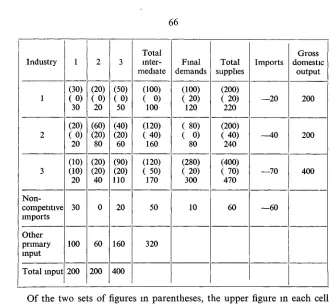
66 Industry 1 2 3 Non-competitive imports Other primary input Total input 1 (30) ( 0 ) 30
(20) ( 0 ) 20 (10) (10) 20 30 100 200 2 (20) ( 0 ) 20 (60) (20) 80 (20) (20) 40 0 60 200 3 (50) ( 0 ) 50 (40) (20) 60 (90) (20) 110 20 160 400 Total inter-mediate (100) ( 0) 100 (120) ( 40) 160 (120) ( 50) 170 50 320 Final demands (100) ( 20) 120 ( 80) ( 0) 80 (280) ( 20) 300 10 Total supplies (200) ( 20) 220 (200) (40) 240 (400) (70) 470 60 Imports —20 —40 —70 —60 Gross domestic output 200 200 400
Of the two sets of figures in parentheses, the upper figure in each cell represents input of domestic origin, while the lower (middle) figure shows the input of competitive imports The third figure shows total input. Linear input coefficients were derived from this transactions table (certain rearrangements were made depending on the method used) and a new set of final demands of 100, 100 and 400 respectively were postulated For Method 4, final demands for imports and domestic products were assumed to move proportionately The results of the two models, l e the solution vectors of domestic outputs, were as follows
Industry 1 2 3 Method 3 200 248 522 Method 4 205 247 527
[image:24.415.39.370.53.357.2]67
which competitive imports were included fell, whilst intermediate de-mands, relying solely on domestic supplies, rose, thus the proportion of imports in total supplies fell
The strength or weakness of the approach in Method 4 depends upon the extent to which -"competitive" imports and domestic supplies are regarded as perfect substitutes If, as we have suggested, there are in many cases distinct differences between "competitive" imports and domestic supplies, the level of imports is determined by primarily technical factors and there is a good case for adopting Method 4, despite the statistical difficulties involved
The assumptions involved in Method 3 imply a marketing rather than a technical relation between imports and domestic supplies, since under this method changes in the composition of demand for any product have no effect upon the import ratio Both the "marketing" and the "technical" factors are presumably present, but without further detailed study of mter-mdustry relations it is not possible to determine the quantitative importance of each factor If the "marketing" factor were considered predominant, this would imply that competitive imports were homo-geneous with domestic products, I e were close substitutes, and imports would be "explained" by marketing factors In such circumstances Method 4 would be of doubtful value, since the coefficients of the import matrix would be highly unstable, under the influence of fluctuations in market forces There would indeed be no logical foundation for Method 4, and Method 3 would be preferred
Moreover, Method 3 (or 2) is theoretically the best method to aim at If the "technical" factor is found to be important, this implies that many imports which have been classed as "competitive" should in fact be included with non-competitive imports The advantages of detail need not be lost, since we can have as many rows of non-competitive imports in Quadrant III as are desired We can in fact employ a method which is a combination of Methods 3 and 4, and possesses the advantages of both
The preceding discussion has been concerned with the basic assumptions which are relevant to the treatment of imports m an input-output model, and additional problems which may be examined have been ignored, e g the use of marginal or average import coefficients It is also desirable in an Irish model that imports of goods for final demands be estimated separately, rather than be derived as simple linear functions of total supplies Thus the principal aim of the model would be to evaluate the level of imports of semi-processed goods and materials
68
APPENDIX II
INPUT-OUTPUT SECTORS AND CORRESPONDING CENSUS OF INDUSTRIAL PRODUCTION INDUSTRIES INDIVIDUAL INPUTS
TESTED AND DEVIATIONS
Sector
2 Mining, quarrying and Turf
3 Meat processing
4 Creameries
5 Gram milling and animal food
6 Bread, biscuit and flour confectionary
7 Sugar, cocoa and chocolate confec-tionery
8 Miscellaneous food
9 Drink
10 Tobacco
Census industries Coal mining, stone, slate, sand and gravel, misc mining and quarrying, turf and bog development Bacon factories, slaughtering etc of meat other than by bacon factories Creamery butter, condensed milk, cheese, etc
Grain milling and animal food
Bread, biscuit and flour confectionary
Manufacture and refining of sugar, cocoa, chocolate
Canning of fruit and preserves, jams, jellies, canning and preserving fish, butter blending, margarine and fats, miscell food preparations Disti.lmg
Malting Brewing
Aerated and mineral waters.
Tobacco.
Inputs tested
None
Bacon pigs Pork pigs Cattle and beef
Whole milk Cream Sugar Raw cocoa Wheat Barley Maize Offals Wheaten flour Sugar Margarine oils Beet
Refined sugar Butter cocoa Raw cocoa Fruit Vegetables Sugar Butter Fats and oils
Barley Other grains Malt Molasses Barley Barley Malt
Raw tobacco
Deviation(%)
—
32 0 —58 9 —35 5
11 1 13 7 —27 4 —67 9 4 7 117 7 —77 6 35 7
3 4 — 7 5
2 0
Nil —35 7 —66 9 ^20 8 19 6 32 5 10 7 36 0 4 0
19 7 —31 3 —32 0 23 5 7 0 7 9 3 3