DETECTION ENVIRONMENT FORMATION METHOD FOR ANOMALY DETECTION SYSTEMS

4270

GLOBAL STABILITY OF SEIR MODEL WITH LYAPUNOV

FUNCTION METHOD WITHIN COMPLEX NETWORK

DOUNIA BENTALEB1_{,SAIDA AMINE}2_{, ZAKARIA KHATAR}3

1,2_{Laboratory Applied Mathematics, FST Mohammedia, University Hassan II of Casablanca, Mohammedia,}

Morocco

3_{LaboratorySSDIA, ENSET Mohammedia, University Hassan II of Casablanca, Mohammedia, Morocco}

E-mail: [email protected] _{, [email protected]}2_{, [email protected]}3

ABSTRACT

In this paper we performed a mathematical study of an SEIR epidemic model on dynamical network. We propose a mathematical SEIR model that consider Watts-Strogatz type complex network that involve contact among individuals. The stability conditions are obtained by using the Lyapunov function, and interpreted using a new threshold noted Ks. In order to show the effect of the network structure on the disease transmission and its asymptotic behavior. Using an algorithm programmed in R, a numerical simulation is presented to illustrate the influence of the small world network properties on the spreading of the disease in our model. This simulation can be used to determine the statute of different diseases in a region using data in this region and the corresponding parameters of the infectious diseases.

Keywords: SEIR Epidemic Model, Complex Network, Lyapunov Function, Global Stability, Infectious Diseases.

1. INTRODUCTION

Mathematical epidemiology has a long history in the study of infectious diseases. Starting with daniel bernoulli in 1760 when he developed a model for the spread of smallpoxand and established a new analysis of smallpox mortality and the benefits inoculation to prevent it [1]. Then continuing with Ross, Hamer, Mc kendrick and Kermack who established the foundations of the epidemiology approach based on compartmental models, between 1900 and 1935 [4].

In 1911, Ross gived the first compartmental model using differential equations to describe the dynamics of malaria [15], where he has divided the population into two compartments S the susceptible and R the recovered individuals, and used the concept of threshold elementarily, without naming it. This notion was later established by Kermack and Mc Kendrick in 1927 in their famous threshold theorem [9]. This threshold is represented by the basic reproduction number R0, which is interpreted as the average number of new cases generated by an infectious subject in a susceptible population.

The standard representation of a compartmental model is a graph . The vertices represent the compartments and the arcs are weighted by the fractional transfer functions. Nodes are often represented by rectangles, circles, or dots.

Several models exist in the literature modeling the various statues of the disease during the infection. The population may be divided according to the nature of the disease into several compartments representing the different steps of infection, for example SI (susceptible, infected), SIR (susceptible, infected, removed), SEIR (susceptible, exposed, infected, removed), etc. The simplest epidemic models suppose that the population is homogeneous. So that, each individual has the same probability of contact with any other individual in the graph . This hypothesis is not realistic.

Lately, models gained an increasing level of complexity[24,25,26,27,28]. Many authors were interested in stochastic models [8,16,7] and other in the effect of the network structure of contacts on the disease transmission [20,12,2,22]. In order to be more realistic and predictive.

Including the effect of networks in classical models, helps to study the impact of spatial structure and serve to better understand the structure of social contacts. In networks the members of population are modeled

4271

(2)

(1) p=1 the lattice is poorly clustered [13]. The small world (SW) network is between them neither highly clustered like regular nor poorly clustered like random network, and in this network infectious diseases spread more easily [23].

The aim of this article is to study the spreading of infectious disease in the small-world network, in order to better understand the structure of social contact networks and their role in epidemiology. Many authors have been interested in SW networks : Samaki and Kaski have studied the SIR model in SW [19]; Han studied the SI model disease spreading with epidemic alert on SW [5]; Liu and Xiao studied the local stability of SEIR in SW [12]; Wang Cao Alsaedi and Ahmad considering infection across the edge on random networks [22].

In this work, we study the stability of the SEIR model in SW. We prove the global stability using a Lyapunov function. We give a new expression of the threshold which involves the degree of distribution of the SW. Which leads us to propose an equivalent threshold that will show the influence of social contact in the disease spreading on small world.

2. MODEL FORMULATION

The total population at time t, denoted by N(t), is subdivided into four disjoint classes S(t), E(t), I(t) and R(t). With S(t) denoting the number of susceptible individuals at time t, E (t) the number exposed of individuals, I(t)the number of infective individuals, and R(t) the number of recovered individuals, the model takes the form,

With :

µ

: Birth and death rate proportional to total population N,

α

: Rate of transmission of the disease,

β

: Rate of exposed individuals who become infectious,

γ

: Recovery rate.

In the following we note: a = µ+β and b = µ+γ. From the system (1) we have :

Where :

s(t)=S(t)/N, e(t)=E(t)/N, i(t)=I(t)/N and

r(t)=R(t)/N indicating the density of S(t), E(t), I(t)

and R(t) respectively.

The term αN s(t) implies that all the infectious can contact all the susceptibles, in other words the graph modeling the population is completely connected, In the Small world complex network [23], of which each node has <k> links on the average, the assumption of complete connection seems unreasonable, hence the interest of implementing the small world network in the previous model.

2.1 Small world complex network

A complex network is a set of nodes and links linking them to each other. Different types of networks are defined according to the nature of the nodes and the links fig (b), (c) and (d). In social networks, nodes, also called network actors, can represent individuals, organizations, or groups of individuals and the links represent the interactions or social relations between the actors of the network: kinship, collaboration between businesses, sexual relations.

The small world complex network is between the regular network and the random network.

The small world network is closer to reality. The nodes in this network are linking between each others with a probability p with (0 < p < 1) fig (e). It is a network within which the propagation of information is faster, while retaining certain properties of conventional networks. Moreover, between any pair of vertices, there is a very short path that can be found easily. In this paper, we are interested in this model. One of the parameters characterizing the network is < k > the average degree of distribution and which represents the average number of neighbors an individual can have in the network.

4272 (3) network are random. So in the equations of evolutions they introduce the degree of distribution of the law between nodes noted by < k > . This modeling is more realistic because the connection between nodes is not sure . < k > is the average of this distribution law.

(a)

SEI- small world model

Hence the interest of replacing the term αN s(t)

with α<k>s(t), where <k> is the average degree of distibution [13], that represent the average number of neighbors that an individual can have in the population [14,10]:

Further, unlike in the aforementioned modeling studies, detailed rigorous mathematical analysis of the model (3) represented in figure (a) will be provided.

(b)

Regular model

(c)

Small world model

(d)

Random model

4273

(3)

2.2 Basic Properties

Our model monitors human populations, so all its associated parameters must be nonnegative. Further, the following nonnegative result holds.

Theorem 2.1.

Let the initial data for the model be positive

s(0) ≥ 0, e(0) ≥ 0, i(0) ≥ 0 and r(0) ≥ 0, then the variables of the model s(t), e(t), i(t) and r(t) will remain positive for all solutions of system (3) for all t>0.

Proof. Let be

T=sup{τ ≥ 0 |∀ 0 ≤ t ≤ τ such that s(t) ≥ 0, e(t) ≥ 0, i(t) ≥ 0, r(t) ≥ 0}. Let’s prove that T=+∞.

Suppose that 0< T < +∞ then by the continuity of solutions we will have : s(T)=0 or i(T)=0 or e(T)=0

or r(T)=0. If s(T)=0 then :

s(T)=0=>𝒅𝒔(𝑻)

𝒅𝒕

=

𝐥𝐢𝐦𝒕→𝑻 𝒔(𝑻) 𝒔(𝒕)

𝑻 𝒕

=

𝒕→𝑻𝐥𝐢𝐦 𝒔(𝒕) 𝑻 𝒕 ≤ 0

But from the first equation of the system (3) we have 𝒅𝒔(𝑻)

𝒅𝒕 = µ > 0. Similar proof for e(t), i(t) and

r(t). So T could not be finite, hence, all solutions of model (3) remain positive for all time t > 0 as required. This concludes the proof.

2.3 The invariant set

Since the population is constant so:

s + e + i + r =1 i.e. r = 1-s-e-i

And solutions are positive as shown in the theorem 2.1, so we are interest in working only in the positive orthant.

Proposition 2.2.

The closet set G is positively invariant, such that:

G={(s,e,i,r)

∈

𝑹

𝟑

such that s+e+i+r ≤ 1}

Proof.

Let be H: R R defined as:

H(s , e , i) = s + e + i – 1

So for all,

(s,e,i) ∈ H-1_{(0)={(s,e,i) ∈ 𝐑}𝟑 _{∶ 𝐇(𝐬, 𝐞, 𝐢) = 𝟎},}

we have:

<𝛁H(s,e,i),(s’,e’,i’)>=<(1,1,1),(_𝐝𝐭𝐝s, _𝐝𝐭𝐝e, _𝐝𝐭𝐝i)>=-γi≤0.

Therefore, according to barrier's theorem [17, 6], G is a positive invariant set for the system (3).

3. STABILITY OF THE DISEASE FREE EQUILIBRIUM

The system has an unique Disease Free Equilibrium (DFE) given by:

E

0

=(s

*

,e

*

,i

*

)=(1,0,0)

(4)

3.1 Local stability of Disease Free Equilibirum

In this section we will study the local stability of Disease Free Equilibrium.

Theorem 3.1.

The Disease Free Equilibrium E0 of the model (3),

given by (4), is locally asymptotically stable (LAS) if R0< 1.

Proof.

The local stability of the DFE is studied using the Poincaré-Lyapunov theorem [3], we first start by calculating the R0 using the next generation matrix FV-1 _[21]:

R

0

=ρ(FV

-1

)

Where F is the nonnegative matrix of the new infection terms, and V is the M-matrix of the transition terms associated with the model (3), so:

Hence the basic reproduction number is given by:

R

0

=

α

<k>

𝜷

𝒂𝒃

(5)

4274

(9) The jacobian matrix of the system is given by:

The jacobian matrix of the system in the DFE is given by:

The characteristic equation:

| J(E

0

)-λI |=0

i.e.

(a+λ)(b+λ)-βα<k>=0

It is clear that this characteristic equation has one positive real root if R0>1, and two negative real roots or two complex conjugate real roots with negative real parts if R0<1. This concludes the proof.

3.2 Global stability of Disease Free Equilibirum

To investigate the global stability of the DFE we use the Lyapunov method.

If a V function is globally positive defined, Radially unbounded and its temporal derivative is globally negative,

𝑽̇

(x) < 0 for all x

≠

x

0

Then the equilibrium x0 is globally stable.

In our model the proposed Lyapunov function is:

V(s,e,i)=

𝟏

𝒂

(s-s

*

_-s

*

_ln

₍

𝒔 𝒔∗

)

)+

𝟏

𝒂

e+

𝟏 𝜷

i

Theorem 3.2.

Assume R0<1, Then the Disease-free equilibrium of the model (3), given by (4), is Globally Asymptotically Stable on G.

Proof.

Consider the following candidate for a Lyapunov function on G:

V(s,e,i)=

𝟏 𝒂

(s-s

*

_-s

*

_ln

₍

𝒔 𝒔∗

)

)+

𝟏

𝒂

e+

𝟏

𝜷

i

(7)

At DFE, E0, it is clear that V(E0)=0. To establish that V > 0 for all (s,e,i) ≠ (1,0,0), it is sufficient to notice that:

𝟏 𝒂

(s-s

*

_-s

*

_ln

₍

𝒔

𝒔∗

)

)> 0 i.e.

𝒔∗

𝒂

(

𝒔 𝒔∗

-1-ln

(

𝒔 𝒔∗

)

) > 0

Since the function f(x)= x-1-lnx reaches its global minimum in x=1 and f(1)=0 then f(x)>0 for all

x ≠1 hence:

V (s,e,i)> 0 for all (s,e,i) ≠ (1,0,0)

Furthermore, it is also clear that V is Radially unbounded:

V(s,e,i) ∞ when ||x|| ∞

The temporal derivative of V is given by:

𝑽̇(s,e,i)= 𝟏

𝒂(1- 𝒔∗

𝒔) 𝒅 𝒅𝒕 s+

𝟏 𝒂

𝒅 𝒅𝒕 e+

𝟏 𝜷

𝒅

𝒅𝒕 i (8)

Let's prove that the temporal derivative of V is strictly negative for all (s,e,i) ∈ G and

(s,e,i) ≠(1,0,0).

Hence, if R0 < 1 we have 𝑽̇ ≤0 and the set

L={(s,e,i) ∈ G such that 𝑽(̇ _{s,e,i)=0} is reduced to}

E0.

Therefore, according to the Lyapunov theorem, the Disease Free Equilibrium is Globally Asymptotically Stable on G when R0 <1.

4. STABILITY OF THE ENDEMIC EQUILIBRIUM

In this section we are going to explore the local and the global stability of the endemic equilibrium. Since solutions are positive as shown in the theorem 2.1, the following result holds.

Proposition 4.1.

If R0>1

,

then the system (3) has a unique endemic

equilibrium.

4275

4.1 Local stability of the Endemic Equilibrium

In this section we investigate the local stability of the endemic equilibrium.

Theorem 4.2.

The Endemic Equilibrium E1 of the model (3),

given by (9), is locally asymptotically stable (LAS) if R0 > 1.

Proof.

As done previously in the proof of the theorem 3.1, we start by calculating the jacobian matrix of the system in the EE.

The characteristic polynomial:

P(λ)=λ

3

_+λ

2

_(µR

0

+a+b)+λµR

0

(a+b)+µab(R

0

-1)

Using the Routh-Hurwitz Criteria [11], to prove the negativity of the eigenvalues, it is sufficient to verify that:

1)- (µR0+a+b)>0,

2)- µab(R0-1)>0,

3)- (µR0+a+b)µR0(a+b)> µab(R0-1).

The first condition is already verified, the second one is verified if R0>1, and for the third inequality

we have:

(µR0+a+b)R0(a+b)-ab(R0-1)=R0(a2+b2+ab+µ)+ab

Which is positive, hence, if R0>1 all the roots of the

characteristic polynomial are negative or have negative real parts. This concludes the proof.

4.2 Global stability of the Endemic Equilibrium

Lemma 4.3.

Let x1, . . . ,xn be n positive numbers.

Then their arithmetic mean is greater than or equal to their geometric mean

:

Theorem 4.4.

Assume R0 > 1. Then the Endemic Equilibrium of

the model (3), given by (9), is Globally Asymptotically Stable.

Proof.

Consider the following candidate for a Lyapunov function on G.

V(s,e,i)=s-s**_-s**_ln(

∗∗+e+e

**_-e**_ln(

∗∗)+ µ

(i-i**_-i**

ln(

∗∗))) (10)

Notice that V(s, e,i)=0 only for (s, e, i)=(s**_,e**_,,i**_),

for all (s,e,i) ≠(s**_,e**_,i**_{) we have V(s,e,i) > 0, and}

V(s,e,i) is radially unbounded. So the condition that remains to be proved is that the time derivative of

V, is strictly negative for all (s, e, i) ≠ (s**_{, e}**_{, i}**_):

From the first equilibrium equation of the system (3), we have µ=α<k>s** _i** _+µs**_.

From the second equilibrium equation of the system (3), and the expression of the Endemic Equilibrium, we obtain:

4276 The two last terms are equal to zero, since from (9)

s**α<k> = 𝑏, and if we use the lemma 4.3. we

will obtain the following inequality:

Hence if R0 >1, the derivative 𝑉 ̇is negative for all

(s,e,i) ∈ 𝐺, and we have:

And,

If s=s** then = 0 so from the first equation of

the system (3), we get i=i**, and from the equality above we conclude that e=e**, Therefore,

if and only if,

Hence according to the Lyapunov theorem, the Endemic Equilibrium is Globally Asymptotically Stable on G, GAS, when R0 >1.

The basic reproduction number plays the role of a threshold, for epidemic appearances, this concept was used by Ross elementarily in his "mosquito

theorem" [15] and afterwards

by Kermack and McKendrick in their famous threshold theorem In 1927 [9]. In our paper we are going to use this famous concept to find a threshold, that we note Ks, for the average degree distribution <k>, since this latter is proportional to the basic reproduction number as shown in the equation (eq 5).

Then,

Therefore

K

s

=

𝒂𝒃

𝜶𝜷

can be used as threshold for the average degree of distribution, and the results established previously in theorem 3.2 and theorem 4.4 can be written as follows in the theorem 4.5.

Theorem 4.5.

If the average degree distribution <k> < _𝜶𝜷𝒂𝒃=Ks then the Disease Free Equilibrium is Globally Asymptotically Stable. Else if < k > > then the Endemic Equilibrium is GAS.

The quantity <k> measures the average number of neighbors in the Small-World network.

Theorem(4.5) implies that the disease can be eliminated from the community if <k> < 𝒂𝒃

𝜶𝜷 , and it

may be more practical for health decision makers to eradicate the disease and limit its spread.

5. SIMULATION AND DISCUSSION

In this section, we make a numerical simulation using R, to test how well the proposed model (3), may be applied in practice. From the stability analysis in Sections 3 and 4, we can notice that some factors, such as α and < k>, are key

4277

(b) Simulation of SEIR-Small World model with <k>=2

4278

(d) Simulation of SEIR-Small World model with < k >=4

4279 Holding all the other parameters fixed, except that < k > takes on four different values, two greater than the threshold Ks and two less than this latter.

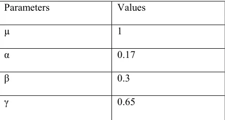
To perform the simulation we used the following parameters in table1.

Parameters Values

µ 1

α 0.17

β 0.3

[image:10.612.86.305.172.289.2]

γ 0.65

Table 1 .Parameters values of SEIR-SW model

For subfigures (a) and (b), when < k > is less than Ks, the disease disappears from the population, i.e.

there is a stability of the DFE, contrary to the case of < k > greater than Ks where the disease spreads in

the population as shown in the subfigures (c) and (d), and it corresponds to the results found previously (Theorem 4.5). This simulation transfers important information that is, self-quarantine and reducing the average number of neighbors in the society to less than the Ks, are effective strategies for

controlling epidemic diffusion.

6. CONCLUSION

In this paper to have studied the spreading of infectious disease in the small-world network, in order to better understand the structure of social contact networks and their role in epidemiology

.

We first studied the local and global stability of the Disease Free Equilibrium

E

0

=(s

*

,e

*

,i

*

)=(1,0,0)

and the Endemic Equilibrium

of the SEIR model within small world complex network, using the Lyapunov method, and expressed the results obtained using the average degree of distribution < k > of the network, and interpreted them according to a new threshold noted Ks.

 If the average degree of distribution

< k > < Ks then DFE is GAS;

 If the average degree of distribution

< k > > Ks then EE is GAS.

These results show the influence of the social aspect and the evolution of the network in the propagation of the epidemics, and in their asymptotic behaviors. And represent an important tool in decision-making and in the development of control strategies.

It implies that the disease can be eliminated from the community if <k> < _𝜶𝜷𝒂𝒃 , and it may be more practical for health decision makers to eradicate the disease and limit its spread. However we can’t deny that this work has some limitations, such for modeling disease caused by more than one strain of pathogen, such as tuberculosis [30], HIV [31], dengue fever [32] and other sexually transmitted diseases, that requires to be modeled with SIR and SEIR multi-strains models.

REFRENCES:

[1] Daniel Bernoulli. Essai d’une nouvelle analyse de la mortalité causée par la petite vérole et des avantages de l’inoculation pour la prévenir. Histoire de l’Acad. Roy. Sci.(Paris) avec Mém. des Math. et Phys. and Mém, 1760, pages 1–45. [2] Martin Dottori and Gabriel Fabricius. Sir model

on a dynamical network and the endemic state of an infectious disease. Physica A: Statistical Mechanics and its Applications, 2015, 434:25– 35.

[3] Jean-Pierre Françoise. La théorie de la stabilité. Oscillations en biologie: Analyse qualitative et modèles, 2005, pages 27–51.

[4] William Heaton Hamer. The Milroy lectures on epidemic disease in England: the evidence of variability and of persistency of type. Bedford Press, 1906.

[5] Xiao-Pu Han. Disease spreading with epidemic alert on small-world networks. Physics Letters A, 2007, 365(1):1–5.

[6] A. Iggidr. An introduction to ODE. INRIA Nancy-Grand Est LMAM, UPV-Metz, 2012. [7] Chunyan Ji and Daqing Jiang. Threshold

4280 [8] Daqing Jiang, Jiajia Yu, Chunyan Ji, and

Ningzhong Shi. Asymptotic behavior of global positive solution to a stochastic sir model.

Mathematical and Computer Modeling, 2011 54(1):221–232.

[9] William O Kermack and Anderson G McKendrick. A contribution to the mathematical theory of epidemics. In Proceedings of the Royal Society of London A: mathematical, physical and engineering sciences, volume 115, 1927, pages 700–721. [10] Guangzheng Li, Dinghua Shi, and Zhongzhi

Zhang. The discrete-time sis model in small-world networks. In Computer Science & Service System (CSSS), 2012 International Conference on IEEE, 2012 pages 1378–1380. [11] Michael Y Li and Liancheng Wang. A criterion

for stability of matrices. Journal of mathematical analysis and applications, 1998, 225(1):249–264.

[12] Ming Liu and Yihong Xiao. Modeling and analysis of epidemic diffusion within small-world network. Journal of Applied Mathematics, 2012.

[13] Mark EJ Newman, Steven H Strogatz, and Duncan J Watts. Random graphs with arbitrary degree distributions and their applications. Physical review E, 2001, 64(2):026118.

[14] Romualdo Pastor-Satorras and Alessandro Vespignani. Epidemic dynamics and endemic states in complex networks. Physical Review E, 2001, 63(6):066117.

[15] Ronald Ross. The prevention of malaria. John Murray; London, 1911.

[16] Mohammad A Safi and Salisu M Garba. Global stability analysis of seir model with holling type II incidence function. Computational and mathematical methods in medicine, 2012. [17] G. Sallet. Introduction à l’Epidémiologie

Mathématique et aux Systèmes Dynamiques. Equipe Projet INRIA MASAIE INRIA Nancy Grand Est, 2012.

[18] Funda Samanlioglu, Ayse Humeyra Bilge, and Onder Ergonul. A susceptible-exposed-infected-removed (seir) model for the 2009-2010 a/h1n1 epidemic in istanbul. arXiv preprint 2012, arXiv:1205.2497.

[19] Jari Saramäki and Kimmo Kaski. Modelling development of epidemics with dynamic small-world networks. Journal of Theoretical Biology, 234(3):413–421, 2005.

[20] MM Telo da Gama and A Nunes. Epidemics in small world networks. The European Physical Journal BCondensed Matter and Complex Systems, 50(1):205–208, 2006.

[21] Pauline Van den Driessche and James Watmough. Reproduction numbers and sub-threshold endemic equilibria for compartmental models of disease transmission. Mathematical biosciences, 180(1):29–48, 2002.

[22] Yi Wang, Jinde Cao, Ahmed Alsaedi, and Bashir Ahmad. Edge-based seir dynamics with or without infectious force in latent period on random networks. Communications in Nonlinear Science and Numerical Simulation, 2017, 45:35–54.

[23] Duncan J Watts and Steven H Strogatz. Collective dynamics of ‘small-world’networks. Nature, 1998, 393(6684):440–442.

[24] Na Yi, Qingling Zhang, Kun Mao, Dongmei Yang, and Qin Li. Analysis and control of an seir epidemic system with nonlinear transmission rate. Mathematical and computer modeling, 2009, 50(9-10):1498{1513.

[25] Yi Wang, Jinde Cao, Ahmed Alsaedi, and Bashir Ahmad. Edge-based seir dynamics with or without infectious force in latent period on random networks. Communications in Nonlinear Science and Numerical Simulation, 2017, 45:35–54.

[26] Syafruddin Side, Wahidah Sanusi, Muhammad Kasim Aidid, and Sahlan Sidjara.

Global stability of sir and seir model for tuberculosis disease transmission with lya-punov function method. Asian. J. Appl. Sci, 2016, 9:87{96.

[27] Azizeh Jabbari, Carlos Castillo-Chavez, Fereshteh Nazari, Baojun Song, and Hossein Kheiri. a two-strain tb model with multiple latent stages. Math. Biosci. Eng, 2016 13:741{785.

[28] Ebenezer Bonyah, Muhammad Altaf Khan, KO Okosun, and Saeed Islam. A theoretical model for zika virus transmission. PloS one, 2017, 12(10):e0185540.

[29] Bentaleb D, Amine S. Lyapunov function and global stability for a two-strain seir model with bilinear and non-monotone incidence. International Journal of Biomathematics 2019. [30] JE Golub, S Bur, WA Cronin, S Gange, N

4281 [31] Duane J Gubler. Epidemic dengue and dengue

hemorrhagic fever: a global public health problem in the 21st century. In Emerging infections 1, pages 1{14. American Society of Microbiology, 1998.