A ROBUST FRAMEWORK TO DETECT MOVING VEHICLES IN DIFFERENT ROAD CONDITIONS IN INDIA

23

HYBRID ARTIFICIAL BEE COLONY ALGORITHM WITH

MULTI-USING OF SIMULATED ANNEALING ALGORITHM

AND ITS APPLICATION IN ATTACKING OF STREAM

CIPHER SYSTEMS

1_{MAYTHAM ALABBAS,} 2_{ABDULKAREEM H. ABDULKAREEM}

1,2_{University of Basrah, Department of Computer Science, Basrah, Iraq}

E-mail: 1_{[email protected],} 2_{[email protected],}

ABSTRACT

A new hybrid evolution algorithm (ABC-SA), i.e. artificial bee colony algorithm (ABC) with multi simulated annealing (SA) using, is presented. In ABS-SA procedure, the ABC provides a global search and the SA algorithm provides local search. SA processes are used to improve the original ABC algorithm into two different manners: (i) repair the initial food sources of ABC, which is generally carried out randomly, in order to look for promising areas; and (ii) selecting a candidate food source because SA can escape from local optimum point by accepting worse solutions at a particular probability in the neighbor searching period.

The ABC-SA algorithm has been applied to break a number of linear and nonlinear stream cipher systems, which is one of the hard electronic cipher systems because of high security and difficulty in breaking it. The current findings are encouraging. Comparison of the results indicated that in most cases the ABC-SA algorithm outperforms the original ABC algorithm.

Keywords: Artificial Bee Colony Algorithm, Simulated Annealing, Hybrid algorithm, Stream Cipher

System

1. INTRODUCTION

Optimization plays a key role in many fields and applications. A number of algorithms have been offered in this regard such as artificial bee colony (ABC) [1], simulated annealing (SA) [2], genetic algorithm (GA) [3], particle swarm optimization (PSO) [4], differential evolution (DE) [5], and others [6]. Each of these algorithms has good and weak points that make them work good in a set of problems and weak in some other problems. Therefore, one popular way to cover the weakness of each algorithm and have a better performance than can be obtained by any of them in isolation is by hybridizing them. Many authors in the literature have proposed different hybridizing strategies in this regard. Some of these strategies are briefly explained in the following lines.

Juang [7] combined GA with PSO, named HGAPSO. The author applied HGAPSO algorithm

24 ABC version, named HABC-SA, to solve the travelling salesman problem (TSP). The crossover and mutation operators are applied to do a local search (i.e. complete neighbourhood search) and the SA is imported to increase the food sources diversity. Yurtkuran and Emel [14] applied a new solution acceptance rule instead of greedy selection between old and new solutions with the acceptance probability of worse candidate solutions. The authors also employ three distinct search equations with varying intensification and diversification abilities. Rahmi et al. [15] proposed a hybrid SA-GA algorithm to solve the distribution problem. The SA algorithm based on the crossover process is utilized to generate the initial population for GA. The current work is a step forward in this regards. The novelty of this work is utilizing the advantages of SA into two different places: (i) using SA based on the uniform crossover to improve the initial (randomly generated) food source set of the ABC; (ii) applying the Yurtkuran and Emel [14]'s acceptance rule in place of greedy selection through only the employed bee phrase to improve the diversification.

The rest of this paper is organized as follows. Section 2 outlines two optimization algorithms, ABC and SA algorithms. Section 3 describes a new hybridized ABC-SA algorithm. A summary of the stream cipher systems and modeling of current work are given in Section 4. Section 5 presents the results of the experiments we have carried out on various stream cipher system parameters and compares the stability and rate of convergence of the two optimization algorithms on this problem. Section 6 presents a summary discussion.

2. OPTIMIZATION ALGORITHMS

In the current work, two popular optimization algorithms are used that are artificial bee colony algorithm (ABC) and simulated annealing (SA). The reasons behind the selection of these two algorithms are because these algorithms have verified to be effective and powerful in search processes, and have gotten (near) optimal solutions, making them approved for solving large and complex problems.

2.1 Artificial bee colony (ABC) algorithm

In the ABC algorithm, the artificial bees’ colony consists of three groups [16]: (1) employed bees going to the food source, which is a feasible solution to the problem to be optimized, that they have visited previously; (2) onlookers waiting to

choose a food source; and (3) scouts carrying out random search. In the colony, the first half includes the employed artificial bees and the second half consists of the onlookers and scouts. Both the number of employed bees and the number of food sources are equal. The employed bee of an abandoned food source becomes a scout. The pseudo-code of the original ABC algorithm is shown in Figure 1 [17].

ABC follows three steps during each cycle: (i) moving both the employed and onlooker bees onto the food sources; (ii) calculating their nectar amounts (fitness value); and (iii) determining the scout bees and then moving them randomly onto the possible food sources.

The ABC algorithm has been widely used in many optimization applications since it is easy to implement and has fewer control parameters than the other popular algorithms such as GA.

2.2 Simulated Annealing algorithm

25

3. HYBRIDARTIFICIALBEECOLONYAND

SIMULATED ANNEALING (ABC-SA)

ALGORITHM

Each of the ABC and SA algorithms has good and weak points that may make them work well in some problems and not well in some others. The ABC-SA algorithm combines the advantages of faster computation of the original ABC algorithm with the robustness of SA to exploit the unique advantage of each algorithm, reduce its computational cost, and increase the global search capability.

The current ABC-SA algorithm applies SA into different manners:

(i) In its early search stages, the hybrid algorithm focuses mostly on looking for promising areas by applying SA processes to improve the initial set of food source (population) of the ABC that randomly generated. After the initial population is generated and evaluated, the SA is performed for each solution (see Figure 3, step 4). During the SA process, we used the GA crossover operator, uniform crossover (UX), which exchanges building blocks between two individuals with a specific probability to create a new solution. Next, the best solutions obtained from the SA are the starting population for the next cycles;

(ii) When the search space promising areas have been well identified, the hybrid ABC-SA algorithm allows higher exploitation levels by selecting a candidate food source based on the SA idea in order to keep the balance of convergence speed and convergence precision. SA has the ability to escape from local optimum solution, especially when hybrid with other algorithms since it accepts worse solutions at a particular probability in the neighbor-searching period.

To achieve this, we follow the solution acceptance rule that proposed by Yurtkuran and Emel [14] (see Figure 3, step 8), but in place of the greedy selection process in employed bee phase only, not like [14] for both employed bee phase and onlookers bee phase, because it is responsible for diversification. The worst solution may have a chance to be accepted as the new solution according to acceptance probability. By doing this, the process may jump out of local optimum and explore the search space in an active way.

In hybrid ABC-SA algorithm, if the worst solution is generated during the employed bee phase, it is processed using the following: if

the generated solution vij has an equal or better fitness f(vij) than the fitness of old source f(xij),

then vij is chosen as the candidate solution.

Otherwise, the new solution vij is accepted if a random number within the range [0,1] is less than a probability Pa that is explained in Equation 1, else xij is chosen as the candidate

solution.

Pa= P0 ((1+cos((iter/MaxIter) ) × 0.5), (1)

where P0 is the initial probability, iter and

MaxIter denote the current and maximum

iteration number. As can be seen from Equation 1, the acceptance probability Pa is nonlinearly decreased from P0 to 0 during the search process. The range of Pa is [0, P0]. The trial counter is incremented, regardless of a worse candidate solution is accepted or not.

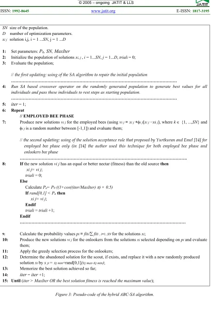
The hybrid ABC-SA algorithm may be able to cover each component weaknesses and has a better performance than its component. The pseudo-code of this algorithm is shown in Figure 3.

4. APPLICATION

a. Stream cipher systems

In order to check the effectiveness of the hybrid ABC-SA algorithm, we tested it for breaking stream cipher systems (SCs) with a known plaintext attack, which is a complicated problem and challenging. SCs convert a plaintext to a ciphertext one bit at a time. The output bits stream

(K1, …, Ki) of the keystream generator is XORed with plaintext bits stream (P1, …, Pi) to produce ciphertext bits (C1, ..., Ci). At the decryption end, the ciphertext bits are XORed with an identical keystream to recover the plaintext bits as shown in Figure 4 [18].

26 The linear feedback shift register (LFSR) is the main component of the keystream generator that consists of two parts: the shift register and feedback function as shown in Figure 5.

Figure 5: Linear Feedback Shift Register (LFSR) System

As it can be seen in Figure 5, all the bits (bn,…,b1) in the shift register are shifted to the right. The new left-most bit is computed as a function of the other bits [2]. The period of the shift register is the length of the output sequence before it starts repeating. Moreover, more than one LFSR may generate a binary sequence and the short one that generating this sequence is known as the linear equivalence. The LFSR characteristics polynomial is named the minimal polynomial with degree equal to the linear equivalence. In addition to the number of LFSR bits is equal to that of the linear equivalence of the sequence generated from that register.

b. Modeling

In the current experiments, the main goal of using hybrid ABC-SA algorithm is to find the linear equivalence of a given key stream through finding: Initial state, feedback function, and shift register length, with knowing part of the plain text that a cipher text and part of it are known.

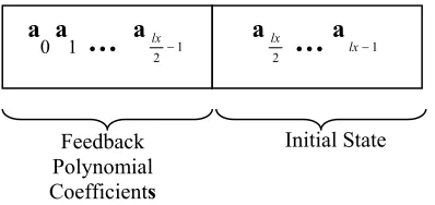
The food source is represented as a binary string (a0,…,aLx) with variable lengths and an even length, Lx. It is divided into two equal parts, one for the feedback function (a0,…,a(Lx/2)-1) and the other for the initial state of the LFSR equivalent to the attacked generator (a(Lx/2),…,aLx-1) as shown in Figure 6.

Figure 6: Current food source structure

The nectar (fitness) value is the percentage matching between the knowing part of the plaintext and the generated text as the number of matched bits between them when the highest matching is better as explained in the following equation.

fitness(X)= (



 n

i1

(1-|Ai-Bi|)/n)×100, (2)

where x is an individual, n is the length of the knowing part of the plaintext, Ai is ith _{bit of the}

knowing part of the plaintext, and Bi is ith _{bit of the}

generated text. The best value for fitness is equal to n, which means the knowing part of the plaintext and the generated text are identical.

We used the hybrid ABC-SA algorithm with the following settings:

 The colony size is 20 solutions;

 The percentages of onlooker bees and employed bees were 50% of the colony;

 The number of scout bees was selected as one;

 The maximum number of cycles for foraging is 1000 cycles. The algorithm terminates when either a maximum number of cycles has been produced, or a fitness value of an individual equals to the length of the knowing part of the plaintext.

5. EXPERIMENTAL RESULTS

In this section, we will answer the question as to which algorithm (original ABC algorithm or hybrid ABC-SA algorithm) works best for our task? To answer the above question, we need to answer two main subsidiary questions: (i) how good a value does it produce?; and (ii) how quickly does it produce this value?

Feedback Polynomial Coefficients

a

0

a

…

a

lx

a

2 lx

…

a

1



lx

27 In general, to answer the above questions, we have to experiment to find out, since they are applications-independent. Generally, the most serious challenge in the use of optimization algorithms is concerned with the quality of the results, in particular, whether or not an optimal solution is being reached. One way of providing some degree of insurance is to compare results obtained for N times under different seeds of the initial population. We, therefore, performed both algorithms three times with different random seeds for each run and the same initial seed for both algorithms.

To assess the reliability of the original ABC and hybrid ABC-SA algorithm, we calculate the average performance (fitness) and cycles of them for the whole set of runs. A more reliable algorithm should produce (in our case) a higher value for mean, preferably near to the global maximum one.

In the current work, four diverse experiments are performed.

Experiment 1

In the first experiment, a linear stream cipher is chosen with different LFSR lengths and constant length of known key stream equals to 20-bit. The results are shown in Table 1.

As it can be seen from the results presented in Table 1, the hybrid ABC-SA algorithm the outperforms original ABC algorithm in all runs in terms of the quality of the results (average of the reliability of results is 100% compared to 88% for the original ABC) and the number of cycles (the hybrid ABC-SA algorithm takes less average number of cycles than the original ABC algorithm for all tests). The original ABC algorithm also fails to get correct results when LFSR length more than 7. Besides that, whenever the length of the shift register increases (key size), the average number of cycles increases too.

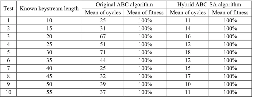
Experiment 2

This experiment is for examining the effect of the known key stream length on the convergence speed. Linear stream cipher with the shift register of length 5 bits is chosen. Table 2 shows the results of this experiment.

The first thing to note in Table 2 that the hybrid ABC-SA algorithm outperforms the original ABC algorithm in terms of the number of cycles for the most length of the known key stream. Both algorithms are fully reliable.

Experiment 3

In the third experiment, two known nonlinear stream cipher systems, which are the Hadmard system (Figure 7) and the Bruer system (Figure 8), are adopted. The GCD(k1, …, kn) should be equal to 1. The results of this experiment are illustrated in Table 3 for the known keystream length equals 15-bits.

Figure 7: General diagram of Hadmard system.

Figure 8: General diagram of Bruer system.

28 45 55 65 75 85 95 105

1 _{13 25 37 49 61 73 85 97}

10 9 12 1 13 3 14 5 15 7 16 9 18 1 19 3 20 5 21 7 22 9 24 1 25 3 26 5 27 7 28 9 Fi tn e ss Cycle The performance of ABC Best fitness Mean fitness Experiment 4

For the purpose of comparing the behavior of the hybrid ABC-SA algorithm more clearly with the behavior of the original ABC, we used ‘performance graphs’ [19]. This a graph is a curve showing the best individual performance in the population in addition to the average performance of the entire population over the chosen number of cycles.

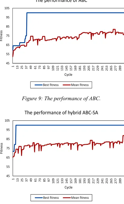
Figure 9: The performance of ABC.

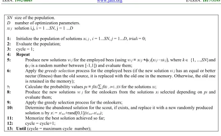
Figure 10: The performance of hybrid ABC-SA.

Figures 9 and 10 demonstrate plots of the best and average values of the fitness across 100 cycles for both the original ABC algorithm and the hybrid ABC-SA algorithm respectively, where both algorithms have been run with the same initial population and the same colony size (population) of 20. The other settings are the same for both algorithms. In these graphs, the x-axis indicates how many cycles have been created and evaluated at the particular point in the run, and the y-axis represents the fitness value at that point.

The first thing to note in Figure 9 is that the best fitness is around doubled over the 300 cycles. The best fitness curve rises slowly at the beginning of the experiment (until cycle 39), but stays flat after cycle 40 until the end, with very small increments at cycles 2, 20, 34, 36 and 39 respectively. This algorithm gets the optimal fitness at cycle 39. The average fitness curve rises nearly gradual and the population converges nearly on the best solution at the beginning of the experiment (until cycle 39), but then it shows erratic behavior between 68 and 79 (apart from very minor increments at cycles 19-22).

On the other hand, the best fitness curve obtained by the hybrid ABC-SA algorithm in Figure 10 shows an even steeper improvement at the beginning of the experiment (until cycle 9), which converges very quickly to the best fitness but stays flat for the end. The average fitness curve starts with gradual improvement and the population converges nearly on the best solution at the beginning of the experiment (until cycle 8), and then it shows erratic behavior between 72 and 82 (again apart from very minor decrements at cycles 15, 24 and 59 respectively and very minor increments at cycles 210-214 and 298-300 respectively). Besides, the average fitness obtained by the hybrid algorithm is a higher value than that for original ABC by around three.

To conclude, as it can be seen from the results presented in experiments 1-4, hybrid ABC-SA algorithm outperforms ABC in all runs in terms of the quality of the results (this is the answer for the first question) and the convergence speed of the hybrid ABC-SA is better than ABC under the same conditions (this is the answer for the second question).

The present findings of these experiments are encouraging and prove that using selection process for employed bee phase differ from that used in onlookers bee phase will explore the search space in an active way because it takes the advantages of both selection processes. Further work in this regard would be very worthwhile.

6. CONCLUSIONS

A new hybridized artificial bee colony algorithm with simulated annealing (ABC-SA) is presented in the current work. To keep the balance of convergence speed and convergence precision, SA is repaired the initial food sources of ABC and

45 55 65 75 85 95 105

1 _{13 25 37 49 61 73 85 97}

29 is imported to select the candidate solution with a probability of acceptance to select the worst solution during the employed bee phase instead of the greedy selection that is used in the original algorithm.

The hybrid ABC-SA algorithm is tested on breaking stream cipher systems with a known plaintext attack. The algorithm should find the shortest LFSR which generates a sequence of key stream knowing part of it. We have carried out a number of experiments on linear/non-linear stream cipher system using original ABC algorithm and hybrid ABC-SA algorithm.

The simulation results of these experiments show that the performance of the hybrid ABC-SA algorithm, in terms of the quality of results, convergence speed and avoidance of local maxima, is better than the original ABC algorithm under the same conditions. Its performance is very good in terms of the local and the global optimization due to the selection schemes employed and the neighbor production mechanism used. Moreover, the nonlinear stream cipher systems need more time for breaking it than the linear one because the degree of nonlinearity is greater. Consequently, it can be concluded that the hybrid ABC-SA algorithm based approach can successfully be used in the optimization of breaking linear and nonlinear stream cipher systems

We intend to investigate other techniques between the ABC algorithm and the SA algorithm. Further experimental investigations are needed to hybridizing other optimization techniques, such as PSO, DE, GA, and others.

Another interesting task for future exploration is testing a stacking technique between two algorithms.

REFERENCES:

[1] D. Karaboga and B. Basturk, "A powerful and efficient algorithmfor numerical function optimization: artificial bee colony (ABC) algorithm," Journal of Global Optimization,

vol. 39, pp. 459–471, 2007.

[2] A. Scollen and T. Hargraves, Simulated Annealing: Introduction, Applications and Theory: Nova Science Pub. Inc., 2018.

[3] L. Jacobson and B. Kanber, Genetic Algorithms in Java Basics: Springer, 2015. [4] M. Clerc, Particle Swarm Optimization, 1st

ed.: Wiley-ISTE, 2006.

[5] K. Price, R. Storn, and J. Lampinen,

Differential Evolution: A Practical Approach

to Global Optimization Springer-Verlag

Berlin, 2011.

[6] D. Simon, Evolutionary Optimization Algorithms, 1st ed.: Wiley, 2013.

[7] C. F. Juang, "A hybrid of genetic algorithm and particle swarm optimization for recurrent network design," Secondary A hybrid of genetic algorithm and particle swarm optimization for recurrent network design,

vol. 34, pp. 997-1006, 2004.

[8] A. Chen, G. Yang, and Z. Wu, "Hybrid discrete particle swarm optimization algorithm for capacitated vehicle routing problem," Secondary Hybrid discrete particle swarm optimization algorithm for capacitated vehicle routing problem, vol. 7, pp. 607-614, 2006.

[9] W. Xia and Z. Wu, "An effective hybrid optimization approach for multi-objective flexible job-shop scheduling problems,"

Secondary An effective hybrid optimization approach for multi-objective flexible job-shop scheduling problems, vol. 48, pp. 409-425, 2005.

[10] B. Niu and L. Li, "A novel PSO-DE-based hybrid algorithm for global optimization,"

Secondary A novel PSO-DE-based hybrid algorithm for global optimization, pp. 156-163, 2008.

[11] E. Mirsadeghi and M. S. Panahi, "Hybridizing Artificial Bee Colony with Simulated Annealing," International Journal of Hybrid Information Technology, vol. 5, pp. 11-18, 2012.

[12] R. Agasthiya and E. Latha Mercy, "A Hybrid ABC-GA Solution for the Economic Dispatch of Generation in Power System,"

International Journal of Computer Applications, pp. 5-10, 2013.

[13] P. Shi and S. Jia, "A Hybrid Artificial Bee Colony Algorithm Combined with Simulated Annealing Algorithm for Traveling Salesman Problem," presented at the International Conference on Information Science and Cloud Computing Companion, Guangzhou, China, 2014.

[14] A. Yurtkuran and E. Emel, "An Enhanced Artificial Bee Colony Algorithm with Solution Acceptance Rule and Probabilistic Multisearch," Computational Intelligence and Neuroscience, p. 13, 2016.

30

Telecommunication, Electronic and Computer Engineering, vol. 9, pp. 177-182, 2017.

[16] D. Karaboga, B. Gorkemli, C. Ozturk, and N. Karaboga, "A comprehensive survey: artificial bee colony (ABC) algorithm and applications," Artificial Intelligence Review,

vol. 42, pp. 21–57, 2014.

[17] B. Akay and D. Karaboga, "A Modified Artificial Bee Colony Algorithm for Real-Parameter Optimization," Information Sciences, vol. 192, pp. 120-142, 2012. [18] C. Paar and J. Pelzl, Understanding

Cryptography: A Textbook for Students and Practitioners: Springer Berlin Heidelberg, 2010.

31

SN size of the population.

D number of optimization parameters.

xi j solution i,j, i = 1 ...SN, j = 1 ...D

1: Initialize the population of solutions xi, j , i = 1...SN, j = 1...D, triali = 0;

2: Evaluate the population;

3: cycle = 1;

4: Repeat

5: Produce new solutions vi j for the employed bees (using vi j = xi j +i j(xi j −xk j), where k  {1, ...,SN}and i j is a random number between [-1,1]) and evaluate them;

6: Apply the greedy selection process for the employed bees (if the new solution vi j has an equal or better

nectar (fitness) than the old source, it is replaced with the old one in the memory. Otherwise, the old one is retained in the memory);

7: Calculate the probability values pi = fiti/fiti , i=1..SN for the solutions xi;

8: Produce the new solutions vi j for the onlookers from the solutions xi selected depending on pi and

evaluate them;

9: Apply the greedy selection process for the onlookers;

10: Determine the abandoned solution for the scout, if exists, and replace it with a new randomly produced solution xi by xj

i= xjmin+rand[0,1](xjmax-xjmin);

11: Memorize the best solution achieved so far;

12: cycle = cycle+1;

13: Until (cycle = maximum cycle number);

Figure 1: Pseudo-code of the original ABC algorithm.

1: Initialize Scurrent; 2: T= <some high value>;

3: While T > <specific value>

4: For iteration= 1 to <some constant value>

5: Scandidate = Scurrent

6: E = Error(Scandidate) - Error(Scurrent) 7: If E ≤ 0

8: Scurrent = Scandidate 9: Else

10: prob = e (-E/T) 11: If rand(0,1) ≤ prob

12: Scurrent = Scandidate 13: Endif

14: Endif

15: Endfor

16: decrement T

17: Endwhile

32

SN size of the population.

D number of optimization parameters.

xi j solution i,j, i = 1 ...SN, j = 1 ...D

1: Set parameters: P0, SN, MaxIter

2: Initialize the population of solutions xi, j , i = 1...SN, j = 1...D, triali = 0;

3: Evaluate the population;

// the first updating: using of the SA algorithm to repair the initial population

………

4: Run SA based crossover operator on the randomly generated population to generate best values for all

individuals and pass these individuals to rest steps as starting population.

……… 5: iter = 1;

6: Repeat

// EMPLOYED BEE PHASE

7: Produce new solutions vi j for the employed bees (using vi j = xi j +i j(xi j −xk j), where k  {1, ...,SN} and i j is a random number between [-1,1]) and evaluate them;

// the second updating: using of the solution acceptance rule that proposed by Yurtkuran and Emel [14] for employed bee phase only (in [14] the author used this technique for both employed bee phase and onlookers bee phase

………. 8: If the new solution vi j has an equal or better nectar (fitness) than the old source then

xi j= vi j;

triali = 0;

Else

Calculate Pa= P0 ((1+cos((iter/MaxIter) ) × 0.5) Ifrand[0,1] < Pathen

xi j= vi j; Endif

triali = triali +1;

Endif

………

9: Calculate the probability values pi = fiti/fiti , i=1..SN for the solutions xi;

10: Produce the new solutions vi j for the onlookers from the solutions xi selected depending on pi and evaluate

them;

11: Apply the greedy selection process for the onlookers;

12: Determine the abandoned solution for the scout, if exists, and replace it with a new randomly produced solution xi by x ji = xj min+rand[0,1](xj max-xj min);

13: Memorize the best solution achieved so far;

14: iter = iter +1;

15: Until (iter >MaxIter OR the best solution fitness is reached the maximum value);

33

Table 1: Comparison between classic ABC and hybrid ABC-SA algorithm for three runs, different LFSR lengths with constant known keystream length

Test LFSR length Original ABC algorithm Hybrid ABC-SA algorithm Mean of cycles Mean of fitness Mean of cycles Mean of fitness 1 4 22 100% 12 100% 2 5 38 100% 15 100% 3 6 244 100% 16 100% 4 7 177 100% 36 100% 5 8 1000 69% 55 100% 6 9 1000 99% 62 100% 7 10 1000 90% 143 100% 8 11 1000 77% 366 100% 9 12 1000 81% 421 100% 10 13 1000 65% 513 100%

Table 2: Comparison between original ABC and hybrid ABC-SA algorithm for three runs, constant LFSR length with different known keystream lengths

Test Known keystream length Original ABC algorithm Hybrid ABC-SA algorithm Mean of cycles Mean of fitness Mean of cycles Mean of fitness

1 10 25 100% 11 100%

2 15 31 100% 14 100%

3 20 67 100% 16 100%

4 25 51 100% 12 100%

5 30 71 100% 18 100%

6 35 44 100% 12 100%

7 40 25 100% 15 100%

8 45 32 100% 17 100%

9 50 39 100% 10 100%

10 55 37 100% 11 100%

Table 3: Comparison between original ABC and hybrid ABC-SA algorithm for three runs, two non-linear stream cipher systems