Munich Personal RePEc Archive
Validating Prediction of a CGE Model of
India: An Introspection
Pohit, Sanjib and Chadha, Rajesh and Pratap, Devender and
Ghosh, B,K.
NCAER
1999
Online at
https://mpra.ub.uni-muenchen.de/94860/
Validating Prediction of a CGE Model of India:
An Introspection
Sanjib Pohit, Rajesh Chadha, B.K. Ghosh, and Devender Pratap
*ABSTRACT
Although computable general equilibrium (CGE) models have been used extensively to evaluate the potential impact of economic reforms, few efforts have been made to assess the predictive power of the models. This paper attempts to test the performance of one such model, viz., Chadha, Pohit, Deardorff and Stern’s study of India’s unilateral trade/domestic policy reforms in the 1990s. Our model does not incorporate many of the rigidities/features of the Indian economy. Nevertheless, our model can perform quite well at simulating, if not forecasting, actual changes in sectoral output and exports
Address correspondence to:
Rajesh Chadha/ Sanjib Pohit / Devender Pratap
National Council of Applied Economic Research (NCAER) Parisila Bhawan,
11-Indraprastha Estate New Delhi-10002 India
Tel. (91-11) 3317860-68 Fax (91-11) 3327164
Email: [email protected]; [email protected]; and [email protected]
*
2
1. INTRODUCTION
The product of many CGE model-building exercise is often seen as simply another economic
model to add to a collection rather the birth of an important tool capable of answering economic
questions. There are many reasons for the current level of skepticism surrounding CGE modeling
effort. In implementing a CGE model, one is required to make many assumptions regarding data base,
behavioral equations, and parameters. While CGE modelers may find that most of these assumptions
are necessary and defensible, this provides little assurance to consumers of results. Of more interest to the modeler’s clients is whether a model is capable of producing a proven set of results deemed accurate and reliable. Thus, an exercise aimed at evaluating a model based on its predictive
performance seems well placed. Of late, few attempts have been made in validating results of CGE
models of developed countries.1 In this spirit, this paper makes an attempt to test the forecast changes
due to Indian trade liberalization in the nineties as modeled by Chadha, Pohit, Deardorff and Stern
(1998a, 1998b) in their 34-sector India CGE model.
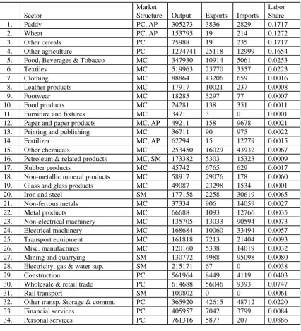
This India Model is a single-country, multi-sectoral CGE model.2 India is modeled to produce,
consume and trade 33 tradable goods. In addition, there is one non-traded sector, rail transport. The
sectors of the model, their market structure along with key sectoral economic indicators of the Indian
economy in the base year of our model, viz. 1989-90, is shown in Table 1.
The market structure in 29 of the 34 sectors is modeled as either perfectly competitive or
monopolistically competitive, depending on the degree of scale economies in production. All the
tradable sectors are assumed to be characterized by some degree of product differentiation..
There are two factors of production namely, labor and capital in the non-agricultural sectors of
model. However, land is also considered as an additional factor of production in the four agricultural
sectors. All factors of production are assumed to be perfectly mobile across sectors, except that all
capital is assumed to be immobile into and out of the state monopoly sectors. Returns to land, capital
(in sectors across which it is mobile), and labor are determined to equate factor demand to an
exogenous supply of each factor. The aggregate supplies of labor, capital, and agricultural land are
assumed to remain fixed so as to abstract from macroeconomic considerations involving, for
example, determination of investment, since our focus is on the intersectoral allocation of resources. India’s merchandise imports/exports are subject to tariffs and non-tariff barriers (NTBs). NTBs are incorporated by endogenously solving for the ad valorem tariff-equivalent rate that would hold
imports/exports within each product category covered by NTBs at a pre-determined level. Tariff rates
are aggregated according to the sectors specified in Table 1.
In our model we assume that aggregate expenditure varies endogenously to hold aggregate
1
3
employment constant. In addition to above closing rule, we need to specify several variables to be
exogenous for obtaining the model solution. Typically, these are the policy inputs to the model.
3. THE SCENARIOS AND DATA
The paper by Chadha et al (1998a) reported different scenarios on changes in tariffs/NTBs
relating to exports/imports/output under following alternative assumptions: (1) the economy retains
certain product market imperfections (state monopolies and administered prices) as these existed in
1989-90; (2) the economy is free from such distortions. In that paper, we reported two sets of policy
shocks depending on our assumption regarding the path of reforms that were likely to take place
between 1989-90 to 1995-96 and between 1989-90 to 1998-99.3
After seven years of economic reforms, it is now evident that the most of the domestic reforms are
yet to be undertaken. Consequently, if we are to validate our predictions against actual, it seems to be
more appropriate to compare our model results keeping status quo as far as domestic reforms are
considered. This is more so since the data availability constraint us to compare our predictions
against actual outcomes for the period 1989-89 to 1994-95.4
In the original run of the model, we have applied the following shocks for the simulation
pertaining to the period 1989-90 to 1995-96.
a. Reduction in Import/Export tariffs: We have reduced the import tariff as per the recommendation of
Chelliah Committee.5 Since export taxes were already negligible in 1989-90, they were not shocked.
b. Reduction in NTBs on Imports/Export: The existing NTBs (1989-90) on imports/exports were
assumed to be partially relaxed so as to permit a specified per cent increase in the imports/exports that
had been constrained. This was implemented in the model by increasing the level of imports (or
exports) that were under some kind of quantitative restriction for the sectors subject to import NTBs (or
export NTBs). The estimated increases in imports from relaxation of NTBs for agricultural, consumer
and other goods including services are respectively 10% 25% and 75%. On the other hand, we have
assumed increases in exports from relaxation of NTBs on exports for agricultural sectors as 25% and for
the remaining sectors as 50%. While these estimates are not based on any actual declared numbers,
we have tried to incorporate the implicit intentions in various policy announcements whereby the
imports of agricultural and consumer goods are likely to remain more restricted than the other sectors of
the economy.6
c. Rationalization of Indirect Taxes: In the original runs of the model, we had reduced the subsidies
2
The technical details and equations of the model are available in Chadha, Pohit, Deardorff, and Stern (1998b).
3
It should be mentioned that the breakup of the time period was a bit arbitrary.
4
The data problem is discussed later.
5
4
(net indirect taxes) in the following sectors--- 4 agricultural sectors; fertilizer; and electricity, gas, and
water supply sectors --- by 5% and had decreased excise duties in the remaining sectors by 5%.
In retrospect, we find from the latest available data/publication that our assumption regarding
deepening of trade liberalization by the year 1994-95 was completely off marks in certain sectors. For
example, there was no relaxation on NTBs in service sectors during the period 1989-90 to 1994-95. The
same holds true for the four agricultural sectors.7 On the other hand, actual import tariff rates in 1995/96
were by and large in line with Chelliah committee recommendations (used for the model run).8
In the light of these observations, it seems appropriate to modify the shocks for the validation
exercise. Accordingly, the following modifications to the shocks were made:
(a) we assume status quo to be maintained in the NTBs in the agricultural and the service sectors,
(b) other indirect tax rates are modified on the basis of actual changes between the years 1989-90 and
1994-95.9
The original model requires estimates of various types of elasticity measures, viz. demand elasticities
of exports and imports and elasticites of substitution between factors of production and between
varieties of goods. We have used the same values of the parameters for this exercise.10
Given the fact that revised shocks are given only to 23 manufacturing sectors, our validation exercise
is carried out only for three major variables, namely, output, exports and imports, of these sectors for
which we could generate sectoral data sets for the years 1989-90 and 1994-95.
4. EVALUATION OF INDIA MODEL RESULTS
In order to measure the goodness of fit of the predicted changes in selected variables, we have
considered for our analysis following two measures of goodness of fit----
1. weighted correlation (r), between the predicted and observed vectors of changes:
i i i i i i i i i i
y
w
y
w
y
y
w
r
2 2 2 2 2, where wi , the weight for sector i, is derived from the base year
(1989-90) values of the variable. This measure rewards predictions that have the right signs and relative
magnitudes, but it does not take into account the absolute magnitude of the changes.
2. adjusted R2 resulting from the weighted regressions of the predictions against actual outcomes:
6
See Panagariya (1999), Export/Import Policy document of Government of India.
7
The shares of restricted imports to total imports for paddy, wheat, other cereals were 100% in 1994-95. There was only marginal relaxation in NTBs in the other agricultural sector (see Chadha and Pohit, 1998c, for details).
8
See Pursell (1996), RIS (1998) for details.
9
The rates are computed using our constructed inter-industry transaction tables, concorded to our sectors, for the years 1989-90 and 1994-95.
10
5
i i i i
i
y
w
w
y
1
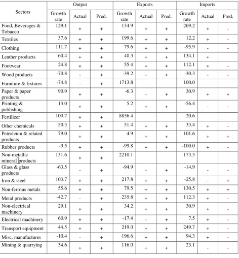
Before we begin our evaluation exercise, it will be worthwhile to see the sectoral growth rates of
output, imports, and exports for manufacturing sectors of our economy (see Table 2a). As Table 2a shows, growth rates of sectoral output lie between –70% to 120%. The same is not true of imports and exports. As this table shows, several sectors, notably, furniture and fixtures, fertilizer, and non-metallic
mineral products exhibit abnormally high/low growth rates of exports/ imports due to a low base factor.
It is understandable that the predictions from no model can match such high sectoral growth. For this reason, we have dropped above 3 sectors for validating import/export’s growth rates.
Table 2a displays actual and predicted direction of change of output, imports, and exports between the years 1989-90 and 1994-95. A ‘+’ (or ‘-‘) under the heading actual/predicted for a sector in Table 2a implies that the corresponding sector registered positive (or negative) rate of growth during the period.
According to Table 2a, the model correctly predicts the observed direction of change of output in 18 out
of 23 sectors under study. That is, our prediction of output change is off the target in 22% of cases.
With regard to export, our model could correctly infer the direction of change in 16 out of 20 sectors.
As far as imports are concerned, our inference is less accurate: we could predict correctly in 8 out of 20
sectors.
The above discussion suggests that our model predicts moderately well the observed direction of
change. How well are these predictions in terms of standard measures of goodness of fit? Table 2b
summaries our findings. As this table shows, the weighted correlation between the predicted and
observed changes of output is 0.56. On the other hand, the goodness of fit, as measured by adjusted R2
of the regression of the predictions of the model against actual outcomes of output is 0.80. By these
criteria, one can conclude that our simulation predicts reasonably well the observed changes in output.
The performance of the CGE simulation for exports is also equally good: the weighted correlation
6
REFERENCES
1. Brown, Drusilla K., and Robert M. Stern. 1989. “Computable General Equilibrium Estimates of the Gains from US-Canadian Trade Liberalization,” D. Greenway, T. Hyclak and R.J. Thornton (ed.)
Economic Aspects of Regional Trading Arrangement, Harvester Wheatsheaf, Hertifordshire,
England, pp. 69-108.
2. Chadha, Rajesh, Sanjib Pohit, Alan V. Deardorff and Robert M. Stern. 1998a. “Analysis of India’s Policy Reforms,” The World Economy, 21(2), pp. 235-59.
3. Chadha, Rajesh, Sanjib Pohit, Alan V. Deardorff and Robert M. Stern. 1998b. The Impact of Trade
and Domestic Policy Reforms in India: A CGE Modeling Approach, The University of Michigan
Press, Ann Arbor, USA.
4. Chadha, Rajesh, and Sanjib Pohit. 1998c. Rationalizing Tariff and Non-Tariff Barriers on Trade
Sectoral Impact on India’s Economy, Report submitted to Tariff commission, Government of India.
5. Fox, A. 1999. “Evaluating the Success of a CGE model of the US-Canada Free Trade Agreement”,
Proceedings of the Second Annual Conference on Global Economic Analysis, June 20-22, Denmark.
6. Government of India. 1991. Tax Reforms Committee: Interim Report, Chairman: Raja J. Chelliah,
Ministry of Finance.
7. Government of India. 1993. Tax Reforms Committee: Final Report Part II, Chairman: Raja J.
Chelliah, Ministry of Finance.
8. Government of India. Export-Import Policy document, various years.
9. Kehoe, Tomothy J., Clemente Polo, and Ferran Sancho. 1994. “An Evaluation of the Performance of an Applied General Equilibrium Model of the Spanish economy,” Federal Reserve Bank of Minneapolis Research Department Working Papers, (480), October.
10. Panagariya, Arvind. 1999. “Trade Policy in South Asia: Recent Liberalization and Future Agenda,”
The World Economy, vol. 22, pp. 353-378.
11. Pursell, Gary. 1996. “Indian Trade Policies Since the 1991/92 Reform,” World Bank, mimeo.
12. Research & Information System for the Non-Aligned & Other Developing Countries. 1998. Tariff &
Non-Tariff Barriers of Indian Economy: A Profile, Study Report submitted to the Tariff
7
Table 1. Sectoral Breakup of India CGE Model, Key Economic Indicators (Rs. million, 1989-90)
Sector
Market
Structure Output Exports Imports
Labor Share
1. Paddy PC, AP 305273 3836 2829 0.1717
2. Wheat PC, AP 153795 19 214 0.1272
3. Other cereals PC 75988 19 235 0.1717
4. Other agriculture PC 1274741 25118 12999 0.1654
5. Food, Beverages & Tobacco MC 347930 10914 5061 0.0253
6. Textiles MC 519963 23770 3557 0.0223
7. Clothing MC 88864 43206 659 0.0016
8. Leather products MC 17917 10021 237 0.0008
9. Footwear MC 18285 5297 77 0.0007
10. Food products MC 24281 138 351 0.0011
11. Furniture and fixtures MC 3471 3 0 0.0001
12. Paper and paper products MC, AP 49211 158 9678 0.0021
13. Printing and publishing MC 36711 90 975 0.0022
14. Fertilizer MC, AP 62294 15 12279 0.0015
15. Other chemicals MC 253450 16029 43932 0.0067
16. Petroleum & related products MC, SM 173382 5303 15323 0.0009
17. Rubber products MC 45742 6765 629 0.0017
18. Non-metallic mineral products MC 58917 29076 178 0.0060
19. Glass and glass products MC 49087 23298 1534 0.0001
20. Iron and steel SM 177158 2258 30619 0.0065
21. Non-ferrous metals MC 37334 906 14059 0.0027
22. Metal products MC 66688 1093 12766 0.0035
23. Non-electrical machinery MC 135705 13033 90594 0.0073
24. Electrical machinery MC 168684 10060 33494 0.0057
25. Transport equipment MC 161818 7213 21404 0.0093
26. Misc. manufactures MC 120160 5338 14019 0.0032
27. Mining and quarrying SM 130772 4988 95098 0.0080
28. Electricity, gas & water sup. SM 215171 67 0 0.0038
29. Construction PC 561964 8449 4119 0.0403
30. Wholesale & retail trade PC 614688 56046 9393 0.0747
31. Rail transport SM 100802 0 0 0.0061
32. Other transp. Storage & commn. PC 365920 42615 48712 0.0220
33. Financial services PC 405957 7042 3799 0.0084
34. Personal services PC 761316 5877 207 0.0886
Notes:
PC: Perfect Competition; MC: Monopolistic Competition; AP: Administered Price;
SM: State Monopoly. Sectors under SM have administered prices. .
8
Table 2a. Sectoral Growth Rates (1994/95 over 1989/90), Actual and Predicted Direction Of Change
Sectors
Output Exports Imports
Growth
rate Actual Pred.
Growth
rate Actual Pred.
Growth
rate Actual Pred. Food, Beverages &
Tobacco
129.1
+ + 134.9 + + 269.2 + -
Textiles 37.6 + + 199.6 + + 12.2 + -
Clothing 111.7 + + 79.6 + + -95.9 - -
Leather products 60.4 + + 40.3 + + 134.1 +
Footwear 24.8 + + 55.4 + + 112.1 + -
Wood products -70.8 - + -39.2 - + -30.3 - -
Furniture & fixtures -74.8 - + 1713.8 100.0
Paper & paper products
90.9
+ + -6.3 - + 30.9 + +
Printing & publishing
13.0
+ + 5.2 + + -56.4 - -
Fertilizer 100.7 + + 8856.4 20.6
Other chemicals 50.3 + + 51.4 + + 33.4 + -
Petroleum & related products
79.0
+ + 4.9 + + 101.6 + +
Rubber products -9.5 + + -99.8 + + -100.0 + -
Non-metallic mineral products
131.6
+ + 2210.1 173.5
Glass & glass products
-63.5
- + -94.9 - + -14.9 - -
Iron & steel 103.7 + + 217.8 + + -25.8 - +
Non-ferrous metals 55.6 + + 79.5 + + 130.5 + +
Metal products -42.7 - + 235.8 + + 112.3 + -
Non-electrical machinery
29.1
+ + 34.2 + + 30.9 + -
Electrical machinery 60.9 + + -17.4 - + 7.5 + -
Transport equipment 44.5 + + 219.0 + + 249.7 + -
Misc. manufactures -10.4 - + 196.6 + + 94.3 + -
Mining & quarrying
34.6
+ + 116.0 + + 23.1 - -
Table 2b. Summary of Major Findings
Variables r adjusted R2 Coefficients T- Statistic
Output 0.56 0.80 0.39 4.08
Exports 0.75 0.46 0.90 3.05
[image:9.595.55.408.645.719.2]