Munich Personal RePEc Archive
Nonparametric and semiparametric
regression model selection
Gao, Jiti and Tong, Howell
The University of Adelaide, London School of Economics
May 2002
Online at
https://mpra.ub.uni-muenchen.de/11987/
NONPARAMETRIC AND SEMIPARAMETRIC
REGRESSION MODEL SELECTION
1By Jiti Gao2 and Howell Tong
The University of Western Australia; The London School of Economics and The
University of Hong Kong
Abstract: It is known that semiparametric time series regression is often used without
check-ing its suitability and compactness. In theory, this may result in dealcheck-ing with an unnecessarily
complicated model. In practice, one may encounter the computational difficulty caused by the
spareness of the data. This is partly because the curse of dimensionality problem may still arise
from using a semiparametric time series regression model. This paper suggests that in order to
provide more precise predictions we need to choose the most significant regressors for both the
parametric and nonparametric time series components. We develop a novel cross-validation
based model selection procedure for the choice of both the parametric and nonparametric time
series components in semiparametric time series regression, and then establish some
asymp-totic properties of the proposed model selection procedure. In addition, we demonstrate how
to implement the model selection procedure in practice through using both simulated and real
examples. Our empirical studies show that the proposed cross-validation selection procedure
works well numerically.
1. Introduction
In modelling nonlinear time series data one of the tasks is to study the structural relationship between the present observation and the history of the data set. The prob-lem then is to fit a high dimensional surface to a nonlinear time series data set. Since the publication of Tong (1990), nonparametric techniques have been used extensively to model nonlinear time series data (see the two review papers: Tjøstheim 1994; H¨ardle,
1Key words and phrases: Linear model, model selection, mixing process, nonlinear time series,
non-parametric regression, seminon-parametric regression, strictly stationary process, variable selection.
AMS1991subject classifications. Primary 62G07; secondary 62G05.
2Address for correspondence: Dr Jiti Gao, Department of Mathematics and Statistics, The University
L¨utkepohl and Chen 1997; Chapter 6 of Fan and Gijbels 1996; and the references in-cluded in both the papers and the book). Although nonparametric techniques appear to be feasible, there is a serious problem: the so-called curse of dimensionality. For the independent and identically distributed (i.i.d.) case, this problem has been discussed and illustrated in several monographs and many papers (see Fan and Gijbels 1996 for example). In order to deal with the curse of dimensionality problem for the time series case, several nonparametric and semiparametric approaches have been proposed. These include: (i) nonparametric time series single–index and projection pursuit modelling (see Xia, Tong, Li and Zhu 2002 for the time series case); (ii) additive nonparametric time series modelling (see Chen and Tsay 1993; Masry and Tjøstheim 1995, 1997; Gao, Tong and Wolff 2002a, 2002b for the time series case); (iii) semiparametric time series mod-elling (see Gao 1998; Chapter 6 of H¨ardle, Liang and Hua 2000 for example); and (iv) nonparametric time series variable selection (see Cheng and Tong 1992, 1993; Tjøstheim and Auestad 1994a, 1994b; Yao and Tong 1994; Tjøstheim 1999; Gao, Wolff and Anh 2001, and others).
linearity of the data. This paper then suggests combining semiparametric time series modelling and nonparametric time series variable selection together to deal with the dimensionality reduction problem. We assume that a time series data set (Yt, Ut, Xt)
satisfies a partially linear time series model of the form
Yt=Utτβ+φ(Xt) +et, (1.1)
whereUt= (Ut1, . . . , Utp)τ andXt= (Xt1, . . . , Xtq)τ are both time series,Ut andXtmay
be two different time series, β = (β1, . . . , βp)τ is a vector of unknown parameters, φ(·)
is an unknown and possibly nonlinear function defined over Rq, and the error process et satisfies E[et] = 0, 0 < E[e2t] < ∞ and some other mild conditions to be specified
later. In model (1.1), the linear time series component is Uτ
tβ and φ(Xt) is called the
nonparametric time series component.
Model (1.1) covers some existing nonlinear time series cases. See for example, Robin-son (1988), Ter¨asvirta, Tjøstheim and Granger (1994), Gao and Liang (1995), Gao (1998), Gao and Yee (2000), and others. In theory, model (1.1) can be used to over-come the dimensionality problem. In practice, however, model (1.1) itself may still suffer from the ”curse of dimensionality”. Thus, before using model (1.1) one needs to con-sider a model selection problem. In other words, we need to determine whether both the linear component and the nonparametric component are of the smallest possible dimensions. For the partially linear model case, the conventional nonparametric cross-validation model selection function simply cannot take the given linear component into account but treats each linear regressor as a nonparametric regressor. As a result, the conventional nonparametric cross-validation model selection function could neglect exist-ing information about the linear component and therefore cause model misspecification problem. Hence, we need to consider an extension of existing parametric and nonpara-metric cross-validation model selection criteria to the semiparanonpara-metric time series setting. Recently, Gao and Tong (2004) develop a simultaneous semiparametric leave–more–out cross–validation selection method for the optimum choice of bothUtandXt. As observed
in the simulations in Section 3.1 of Gao and Tong (2004), the number of observations used to fit the model is, however, quite small (withTc = 69 in Section 3.1 for the
is relatively large (Tv = 219, respectively). This may impede the implementation of the
semiparametric–based selection method in practice because the theory requiresTc → ∞.
In order to avoid using more data for model validation, this paper develops a novel model selection procedure combining the leave–one–out cross-validation (abbreviated as CV1) function for the choice of the nonparametric regressors and the leave–Tv–out
cross-validation (abbreviated as CVTv) function for the choice of parametric regressors,
whereTv >1 is a positive interger satisfying Tv → ∞as the number of observations, T,
converges to ∞. Our proposed semiparametric cross-validation (CV) based time series model selection procedure has the following features:
(i) It provides a general model selection procedure in determining asymptotically whether both the linear time series component and the nonparametric time series com-ponent are of the smallest possible dimensions. The procedure can select the true form of the linear time series component. Moreover, it could overcome the difficulty known as the ”curse of dimensionality” arising from using nonparametric techniques to estimate the nonparametric time series component in (1.1).
(ii) It extends the leave–Tv–out cross-validation (CV) selection criterion for classical
linear regression (see Shao 1993; Zhang 1993) and the leave-one-out cross-validation selection criterion (see Vieu 1994; and Yao and Tong 1994) for purely nonparametric regression to the semiparametric time series setting.
(iii) It is applicable to a wide variety of models, which include additive partially lin-ear models for both the i.i.d. case and the time series case. As a result, the proposed model selection procedure is capable of selecting the most significant lags for both the parametric and nonparametric components. Both the methodology and theoretical tech-niques developed in this paper can be used to improve statistical model building and forecasting.
in Appendices A–C.
2. CV criteria for semiparametric time series regression
Although concepts like the Akaike’s information criterion (AIC) and maximum like-lihood do not carry over to the nonparametric situation in a straightforward fashion, it makes sense to talk about prediction error and cross-validation in the general framework. The equivalence of AIC and CV criterion for the parametric autoregressive model selec-tion was alluded by Tong (1976) and established by Stone (1977). Since then, Zhang (1991), Bickel and Zhang (1992), Cheng and Tong (1992, 1993), Vieu (1994), Yao and Tong (1994), and others have studied the behavior of the CV criterion in nonparametric regression for both the i.i.d. and time series cases.
Before establishing our general framework for the semiparametric time series case, we need to introduce some notation.
Let A0 ={1,2, . . . , p}, Dq ={1,2, . . . , q}, A denote all nonempty subsets of A0 and
Ddenote all nonempty subsets of Dq. For any subset A∈ A,UtA is defined as a column
vector consisting of {Uti, i ∈ A}. For any subset D ∈ D, XtD is defined as a column
vector consisting of{Xti, i∈D}. Throughout this paper, B ⊆C means that B can be
the maximum subset C, and B ⊂ C means that B cannot attain the maximum subset
C. We use dE =|E| to denote the cardinality of a set E.
In this paper, we assume that there is a unique pair (A∗, D∗) with A∗ ∈ A and
D∗ ∈ D such that there is a true and compact version of model (1.1) defined by
Yt =UtAτ ∗β∗ +φ∗(XtD∗) +e
∗
t, (2.1)
where β∗ is a vector of unknown parameters, φ∗(·) is an unknown function over R|D∗|,
and e∗
t =Yt−E[Yt|Ut, Xt].
Detailed conditions for the existence and the uniqueness of A∗ and D∗ are discussed
in Sections 2.1 and 2.2 below. This paper then considers the following cases:
• Case I: If the linear component of model (1.1) is already compact but the
• Case II: If both the linear and nonparametric components are not compact, we
then estimate both A∗ and D∗ In Section 2.2 below. Note that the notation of
D∗ =D0(A∗) will be used in Section 2.2.
• Case III: If model (1.1) is already compact, then A∗ = A0 and D∗ =Dq. For this
case, no model selection is needed.
• Case IV: If the nonparametric component of model (1.1) is already compact but
the parametric component is not component, we take D∗ =Dq and then estimate A∗. As this is a special case of Case II with D∗ = Dq and the detailed discussion
for this case is very similar but less difficult than that for Case II, we shall not discuss it in detail.
For Case I, Theorem 2.1 in Section 2.1 below extends some existing results for the nonparametric time series case under the β–mixing condition to the semiparametric time series case under theα–mixing condition. For Case II, Theorem 2.3 in Section 2.2 below shows that if a given data set (Yt, Ut, Xt) satisfies a partially linear model of the
form (1.1), the proposed nonparametric CV1 and parametric CVTv selection procedure
suggests that we need only to consider the selection of (2q−1)×(2p−1) possible models
of the form (1.1). If we choose to use either the purely nonparametric CV1 selection procedure or the completely parametric CVTv selection procedure for the selection of an
optimum set of (Ut, Xt), we need to consider the selection of 2p+q−1 possible models.
Consequently, in theory a completely linear model or a purely nonparametric regression model may be either too simple or too general for a given time series data. In practice, the computation of selecting 2p+q −1 possible models is more expensive than that of
selecting (2q−1)×(2p −1) possible models when p and q are large.
2.1. CV criterion for nonparametric regressors
Assume that the data set{(Yt, Ut, Xt) :t ≥1}satisfies model (1.1). In this section, we
assume that the linear component is already compact in the selection of nonparametric regressors.
Assume that the data set {(Yt, Ut, XtD) :t ≥1} satisfies
whereetD is an error process, β(D) = (β1(D), . . . , βp(D))τ is a vector of unknown
para-meters, and φD(·) is an unknown function over RdD. Note that β(D) is still a vector of punknown parameters, but may depend on D.
In order to ensure that model (2.2) is identifiable for each given D ∈ D, one needs to define (see§1.2 of H¨ardle, Liang and Gao 2000)
β(D) = {E(Ut−E[Ut|XtD]) (Ut−E[Ut|XtD])τ}−1E(Ut−E[Ut|XtD]) (Yt−E[Yt|XtD])
and
φD(XtD) = φD(XtD, β(D)) =E{(Yt−Utτβ(D))|XtD}=φ1(XtD)−φ2(XtD)τβ(D),
(2.3) under Assumption 2.1(i) below, where φ1(XtD) =E[Yt|XtD] and φ2(XtD) = E[Ut|XtD].
For anyD∈ D, defineψD(Ut, XtD) = Utτβ(D)+φD(XtD) and Ψ(Ut, Xt) =E[Yt|Ut, Xt].
The following assumption imposes some existence and uniqueness conditions on model (2.2).
Assumption 2.1. (i) Assume that ∆D = E{Ut−E[Ut|XtD]} {Ut−E[Ut|XtD]}τ is
a positive definite matrix with order dD×dD for each given D∈ D.
(ii) Let D1 = {D ∈ D, such that ψD = Ψ} and D0 = {D0 ∈ D1, such that |D0| = minD∈D1|D|}. Assume that D0 is the unique element of D0 and that φD0(XtD0) is an
unknown nonparametric function.
Remark 2.1. (i) Assumption 2.1(i) then requires the positivity of the matrix even
when bothXt and Ut are dependent time series. When Xt and Ut are two independent
time series, ∆D = E{Ut−E[Ut]} {Ut−E[Ut]}τ, which corresponds to the linear time
series case. We should point out that when Ut and Xt have common components,
As-sumption 2.1 needs to be slightly modified. An obvious remedy for this case is to put
βj(D) = 0 when Utj is equal to a component of XtD.
of the smallest possible dimension or compact. Assumption 2.1(ii) is also imposed to ex-clude the case whereφD0(·) is a known parametric function. This is just for rigorousness
consideration. Conventionally, the nonparametric component of a partially linear model is viewed as a nonparametric and unknown function.
(iii) Assumption 2.1 also implies that if there is another pair (β′(D0), φ′
D0) such that
Utτβ(D0) +φD0(XtD0) = U
τ
tβ′(D0) +φ′D0(XtD0) almost surely,
then β(D0) = β′(D0) and φ
D0 = φ
′
D0. Thus Assumption 2.1 guarantees that the true
regression functionUτ
tβ(D0) +φD0(XtD0) is identifiable, i.e.,β(D0) andφD0 are uniquely
determined up to a set of measure zero.
It follows from (2.1)–(2.3) and Assumption 2.1 that for Case I we may define the true model as
Yt=Utτβ(D0) +φD0(XtD0) +etD0, (2.4)
where etD0 = Yt−E[Yt|Ut, Xt]. Note that model (2.4) is a special case of (2.1) where
A∗ =A0,UtA0 =Ut, β∗ =β(D0), φD0 =φ∗,D∗ =D0, XtD0 =XtD∗, and etD0 =e
∗ t.
For the given D0, we define the least squares estimator, ˜β(D0, h), of β(D0) as the solution of (see§1.2 of H¨ardle, Liang and Gao 2000 for example)
T
X
t=1
n
Yt−Utτβ˜(D0, h)−φˆ
XtD0,β˜(D0, h)
o2
= min!, (2.5)
where
ˆ
φ(XtD, β) = T
X
s=1
WD(t, s)(Ys−Usτβ), in which WD(t, s) =
KD((XtD−XsD)/h)
PT
l=1KD((XtD−XlD)/h) ,
T is the number of observations, KD is a multivariate kernel function, and h is a
band-width parameter satisfyingh =hT →0 as T → ∞.
It follows from (2.4) that
˜
β(D, h) = ( ˜Σ(D, h))+
T
X
t=1 ˜
Ut(D, h)(Yt−φˆ1(XtD, h)), (2.6)
where (·)+ denotes the Moore–Penrose inverse,
˜
Σ(D, h) =
T
X
t=1 ˜
ˆ
φ1(XtD, h) = T
X
s=1
WD(t, s)Ys and ˆφ2(XtD, h) = T
X
s=1
WD(t, s)Us.
In order to select both h and D0, we introduce several leave–one–out estimates. For any D∈ D, equations (2.3)–(2.4) suggest the leave-one-out estimator
ˆ
φt(XtD, β) = ˆφ1t(XtD, h)−φˆ2t(XtD, h)τβ,
where
ˆ
φ1t(XtD, h) = T
X
s=1,s6=t
WD(−t)(t, s)Ys and ˆφ2t(XtD, h) = T
X
s=1,s6=t
WD(−t)(t, s)Us,
in which
WD(−t)(t, s) = PT KD((XtD−XsD)/h)
l=1,l6=tKD((XtD−XlD)/h) .
Then, we define the leave–one–out least squares (LS) estimator ˆβ(D, h) of β(D) as the solution of
T
X
t=1
n
Yt−Utτβˆ(D, h)−φˆt(XtD,βˆ(D, h))
o2
.
For any givenD∈ D, the leave–one–out LS estimator is
ˆ
β(D, h) = ( ˜Σ(D, h))+
T
X
t=1 ˜
Ut(D, h)(Yt−φˆ1t(XtD, h)), (2.7)
where ˜Ut(D, h) = Ut−φˆ2t(XtD, h), ˜Σ(D, h) =PTt=1U˜t(D, h) ˜Ut(D, h)τ. It is noted that
the LS estimator ˜β(D0, h) of (2.6) is asymptotically equivalent to the leave–one–out least squares (LS) estimator ˆβ(D0, h) of (2.7). In defining the following leave–one–out cross-validation, we use the latter.
We now introduce a version of the leave–one–out cross-validation, abbreviated as CV1. For any D∈ D, we define
CV1(D, h) = 1
T T
X
t=1
n
Yt−Utτβˆ(D, h)−φˆt(XtD,βˆ(D, h))
o2
w(Xt), (2.8)
wherew(·) is a weight function defined on Rq.
Let ˆD0 and ˆhdenote the estimators ofD0 and h, respectively, which are obtained by minimising the CV1(D, h) function over D∈ D and h∈HT D, and written as
where
HT D=
aDT−
1 4+|D|−cD
, bDT−
1 4+|D|+cD
,
in which the constantsaD, bD and cD satisfy 0< aD < bD <∞ and 0< cD < 2(4+1|D|).
Remark 2.2. The cross-validation function CV1 of (2.8) generalises the conventional
CV1 cross-validation function for purely nonparametric regression to the semiparametric setting. When β(D) = 0, the CV1 function reduces to the conventional leave–one–out cross-validation for purely nonparametric regression model selection. Similar to Vieu (1994), we integrate the weight function w not depending on D into CV1. Under an additional but complicated condition similar to condition (G) of Zhang (1991), however, we can integrate a weight function wD depending on D into the CV1 function. Cheng
and Tong (1993) also considered a special weight function. Yao and Tong (1994) avoided using such a weight function by assuming that the marginal density ofXt has a compact
support.
We now state the first result of this paper and its proof is relegated to Appendix B.
Theorem 2.1. Assume that Assumptions 2.1 and A.1–A.4 listed in Appendix A hold
with A=A0. Then
lim
T→∞P( ˆD0 =D0) = 1 and
ˆ
h h0 →p
1
asT → ∞, whereh0 is the minimizer of the mean average squared error (MASE) given by
MASE(D0, h) = 1
T T
X
t=1
EnUtτβ˜(D0, h) + ˆφ
XtD0,β˜(D0, h)
−Utτβ(D0)−φD0(XtD0)
o2
.
Remark 2.3. It can be shown that h0 = CD0T
−4+|1D
0| and CD
0 > 0 is a constant
independent ofT. Due to this property, instead of definingh0 as the minimizer of certain MASE we shall use this explicit form for h0 throughout the rest of the paper. Theorem 2.1 shows that the true and unique subsetD0 can be identified asymptotically. Moreover, the criterion can also determine the bandwidth asymptotically.
Corollary 2.1. For the purely nonparametric regression case, the conclusion of
Theorem 2.1 holds.
This result extends some existing results for nonparametric regression model selection for both the i.i.d. case and the β–mixing time series case to the α–mixing time series case.
Based on ˆD0 and ˆh of (2.9), we define the following prediction equation
ˆ
mDˆ0
Ut, XtDˆ0
=Utτβ˜( ˆD0,ˆh) + ˆφ
XtDˆ0,β˜( ˆD0,ˆh)
. (2.10)
Corollary 2.2. Under the conditions of Theorem 2.1, we have as T → ∞
1
T T
X
t=1
n
Yt−mˆDˆ0(Ut, XtDˆ0)
o2
→p σ12D0 =E{Yt−U
τ
tβ(D0)−φD0(XtD0)}
2.
Corollary 2.2 shows that the semiparametric estimator of (2.10) is asymptotically close to the true regression function. The proofs of Corollaries 2.1–2.2 are relegated to Appendix B.
In Section 2.1, we have considered Case I where the linear component is already compact and then propose the leave–one–out cross-validation for the selection of non-parametric regressors. In Section 2.2 below, we consider the selection of both non-parametric and nonparametric regressors. Since for the selection of parametric regressors the leave– one–out cross-validation is asymptotically inconsistent (see Zhang 1993; Shao 1993), we need to consider using the leave–Tv–out cross-validation for the selection of parametric
regressors. Moreover, because the theory of the leave–Tv–out cross-validation is different
to that of the leave–one–out cross-validation and much more complicated, we consider Case II separately.
2.2. CV criterion for the selection of parametric regressors
As can be seen in Section 2.1, the selected ˆD0 and ˆh depend on A0. Thus we can rewrite ˆD0 = ˆD0(A0) and ˆh = ˆh(A0). Let A denote all nonempty subsets of A0. For
To extend Assumption 2.1 to the case where both the linear and nonparametric components are not compact, one needs to restate some notation.
For each A ∈ A and D ∈ D, define ψA,D(UtA, XtD) = UtAτ βA + φD(XtD) and
Ψ(Ut, Xt) = E[Yt|Ut, Xt]. The following assumption imposes some existence and
unique-ness conditions on the true versions of A and D. Detailed explanation for Assumption 2.2 below will be similar to Remark 2.1.
Assumption 2.2. (i) Assume that ∆A,D =E{UtA−E[UtA|XtD]} {UtA−E[UtA|XtD]}τ
is a positive definite matrix with orderdD ×dD for each given A ∈ A and D∈ D.
(ii) For each given A ∈ A, let D1A = {D ∈ D, such that ψA,D = Ψ} and D0A =
{D0(A) ∈ D1A, such that |D0(A)| = minD∈D1A|D|}. Assume that D0(A) is the unique
element ofD0A and thatφD0(A)(XtD0(A)) is an unknown nonparametric function for each
givenA ∈ A.
Following Assumption 2.2, for each A ∈ A we can define the corresponding D0(A). Theorem 2.1 then shows that
lim
T→∞P
ˆ
D0(A) = D0(A)= 1 and ˆh(A)
h0(A) →p 1
asT → ∞, whereh0(A) = CD0(A)T
−4+|D1
0(A)|.
For simplicity and convenience, we introduce the following notation:
ˆ
ψ1(t, A) = ˆφ1
XtDˆ0(A),ˆh(A)
=
T
X
s=1
WDˆ0(A)(t, s)Ys,
ˆ
ψ2(t, A) = ˆφ2
XtDˆ0(A),ˆh(A)
=
T
X
s=1
WDˆ0(A)(t, s)UsA,
ηtA=UtA−E[UtA|XtD0(A)], δtA =E[UtA|XtD0(A)]−ψˆ2(t, A),
VtA=ηtA+δtA =UtA−ψˆ2(t, A), VA= (V1A, . . . , VT A)τ,
ˆ
ψ1(t) = ˆψ1(t, A0), ψˆ2(t) = ˆψ2(t, A0), ηt=Ut−E[Ut|XtD0], δt=E[Ut|XtD0]−ψˆ2(t),
Vt=ηt+δt =Ut−ψˆ2(t), V = (V1, . . . , VT)τ, Zt=Yt−ψˆ1(t), and Z = (Z1, . . . , ZT)τ,
Because some of the components of β may be zero, the following model
Yt=UtAτ βA+φD0(A)(XtD0(A)) +ǫtA, where ǫtA is an error process, (2.12)
might be more compact than model (2.4) given by Yt = Utτβ(D0) +φD0(XtD0) +etD0.
Note that β(D) signifies that β(D) may depend on D while the notation of βA means
that βA is a subset of β.
As mentioned earlier, for eachA∈ A it is natural to estimate eachD0(A) by ˆD0(A). The definition of ˆφ(XtD, β) of (2.5) then suggests estimating (see §1.2 of H¨ardle, Liang
and Gao 2000 for example)
φD0(A)
XtD0(A)
=φD0(A)(XtD0(A), βA) by ˆφ
XtDˆ0(A), βA
= ˆψ1(t, A)−ψˆ2(t, A)τβA.
Thus, using (2.11), model (2.12) can be rewritten as
Yt−ψˆ1(t, A) = βAτ
UtA−ψˆ2(t, A)
+φD0(A)(XtD0(A))−φˆ
XtDˆ0(A), βA
+ǫtA
=VtAτβA+ǫtA+op(1)
using the fact that the rate of uniform convergence of ˆφXtDˆ0(A), βA
toφD0(A)
XtD0(A)
is of orderop(1) (see Theorem 3.2.2 of H¨ardle, Liang and Gao 2000 for example).
This suggests using a linear model of the form
Yt−ψˆ1(t, A) =VtAτβA+ǫtA (2.13)
to approximate model (2.12) in the selection ofAwithout changing the true version ofA. Obviously, there are 2p−1 possible models of the form (2.13), each of which corresponds
to a subset A and is defined by MA. The dimension of MA is defined to be dA, the
number of predictors in MA. If we know whether each component of β is zero or not,
then the modelsMA can be classified into two categories:
• Category I: At least one nonzero component of β is not inβA.
• Category II: βA contains all nonzero components of β.
LetA∗ correspond toM∗. For Case II, we may define the true model as
Yt=UtAτ ∗βA∗+φ∗(XtD∗) +e
∗ t,
whereD∗ =D0(A∗),φ∗ =φD∗ =φD0(A∗), and e
∗
t is as defined in (2.1). Note that this is
the true model we have assumed in (2.1) for Case II.
Thus, in order to determine the true model (2.1) for Case II, one needs to estimateA∗.
The selection ofA is carried out by using the data {(Zt, Vt) :t = 1,2, . . . , T} satisfying
Zt=Vtτβ+ǫt,
whereǫt is an error process. Under model MA, the least squares estimator of βA is
ˆ
βA= (VAτVA)+VAτZ,
whereZ and VA are as defined in (2.11).
Using model MA fitted based on the data {(Zt, Vt) : t = 1,2, . . . , T}, the average
squared prediction error is
LT(A) =
1
T T
X
t=1
h
Zt−VtAτβˆA
i2
= 1
T
Z−VAβˆA
τ
Z −VAβˆA
= 1
Tǫ τǫ+ 1
Tǫ τP
Aǫ+
1
T(V β) τR
A(V β) +
2
Tǫ τR
A(V β), (2.14)
where ǫ = (ǫ1, . . . , ǫT)τ, PA = VA(VAτVA)+VAτ, RA = IT −PA, and IT is the identity
matrix of order T.
It follows from (2.14) that because of Assumption A.1, the conditionally expected average squared error is
RT(A, V) =E[LT(A)|V] =
1
TE[ǫ τǫ
|V]+1
TE[ǫ τP
Aǫ|V]+
1
T(V β) τR
A(V β)+
2
TE[ǫ τR
A(V β)|V]
=σ2
ǫ +
1
TdAσ
2
ǫ + ∆T,A, with probability one, (2.15)
whereσǫ2 =E[ǫτǫ] and ∆T,A = T1(V β)τRA(V β).
When MA is in Category I, we assume that
lim inf
When MA is in Category II, it follows from (2.14) and (2.15) that because V β = VAβA,
LT(A) =
1
Tǫ τǫ+ 1
Tǫ τP
Aǫ+
2
Tǫ τR
A(V β) and RT(A, V) =
1
T(T −dA)σ
2
ǫ.
We now have the following remark.
Remark 2.4. As argued in Shao (1993), condition (2.16) is a type of asymptotic
model identifiability condition and is very minimal for asymptotic analysis. It can be shown that for (2.16) to hold, it suffices to assume that forMA in Category I
lim inf
T→∞
1
T(ηβ) τ(I
T −ηA(ητAηA)+ηAτ)ηβ >0 in probability, (2.17)
where η = (η1, . . . , ηT)τ, ηA = (η1A, . . . , ηT A)τ, ηt = Ut−E[Ut|XtD0] and ηtA = UtA−
E[UtA|XtD0(A)] are as defined in (2.11). It follows that whenUt and Xt are independent,
we have
ηt=Ut−E[Ut] and ηtA =UtA−E[UtA].
Thus, condition (2.17) imposes only an asymptotic model identifiability condition on the linear component and is a natural extension of condition (2.5) of Shao (1993) to the semiparametric time series setting.
We now propose our cross-validation criterion for the selection of A ∈ A. Suppose that we split the data set into two parts: {(Zt, Vt) : t ∈ S} and {(Zt, Vt) : t ∈ Sc},
where S is a subset of {1,2, . . . , T} containing Tv integers and Sc is its complement
containing Tc integers, Tv +Tc = T. The model MA is fitted using the construction
data {(Zt, Vt) : t ∈ Sc} and the prediction error is assessed using the validation data
{(Zt, Vt) :t ∈S}, treated as if they were future values. The average squared prediction
error is
CV(Tv) = CVA,S(Tv) =
1
Tv
ZS−ZˆA,Sc
2 = 1
Tv
(ITv−QA,S)
+(Z
S−VA,SβˆA)
2
,
where ||x|| =√xτx for a vector x, Z
S is the column vector containing the components
of Z indexed by t∈S, VA,S is theTv×dA matrix containing the rows of VA indexed by t ∈ S, ˆZA,Sc is the prediction of ZS using the construction data and the least squares
The CVA,S(Tv) function is called the leave–Tv–out cross-validation, abbreviated as
CV(Tv) = CVTv. From the computational point of view, the simplest CVTv is the one
with Tv ≡1 and S ={t}; that is, the CV1. As the CV1 is asymptotically inconsistent,
we adopt the following Monte Carlo CVTv in the selection of A.
Randomly draw a collection R of b subsets of {1,2, . . . , T} that have size Tv and
select a model by minimizing
MCCV(A, Tv) =
1
b
X
S∈R
CVA,S(Tv) =
1
bTv
X
S∈R
ZS−ZˆA,Sc
2
. (2.18)
This method is called the Monte Carlo CVTv, abbreviated as MCCVTv, as (2.18) is
obtained by randomly splitting the data b times and averaging the squared prediction errors over the splits.
We now have the following result.
Theorem 2.2. Assume that Assumption 2.2 and Assumptions A.1–A.5 hold. Then
we have the following conclusions:
(i)If MA is in Category I, then there exists RT ≥0 such that
MCCV(A, Tv) =
1
Tvb
X
S∈R
ǫτSǫS + ΛT,A +op(1) +RT,
where ǫS =VS−ZSβ and ΛT,A = T1(ηβ)τ(IT −ηA(ηAτηA)+ηAτ)ηβ.
(ii) If MA is in Category II, then
MCCV(A, Tv) =
1
Tvb
X
S∈R
ǫτSǫS+ dA Tc
σ2ǫ +op
1
Tc
.
(iii) Consequently,
lim
T→∞P(the selected model isM∗) = 1.
Let ˆA correspond to the selected model. Then, Theorems 2.1 and 2.2 imply the following main result of this paper.
Theorem 2.3. Assume that the conditions of Theorem 2.2 hold. Then
lim
T→∞P( ˆA=A∗,
ˆ
D0( ˆA) = D∗)) = 1 and
ˆ
h( ˆA)
h0(A∗) →p
asT → ∞, whereh0(A∗) = CD∗T
− 1 4+|D∗|.
The proofs of Theorems 2.2 and 2.3 are relegated to Appendices B and C.
Remark 2.5. As can be seen, Theorems 2.2 and 2.3 not only extend the model
selection results of Shao (1993) for the fixed design linear model to the selection of both parametric and nonparametric regressors in semiparametric time series regression, but also cover the model selection results for the nonparametric time series regression for the α–mixing case. We should also point out that due to the complexity of a partially linear model of the form (1.1), the extension of the results of Shao (1993) is not trivial and direct, but requires the establishment of a novel framework for the semiparamet-ric time series case. For example, the construction of equations (2.13)–(2.18) requires some delicate and deep understanding of both parametric model and semiparametric frameworks, although they look similar to the parametric framework of Shao (1993). In particular, the key condition (2.17) involves only the main components,Ut−E[Ut|XtD0]
and UtA −E[UtA|XtD0(A)], of Ut and UtA rather than Ut and UtA themselves. This is
part of the reason we think that (2.17) is the weakest possible condition and a natural extension of (2.5) of Shao (1993) to the semiparametric time series setting. The proof of Theorem 2.2 also requires some delicate reasoning.
Remark 2.6. It should be noted that the multifold cross-validation (MCV) criterion
proposed by Zhang (1993) can also be employed to select the parametric regressors. The detailed employment of the MCV is very similar to that of the CVTv. Another related
criterion is the modified final prediction error (MFPE) criterion proposed by Zheng and Loh (1997). We should point out that when p, the number of the parametric regressors in model (1.1), depends onT and increases asT increases, the parametric leave–one–out cross-validation is consistent and asymptotically optimal in some sense. The discussion for this case is quite different and requires some detailed extension of Shao (1997) and Gao, Tong and Wolff (2001a).
In summary, Theorems 2.1–2.3 not only provide the asymptotic consistency of the combined nonparametric CV1 and parametric CVTv selection procedure, but also show
3. Examples and applications
In this section, we apply Theorems 2.1–2.3 to determine simulated models and to fit a set of real data.
Example 3.1. Consider a nonlinear time series model of the form
Yt= 0.35Yt−1 −0.15Yt−2+ 0.5
Xt
1 +X2
t
+et,
where
Xt= 0.3Xt−1+ 0.2Xt−2 +ǫt, t= 3,4, ..., T,
in which et and ǫt are mutually independent and identically distributed over uniform
distributions (−0.25,0.25) and (−0.5,0.5) respectively,X1, X2, Y1, Y2 are i.i.d. over uni-form distribution (−1,1), and the processes {(ǫt, et) : t ≥ 3} are independent of both
(X1, X2) and (Y1, Y2).
It follows from the definition of Yt that Assumption 2.1(i) holds. For Example 3.1,
the strict stationarity and mixing condition can be justified by using Assumption 3.3 and Lemma 3.1 of Masry and Tjøstheim (1997). Thus, Assumption A.1 holds. For an application of Theorem 2.1, denote
Ut = (Yt−1, Yt−2)τ, β = (β1, β2)τ = (0.35,−0.15)τ, φ(Xt) = 0.5 Xt
1 +X2
t .
Throughout Example 3.1, we consider using h ∈ HT =
h
0.3·T−307,2·T−16i and the
following weight function
w(u) =
1 if |u| ≤1
0 otherwise.
For the multivariate kernel function K(·) involved in WD(−t)(t, s) and WD(t, s), define K(u1, u2) =Q2i=1k(ui), where
k(u) = √1
2πexp − u2
2
!
.
It follows that Assumptions A.1–A.4 are all satisfied.
whetherXtis the optimum nonparametric regressor. We then further use the MCCV(Tv)
function of (2.18) to check if Yt−1 and Yt−2 are the true parametric regressors. Let
D = {{0,1},{0},{1}}, XtD0 = Xt, XtD1 = Xt−1, and XtD2 = (Xt, Xt−1)
τ,
A =
{{1,2},{1},{2}}, UtA0 = (Yt−1, Yt−2)
τ, U
tA1 = Yt−1 and UtA2 = Yt−2. Then |D2| =
|A0| = 2 and|D0| =|D1|= |A1| =|A2| = 1. In the detailed calculation of MCCV(Tv),
we chooseb =T, Tv =T −Tc and Tc = [T3/4], the largest integer part ofT3/4.
NowD0 in Assumption 2.1(ii) has the unique element D0 ={0}. Assumption A.5(ii) follows immediately from the choice of b = T and Tv. Before justifying Assumption
A.5(i), we introduce the following notation.
ηt1 =Yt−1−E[Yt−1|Xt], ηt2 =Yt−2 −E[Yt−2|Xt], ηt = (ηt1, ηt2)τ, η = (η1, . . . , ηT)τ
ηtA0 =ηt, ηtA1 =ηt1, ηtA2 =ηt2, ηAi = (η1Ai, . . . , ηT Ai)
τ, i= 1,2.
A detailed calculation yields that fori= 1,2
(ηβ)τIT −ηAi(ηAτ
iηAi)
+ητ Ai
(ηβ) =
PT
t=3η2t1
PT
t=3
P2
j=1βiηtj
2
−hPT
t=3ηt1
P2
j=1βjηtj
i2
PT
t=3ηti2
>0
with probability one, because P(ηt1 = ηt2) = 0. This shows that Assumption A.5(i)
holds. Therefore, Assumptions 2.1 and A.1–A.5 all hold.
In order to compare the semiparametric model selection function CV1 with its special case, namely the nonparametric model selection function, we calculate the following sample average squared error (ASE) over 150 replications,
ASE = 1 150
X
150 replications
(
1
T −2
T
X
t=3
[ ˆm(Zt)−m(Zt)]2
)
,
where m(Zt) = 0.35Yt−1 −0.15Yt−2 + 0.51+XXt2
t, ˆm(Zt) is a semiparametric regression
estimator or a nonparametric regression estimator ofm(Zt), andZt = (Yt−1, Yt−2, Xt).
For the three sample sizes T = 22, T = 72 and T = 152, we calculated the prob-abilities of the selected parametric and nonparametric regressors in 150 replications. In addition, for each case we calculated the sample average square error (ASE). Table 3.1 below reports the results of the simulation for the semiparametric leave–one–out cross-validation function CV1. Table 3.2 below reports the results of the simulation for the parametric leave–Tv–out cross-validation function MCCV(Tv) and the corresponding
Table 3.1. The semiparametric CV1 based probabilities and ASEs for Example 3.1
Parametric Nonparametric Probability ASE value
subset subset T = 22 T = 72 T = 152 T = 22 T = 72 T = 152
{Yt−1, Yt−2} {Xt, Xt−1} 0.162 0.114 0.003 0.0164 0.0162 0.0163
{Xt−1} 0.306 0.238 0.052 0.0157 0.0154 0.0153
{Xt} 0.532 0.648 0.945 0.0051 0.0017 0.0010 {Yt−1} {Xt, Xt−1} 0.177 0.158 0.012 0.0171 0.0167 0.0168
{Xt−1} 0.324 0.215 0.104 0.0165 0.0159 0.0157
{Xt} 0.499 0.627 0.884 0.0054 0.0024 0.0018 {Yt−2} {Xt, Xt−1} 0.214 0.131 0.076 0.0248 0.0251 0.0254
{Xt−1} 0.376 0.287 0.219 0.0197 0.0188 0.0183
{Xt} 0.410 0.582 0.705 0.0095 0.0061 0.0054
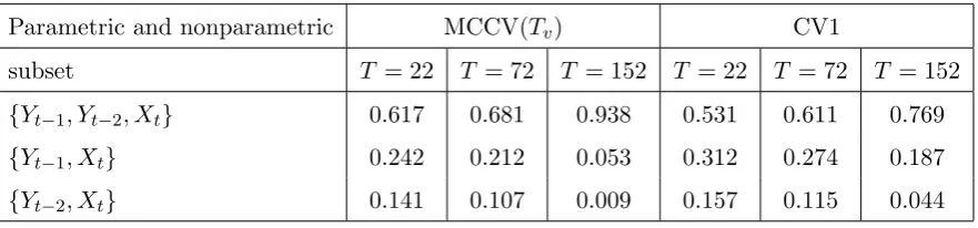
Table 3.2. The parametric MCCV(Tv) and CV1 based probabilities for Example 3.1
Parametric and nonparametric MCCV(Tv) CV1
subset T = 22 T = 72 T = 152 T = 22 T = 72 T = 152
{Yt−1, Yt−2, Xt} 0.617 0.681 0.938 0.531 0.611 0.769
{Yt−1, Xt} 0.242 0.212 0.053 0.312 0.274 0.187 {Yt−2, Xt} 0.141 0.107 0.009 0.157 0.115 0.044
Remark 3.1. (i) First, Tables 3.1 and 3.2 show that both the CV1 function and
the MCCV(Tv) function can be implemented in practice. Second, Table 3.1 supports the
validity of our definition of optimum subset (see Assumption 2.1). Third, the detailed simulation results show that ˆD0 is a reasonably good estimator of D0 even when the sample sizeT is as small as 22 as shown in Table 3.1. Fourth, Table 3.2 shows that both the MCCV(Tv) function and the CV1 function can identify the optimum parametric
regressor {Yt−1, Yt−2}. Finally, the performance of the MCCV(Tv) is better than the
CV1: this is a reflection of the fact that MCCV(Tv) leads to a consistent subset selection
while CV1 does not.
[image:21.595.92.533.452.555.2]the ASE value for the true model (see the fifth row and sixth column) is 0.0051 and smaller than 0.0054, the ASE for the second best model (see the eighth row and sixth column). For the same model, the ASE decreses whenT increases. For example, when
T = 152, the ASE for the true model (see the fifth row and eighth column) is already as small as 0.0010.
(iii) Before using the standard normal kernel function k(·), we also calculated the corresponding probabilities and ASEs for a uniform kernel function. Our computation shows that the small sample results for the standard normal kernel function are much better and more stable than those for the uniform kernel. In the meantime, besides the bandwidth interval HT, we also calculated the CV1 function over all possible intervals.
Our computation indicates thatHT is the smallest possible interval, on which the CV1
function for each possible model can attain the smallest value.
(iv) Throughout Example 3.1, we point out that Assumptions 2.1 and A.1–A.5 are satisfied. In theory, Assumption A.5(i) is a very minimal model identifiability condition. In practice, it is not easy to justify the model identifiability condition. For Example 3.1, however, we have been able to calculate the quadratic form explicitly and to show that the quadratic form is positive with probability one.
We now compare our semiparametric model selection function CV1 with the fully nonparametric model selection function. For the same Example 3.1, consider the case whereYt−1,Yt−2,XtandXt−1are selected as the candidates of nonparametric regressors. For an application of the CV1 function, we choose the samew,k andhdefined as above, and define forj = 2,3,4
Kj(u1, u2, . . . , uj) = j
Y
i=1
k(uj)
for the multivariate kernel function involved inWD(−t)(t, s) and WD(t, s).
LetXtD1 = (Yt−1, Yt−2, Xt, Xt−1)
τ,X
tD2 = (Yt−1, Yt−2, Xt)
τ,X
tD3 = (Yt−1, Yt−2, Xt−1)
τ,
XtD4 = (Yt−1, Xt, Xt−1)
τ,X
tD5 = (Yt−2, Xt, Xt−1)
τ,X
tD6 = (Yt−1, Yt−2)
τ,X
tD7 = (Yt−1, Xt)
τ,
XtD8 = (Yt−1, Xt−1)
τ, X
tD9 = (Yt−2, Xt)
τ, X
tD10 = (Yt−2, Xt−1)
τ, X
tD11 = (Xt, Xt−1)
τ,
XtD12 = Yt−1, XtD13 = Yt−2, XtD14 = Xt−1, and XtD15 = Xt. Then |D1| = 4, |D2| =
|D3| = |D4| = |D5| = 3, |D6| = |D7| = |D8| = |D9| = |D10| = |D11| = 2, and
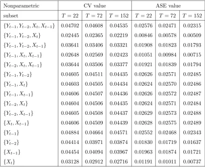
correspond-ing CV1 values. For each of the three sample sizes T = 22, 72 and 152, we calculated CV1 value and the sample average squared error (ASE). Table 3.3 below provides the CV1 values and the corresponding ASE values for the nonparametric model selection.
Table 3.3. The nonparametric CV1 based minimum CV values and ASEs for Example 3.1
Nonparametric CV value ASE value
subset T = 22 T = 72 T = 152 T = 22 T = 72 T = 152
{Yt−1, Yt−2, Xt, Xt−1} 0.04702 0.04608 0.04535 0.02576 0.02471 0.02315 {Yt−1, Yt−2, Xt} 0.02445 0.02365 0.02219 0.00846 0.00578 0.00509 {Yt−1, Yt−2, Xt−1} 0.03641 0.03406 0.03321 0.01908 0.01823 0.01793
{Yt−1, Xt, Xt−1} 0.02648 0.02569 0.02423 0.01051 0.00984 0.00715
{Yt−2, Xt, Xt−1} 0.03644 0.03506 0.03377 0.01921 0.01839 0.01794
{Yt−1, Yt−2} 0.04605 0.04511 0.04435 0.02626 0.02571 0.02485
{Yt−1, Xt} 0.04603 0.04505 0.04434 0.02624 0.02570 0.02486
{Yt−1, Xt−1} 0.04606 0.04507 0.04436 0.02626 0.02572 0.02487
{Yt−2, Xt} 0.04604 0.04506 0.04435 0.02624 0.02571 0.02484
{Yt−2, Xt−1} 0.04605 0.04508 0.04437 0.02629 0.02573 0.02488
{Xt, Xt−1} 0.04606 0.04509 0.04439 0.02628 0.02575 0.02489
{Yt−1} 0.04884 0.04664 0.04571 0.02552 0.02468 0.02343
{Yt−2} 0.04414 0.03971 0.03874 0.01830 0.01719 0.01637
{Xt−1} 0.04454 0.04094 0.03967 0.01963 0.01874 0.01721
{Xt} 0.03128 0.02912 0.02716 0.01191 0.01011 0.00737
Remark 3.2. First, Table 3.3 shows that the true subset {Yt−1, Yt−2, Xt} is readily
for Tables 3.1 and 3.3, we know that the computation of the semiparametric model selec-tion funcselec-tion CV1 is much less expensive than that of the nonparametric model selecselec-tion function. Therefore we conclude that when selecting an optimum subset of nonparamet-ric regressors for a partially linear model, the semiparametnonparamet-ric model selection function CV1 is much more efficient than the usual nonparametric model selection function.
Example 3.2. Fisheries Western Australia (WA) manages commercial fishing in
Western Australia. Simple Catch and Effort statistics are often used in regulating the amount of fish that can be caught and the number of boats that are licensed to catch them. The establishment of the relationship between the Catch (in kilograms) and Effort (the number of days the fishing vessels spent at sea) is very important both commerically and ecologically. This example considers using the proposed model selection procedure to find a best possible model for the relationship between catch and effort.
The historical monthly fishing data from January 1976 through to December 1999 available to us comes from the Fisheries WA Catch and Effort Statistics (CAES) data-base. Existing studies from the Fisheries suggest that the relationship between the catch and the effort does not look like linear while the dependence of the current catch on the past catch appears to be linear. This suggests using a partially linear model of the form
Ct=β1Ct−1+. . .+βpCt−p+φ(Et, Et−1, . . . , Et−q+1) +ǫt,
where ǫt is a random error, Ct and Et represent the catch and the effort at time t,
respectively. In the detailed computation, we use the transformed data Yt = log10(Ct)
and Xt = log10(Et) satisfying the following model
Yt+r =β1Yt+r−1+. . .+βpYt+r−p+φ(Xt+r, . . . , Xt+r−q+1) +et, (3.1)
wherer = max(p, q) and et is a random error with zero mean and finite variance.
Before using model (3.1), we need to choose an optimum and compact form of model (3.1). We consider the case of p = 4 and q = 5 and then find an optimum model. For this case, there are 24−1 = 15 different parametric regressors and 25−1 = 31 different nonparametric regressors for model (3.1).
Similar to Example 3.1, we define the parametric candidates UtAi for 1≤i≤15 and
the nonparametric candidates XtDj for 1≤j ≤31. It follows that
whereβAi and φDj are similar to those ofβA and φD, and each etij is assumed to be an
i.i.d. random error with zero mean and finite variance.
For this case, we consider usingK4(u1, . . . , uj) =Qji=1k(ui) forj = 1,2,· · ·,5 for the
multivariate kernel function involved inWD(−t)(t, s) andWD(t, s). We use the same w(·), k(·) and HT as in Example 3.1.
First, we use the first 144 observations of the data from January 1976 to December 1987 for the selection of a best possible partially linear model. In the detailed calculation of the MCCV(Tv) function, we choose b=T = 144,Tc = [T3/4] = 41 andTv =T −Tc =
103. The semiparametric CV1 and parametric MCCV(Tv) values for model (3.2) are
calculated. The combined semiparametric CV1 and parametric MCCV(Tv) selection
procedure then suggests using the following partially linear prediction model
Yt+5 = ˆβYt+4+ ˆφ(Xt+5, Xt+3), 1≤t≤144, (3.3)
where ˆβ = 0.2098 and ˆφ(·,·) is as defined before. The optimum value for the bandwidth involved in (3.3) is ˆh1 = 0.080088.
We also consider using the nonparametric CV selection function for the same part of the data for the case where Yt+i for 1 ≤ i ≤ 4 and Xt+j for 1 ≤ j ≤ 5 are candidates
of nonparametric regressors. The nonparametric CV selection function suggests the following nonparametric prediction model
Yt+5 = ˆm(Yt+4, Xt+5, Xt+3), 1≤t≤144, (3.4)
where ˆm(·,·,·) is the usual nonparametric regression estimator as defined before. The optimum value for the bandwidth involved in (3.4) is ˆh2 = 0.08011.
When we assume that the dependence of Yt+5 on Yt+i for 1 ≤ i ≤ 4 and Xt+j for
1≤j ≤5 is linear, the conventional AIC criterion suggests the following linear prediction model for the first part of the data
Yt+5 = ˆβ1Yt+4+ ˆβ2Xt+5+ ˆβ3Xt+3, 1≤t≤144, (3.5)
where ˆβ1 = 0.4944, ˆβ2 = 0.8740 and ˆβ3 =−0.1923.
selected models. For the whole data set, the estimated error variances for the partially linear model (3.3), the fully nonparametric model (3.4) and the completely linear model (3.5) were 0.00935, 0.01508 and 0.02661, respectively.
Remark 3.4. Example 3.2 shows that if a partially linear model among the possible
partially linear models is an appropriate model for the data, then the combined semipara-metric CV1 and MCCV(Tv) selection procedure is capable of finding it. Furthermore,
when using both the nonparametric CV1 selection criterion and a parametric AIC se-lection criterion to check whether the partially linear model (3.3) is the best possible model, both the nonparametric and parametric selection criteria support the selection of the regressors. In addition, the estimated error variance for the partially linear model is the smallest one among the partially linear model (3.3), the nonparametric regression model (3.4) and the parametric linear model (3.5). Our findings in Example 3.2 are consistent with existing studies from the Fisheries in that the relationship between the catch and the effort appears to be nonlinear while the current catch depends linearly on the past catch.
Remark 3.5. As expected, there is no evidence of conditional heteroscedasticity in
the catch–effort data. In both theory and practice, however, we need to consider the heteroscedastic case. As the homoskedasticity assumption given in Assumption A.1 is a convenient but not vital condition, we can relax it and obtain similar model selection functions and the corresponding consistency results of Theorems 2.1–2.2, but the proofs of Theorems 2.1–2.2 would be extremely technical.
Remark 3.6. This paper only considers using the Nadaraya-Watson (NW) kernel
that the LPK estimation method is superior to the GM estimation method.
4. Discussion
In recent years, there have been growing interests in applying iterative algorithms in nonparametric and semiparametric smoothing. However, such techniques cannot provide a ’model’ whose value can be calculated at a new design point with the same convenience as in linear models. Before selecting a fully nonparametric time series model for a given set of data, our research suggests using the computer-intensive semiparametric time series model selection to determine whether a partially linear time series model is more appropriate than the fully nonparametric time series model for the given set of data, as semiparametric methods can provide a ’model’ with better predictive power than is available from nonparametric methods (see Example 3.2).
We acknowledge the computing expenses of the CV based selection procedure. In our detailed simulation and computing for Examples 3.1 and 3.2, we have used some optimal algorithms, such as some vectorised algorithms in the calculation of the CV1 function and the MCCV function of many possible candidates. The final computing time for each example is reasonable. We have not tried the backward or forward selection suggested by Shao (1993), although we think it might be less expensive in terms of computing time. We think that further discussion of computing algorithms is beyond the scope of this paper.
APPENDIX A
Throughout Appendices A–C, let C (C <∞) denote a positive constant which may have
different values at each appearance.
Assumption A.1. Assume that the stochastic process (Yt, Ut, Xt) is strictly stationary and α–mixing with the mixing coefficient α(T) = CηT, where 0 < C < ∞ and 0 < η < 1 are constants. In addition, et = Yt−E[Yt|Ut, Xt] is a stationary martingale difference with respect to Ωt =σ{(Ys, Us+1, Xs+1) : 1≤s≤t−1}, which is a sequence of σ-fields generated
by {(Ys, Us+1, Xs+1) : 1≤ s ≤t−1}. Suppose that P E[e2t|Ωt] =σ20
= 1, where 0 < σ02 =
Assumption A.2. For every D ∈ D, KD is a |D|–dimensional symmetric, Lipschitz con-tinuous probability kernel function with R
||u||2KD(u)du < ∞, and KD has an absolutely integrable Fourier transform, where|| · || denotes the Euclidean norm.
Assumption A.3. LetSwbe a compact subset ofRq andwbe a weight function supported onSwandw≤Cfor some constantC. For everyD∈ D, letRX,D⊆R|D|= (−∞,∞)|D|be the
subset such thatXtD ∈RX,DandSD be the projection ofSωinRX,D(that is,SD =RX,D∩Sω). Assume that the marginal density function, fD(·), of XtD, and all the first two derivatives of
fD(·), φ1(·) and φA,D(·), are continuous on RX,D, and on SD the density function fD(·) is bounded below byCD and above by CD−1 for someCD >0, where φ1(x) =E[Yt|XtD=x] and
φA,D(x) =E[UtA|XtD=x] for everyA∈ Aand D∈ D.
Assumption A.4. There exist absolute constants 0< C1 <∞ and 0< C2 <∞ such that
for any integerl≥1
sup
x A∈Asup,D∈D
En|Yt−E[Yt|(UtA, XtD)]|l|XtD =x
o
≤C1and sup
x A∈Asup,D∈D
En||UtA||l|XtD =x
o
≤C2.
Assumption A.5. (i) For ηtA and ηt defined in (2.11), let ηA = (η1A, . . . , ηT A)τ and
η= (η1, . . . , ηT)τ. Assume that when MAis in Category I,
lim inf T→∞
1
T(ηβ)
τ I
T −ηA(ηAτηA)+ητA
ηβ >0 in probability.
(ii) AsT → ∞,
Tv
T →1, Tc =T−Tv → ∞ and T2 T2
cb → 0.
Remark A.1. Assumptions A.1–A.4 are standard in this kind of problem. See (A.1) of Cheng and Tong (1993). Due to Assumption A.3, we do not need to assume that the
marginal density of Xt has a compact support. Assumptions A.2–A.4 are a set of extensions of some existing conditions to the α–mixing time series case. See for example, (A)–(E) of Zhang (1991), (A2)–(A5) of Cheng and Tong (1993), and (C.2)–(C.5) of Vieu (1994). As
pointed out in Remark 2.4(ii), when Xt and Ut are independent, Assumption A.5(i) imposes only an asymptotic and minimal model identifiability condition on the linear component. This
means that Assumption A.5(i) is a natural extension of condition (2.5) of Shao (1993) to the semiparametric time series setting. Assumption A.5(ii) corresponds to conditions (3.12) and
APPENDIX B
In this appendix, we provide a detailed proof for Theorem 2.1.The following lemmas are required to prove Theorem 2.1.
Lemma B.1. Under the conditions of Theorem 2.1, we have for everyD∈ D
CV1(D, h) = 1
T
T
X
t=1
e2tD0w(Xt) +V(D, h) +op(V(D, h)),
where for everyD∈ D1 and h∈HT D
V(D, h) =a1(D, h)
1
T h|D|+a2(D, h)h
4+o
p(V(D, h)),
in which a1(D, h) and a2(D, h) are positive constants depending only on (D, h), and for every
D∈ D, D6∈ D1, and h∈HT D
V(D, h) =En[Utτ(β(D)−β(D0)) +φD(XtD)−φD0(XtD0)]2w(Xt)o+op(1).
Then, we have
CV1(D) = inf h∈HT D
CV1(D, h) = 1
T
T
X
t=1
e2tD0w(Xt) +R(D) +op(1),
where etD0 is as defined in (2.4), for D∈ D1
R(D) =CDT−
4 4+|D| +o
p(T−
4 4+|D|),
where CD is a positive constant depending only on D, and for D∈ D butD6∈ D1,
R(D) =En[Utτ(β(D)−β(D0)) +φD(XtD)−φD0(XtD0)]
2w(X
t)
o
+op(1).
The following lemmas are needed to complete the proof of Lemma B.1.
Lemma B.2. Under the conditions of Theorem 2.1, we have
δ(D, h)( ˆβ(D, h)−β(D)) =op(1) (B.1)
uniformly overD∈ D and h∈HT D, where δ(D, h) = max{(T h|D|)1/2, h−2}. Proof. It follows from (2.7) that
ˆ
β(D, h)−β(D) = ( ˜Σ(D, h))+ T
X
t=1
˜
+( ˜Σ(D, h))+ T
X
t=1
˜
Ut(D, h)( ˆφ2t(XtD, h)−φ2(XtD))τβ(D)+( ˜Σ(D, h))+ T
X
t=1
˜
Ut(D, h)(φ1(XtD)−φˆ1t(XtD, h)).
In order to prove (B.1), it suffices to show that asT → ∞
√
T∆D
ˆ
β(D, h)−E[ ˆβ(D, h)]→N(0, E[e2tDξtDξtDτ ])
and
E[ ˆβ(D, h)]−β(D) =O(h4) +O(h2(T h|D|)−1/2) =o(δ(D, h)−1), (B.2)
whereξtD =Ut−E[Ut|XtD] and ∆D =E[ξtDξτtD] is as defined in Assumption 2.1(i).
In order to prove (B.2), it suffices to show that
1
TΣ(˜ D, h) =
1 T T X t=1 ˜
Ut(D, h) ˜Ut(D, h)τ →p∆D, (B.3)
1 √ T T X t=1
ξtDetD →N(0, E[etD2 ξtDξtDτ ]), (B.4)
1
T
T
X
t=1
(φ1(XtD)−φˆ1t(XtD, h))2=op(δ(D, h)−1), (B.5)
1
T
T
X
t=1
(φ2(XtD)−φˆ2t(XtD, h))(φ2(XtD)−φˆ2t(XtD, h))τ =op(δ(D, h)−1), (B.6)
1
T
T
X
t=1
(φ2(XtD)−φˆ2t(XtD, h))rtD =op(δ(D, h)−1), (B.7)
1
T
T
X
t=1
(φ1(XtD)−φˆ1t(XtD, h))ξtD =op(δ(D, h)−1), (B.8)
wherertD =etD orξτtD and ∆D are as defined above.
The proofs of (B.5)–(B.8) are standard. The details are similar to Lemma A.2(ii) of Gao and Yee (2000). In the proof of (B.5)–(B.8), Proposition 14.1 of Cheng and Tong (1993) is
used repeatedly. Using Assumptions A.1 and A.4 and applying the fact that E[ξtDetD] =
E{ξtDE[etD|(Ut, XtD)]} = 0, we can prove (B.4) by applying the classical martingale limit theorem (see Lemma 3.3 of Gao and Liang 1995 for example). The proof of (B.3) follows from
Assumption A.4, (B.6), (B.7), the Cauchy-Schwarz inequality and
1 T T X t=1 ˜
Ut(D, h) ˜Ut(D, h)τ = 1
T
T
X
t=1
ξtDξtDτ +1
T
T
X
t=1
+1
T
T
X
t=1
(φ2(XtD)−φˆ2t(XtD, h))ξtDτ + 1
T
T
X
t=1
ξtD(φ2(XtD)−φˆ2t(XtD, h))τ.
The first term then converges to ∆D in probability and the other terms converge to zero in
probability due to the use of some convergence results of nonparametric estimates (see Robinson 1983 for example).
Lemma B.3. (i) Under the conditions of Theorem 2.1, we have for every given D ∈ D1
andh∈HT D
V1(D, h) =
1 T T X t=1 n
φ1(XtD)−φˆ1t(XtD, h)
o2
w(Xt) =d1(D, h)
1
T h|D|+d2(D, h)h
4+o
p{V1(D, h)},
(B.9)
V2(D, h) =
1 T T X t=1
φ2(XtD)−φˆ2t(XtD, h) φ2(XtD)−φˆ2t(XtD, h)
τ
w(Xt)
=d3(D, h) 1
T h|D| +d4(D, h)h
4+o
p{V2(D, h)}, (B.10)
where {di(D, h) : 1 ≤ i ≤ 2} are positive constants and {dj(D, h) : 3 ≤ j ≤ 4} are positive
definite matrices.
(ii) Under the conditions of Theorem 2.1, we have for every given D ∈ D, D 6∈ D1 and
h∈HT D
V1(D, h) =E
n
[φ1(XtD)−φ1(XtD0)]
2w(X
t)
o
+op(1), (B.11)
V2(D, h) =E{(φ2(XtD)−φ2(XtD0)) (φ2(XtD)−φ2(XtD0))
τw(X
t)}+op(1). (B.12)
Proof. We prove only (B.9) and (B.11) and the others follow similarly. In order to prove (B.9) and (B.11), it suffices to show that forD∈ D1 and h∈HT D
¯
V1(D, h) =
1 T T X t=1 n ˆ
φ1(XtD, h)−φ1(XtD)
o2
w(Xt) =d1(D, h)
1
T h|D|+d2(D, h)h
4+o
p( ¯V1(D, h)),
(B.13)
and forD6∈ D1 andh∈HT D
¯
V1(D, h) =E
n
[φ1(XtD)−φ1(XtD0)]
2w(X
t)
o
+op(1) (B.14)
and
sup D∈D
sup h∈HT D
|V¯1(D, h)−V1(D, h)|
¯
V1(D, h)
=op(1), (B.15)
Similar to the proofs of Lemmas 14.7 and 14.4 of Cheng and Tong (1993), equations (B.13)–
(B.15) can be proved. Similar lemmas for the i.i.d. case and the time series case can be found in equations (5.3) and (5.4) of Vieu (1994), and Lemmas 2 and 8 of H¨ardle and Vieu (1992),
respectively.
Lemma B.4. Under the conditions of Theorem 2.1, we have
V(D, h) = 1
T
T
X
t=1
nh
Utτβˆ(D, h) + ˆφt(XtD,βˆ(D, h))
i
−[Utτβ(D0) +φD0(XtD0)]
o2
w(Xt)
=d5(D, h)
1
T h|D| +d6(D, h)h
4+o
p(V(D, h)) (B.16)
for everyD∈ D1 andh∈HT D, and
V(D, h) =En[Utτ(β(D)−β(D0)) +φD(XtD)−φD0(XtD0)]
2w
(Xt)
o
+op(1) (B.17)
for every D∈ D, D 6∈ D1 and h ∈ HT D, where d5(D, h) and d6(D, h) are positive constants
only depending on (D, h).
Proof. Obviously,
V(D, h) = 1
T
T
X
t=1
n
Utτβˆ(D, h)−β(D0)
o2
w(Xt)+ 1
T
T
X
t=1
n
ˆ
φt(XtD,βˆ(D, h))−φD0(XtD0)
o2
w(Xt)
+2
T
T
X
t=1
n
Utτβˆ(D, h)−β(D0)
o n
ˆ
φt(XtD,βˆ(D, h))−φD0(XtD0)
o
w(Xt)
≡V(D, h)1+V(D, h)2+V(D, h)3, (B.18)
where the symbol ”≡” indicates that the terms of the left-hand side are represented by those of the right-hand side correspondingly.
Similar to the proof of Lemmas B.2 and B.3, we have for every D∈ D1 and h∈HT D
V(D, h)2=V1(D, h) +β(D)τV2(D, h)β(D) +op(V(D, h)2), (B.19)
and
sup D∈D
sup h∈HT D
V(D, h)1
V(D, h)2
=op(1), sup D∈D
sup h∈HT D
V(D, h)3
V(D, h)2
=op(1). (B.20)
On the other hand, using Lemmas B.2 and B.3 again, we have for every D∈ D, D6∈ D1
andh∈HT D
Therefore, equations (B.18)–(B.21) complete the proof of (B.16) and (B.17).
Proof of Lemma B.1. It follows from the definition of CV1(D, h) that
CV1(D, h) = 1
T
T
X
t=1
n
Yt−Utτβˆ(D, h)−φˆt(XtD,βˆ(D, h))
o2
w(Xt)
≡ T1 T
X
t=1
e2tD0w(Xt) +V(D, h) +R(D, h), (B.22)
whereR(D, h) = T2 PT
t=1
n
Utτβ(D0)−βˆ(D, h)
+φD0(XtD0)−φˆt(XtD,αˆ(D, h))
o
etD0w(Xt).
Analogous to the proof of (14.25) of Cheng and Tong (1993) (see also (A.25) of Gao and Yee 2000), we have
sup D∈D
sup h∈HT D
|R(D, h)|
V(D, h) =op(1). (B.23)
Thus, equations (B.22) and (B.23) imply for every D∈ D and h∈HT D
CV1(D, h) = 1
T
T
X
t=1
e2tD0w(Xt) +V(D, h) +op(V(D, h)). (B.24)
Therefore, Lemma B.4 and equation (B.24) imply Lemma B.1.
Proof of Theorem 2.1. Since equation (B.24) holds for every D ∈ D, we have that there exists ¯hD ∈HT D such that
CV1(D,¯hD) = inf h∈HT D
CV1(D, h)
and
CV1(D) = CV1(D,¯hD) = inf h∈HT D
CV1(D, h) = 1
T
T
X
t=1
e2tD0w(Xt) +CDT−
4 4+|D| +o
p
T−4+|4D|
(B.25)
for everyD∈ D1, whereCD is a positive constant possibly depending onD.
Using the fact that Assumption 2.1 implies|D|>|D0|for everyD∈ D1, by (B.25) we have
asT → ∞
P(CV1(D)>CV1(D0)) =P
T4+|4D0|(CV1(D)−CV1(D
0))>0
=P
CDT
4(|D|−|D0|) (4+|D|)(4+|D0|) −C
D0 +op
T
4(|D|−|D0|) (4+|D|)(4+|D0|)
>0
→1. (B.26)
On the other hand, for every D ∈ D but D 6∈ D1, we obtain by (B.24) and (B.17) that there exists a positive constantπ(D, D0) depending only on (D, D0) such that
in probability asT → ∞.
Each of (B.26) and (B.27) implies
lim
T→∞P( ˆD0 =D0) = 1. (B.28)
Furthermore, similar to the proof of (2.3) of H¨ardle, Hall and Marron (1988), using equa-tions (B.25) and (B.28) we can show that asT → ∞
ˆ
h h0 →p
1,
where ˆh= ¯hDˆ0 and h0=CD0T
− 1 4+|D0|.
The proof of Theorem 2.1 is finally completed.
Proof of Corollary 2.1. It is a special case of Theorem 2.1.
Proof of Corollary 2.2. The proof is similar to the proofs of Lemmas B.1 and B.4.
Proof of Theorem 2.2. In view of the proofs of Theorems 1 and 2 of Shao (1993), in order to prove Theorem 2.2, it suffices to show that conditions (3.3) and (3.4) of Shao (1993) hold
in probability with respect to the probability measure of (Yt, Ut, Xt) and that condition (3.21) of Shao (1993) holds in probability with respect to both the probability measure of (Yt, Ut, Xt) and the random selection of R. Condition (2.5) of Shao (1993) now corresponds to condition
(2.16) for our case. In other words, we need to prove (2.16) and the following conditions:
max S∈R
1
Tv
X
t∈S
VtVtτ− 1
Tc
X
t∈Sc
VtVtτ
=op(1), (B.29)
VτV =Op(T) and (VτV)−1=Op(T−1), (B.30)
lim
T→∞maxt≤T ptA= 0 for any A∈ A, (B.31) whereptA is the tth diagonal element of the projection matrix PA defined in (2.14).
The proofs of (2.16) and (B.29)–(B.31) are relegated to Appendix C below. In view of the
conditions of Theorem 2.2, we modify some parts of the proofs of Theorems 1 and 2 of Shao (1993). For example,nc,nv,nand the termo nncinvolved in the proofs of Theorems 1 and 2 of Shao (1993) need to be replaced byTc,Tv,T andop
Tc
T
respectively. Some notational changes