http://dx.doi.org/10.4236/ijcns.2014.78032
How to cite this paper: Jiao, C.W., Gao, S.X., Yang, W.G., Xia, Y.B. and Zhu, M.M. (2014) A Fast Heuristic Algorithm for Mi-nimizing Congestion in the MPLS Networks. Int. J. Communications, Network and System Sciences, 7, 294-302.
http://dx.doi.org/10.4236/ijcns.2014.78032
A Fast Heuristic Algorithm for Minimizing
Congestion in the MPLS Networks
Chengwen Jiao
1, Suixiang Gao
1, Wenguo Yang
1*, Yinben Xia
2, Mingming Zhu
21School of Mathematical Sciences, University of Chinese Academy of Sciences, Beijing, China 2Huawei Technologies Co. Ltd., Beijing, China
Email: [email protected],*[email protected]
Received 4 July 2014; revised 25 July 2014; accepted 5 August 2014
Copyright © 2014 by authors and Scientific Research Publishing Inc.
This work is licensed under the Creative Commons Attribution International License (CC BY).
http://creativecommons.org/licenses/by/4.0/
Abstract
In the multiple protocol label-switched (MPLS) networks, the commodities are transmitted by the label-switched paths (LSPs). For the sake of reducing the total cost and strengthening the central management, the MPLS networks restrict the number of paths that a commodity can use, for maintaining the quality of service (QoS) of the users, the demand of each commodity must be sa-tisfied. Under the above conditions, some links in the network may be too much loaded, affecting
the performance of the whole network drastically. For this problem, in [1], we proposed two
ma-thematical models to describe it and a heuristic algorithm which quickly finds transmitting paths for each commodity are also presented. In this paper, we propose a new heuristic algorithm which finds a feasible path set for each commodity, and then select some paths from the path set through a mixed integer linear programming to transmit the demand of each commodity. This strategy reduces the scale of the original problem to a large extent. We test 50 instances and the results show the effectiveness of the new heuristic algorithm.
Keywords
MPLS-Network, k-Splittable Flow, Minimum Congestion, Heuristic Algorithm
1. Introduction
In the modern broadband communication networks, namely the multiple protocol label-switched networks (MPLS), data packets are transmitted through the label-switched paths (LSPs). An important feature of MPLS is its ability to set up traffic engineering mechanism (MPLS-TE). It can control the structure of the traffic for each customer by setting restrictions on the number of routes the customer used. In order to preserve the QoS
quirement, the demand of each customer must be satisfied. Using a single path would possibly increase the con-gestion of the network, while, on the other hand, a huge number of LSPs would decrease the performance of the protocol, and the intermediate situation is considered in the MPLS network. When limiting the number of sup-porting LSPs, we should try to minimize the congestion of the network under the condition that all data are transmitted.
This problem can be described formal as follows: Given a directed graph G=
(
V E,)
, which denotes the MPLS network, Vertex set V and edge set E denote the nodes and the links of the network, respectively. Each edge e∈E has a positive capacity ue, denoting the bandwidth of the corresponding link in the network. A set of commodities is denoted by L, each commodity l∈L has a source node sl, a destination node tl, an amount dl to be delivered and a maximal number of directed paths that the commodity can use kl. Limit-ing the number of paths that a commodity can use is in fact the k-splittable multi-commodity flow problem which is introduced by Baier [2]. When kl =1 for all l∈L, the problem collapses to the multi-commodity unsplittable flow problem, and whenkl ≥ E for all l∈L, the problem is an ordinary multi-commodity flow problem. In this paper, we focus on minimizing congestion of the MPLS network under the condition thatl
k < E for all l∈L.
Kleinberg [3] introduced several optimization versions of the unsplittable flow problem. In the “minimum congestion” version, the task is to find the smallest value
λ
>0 such that there exists an unsplittable flow that uses at most aλ
-fraction of the capacity of any edge. The “minimum number of rounds” version asks for a partition the set of commodities into a minimum numberof subsets (rounds) and a feasible unsplittable flow for each subset. The “maximum routable demands” problem is to find a feasible unsplittable flow for a subset of demands maximizing the sum of demands in the subset.As for the k-splittable flow problem, researchers generalize the above optimization versions and there is a lot of study on the related problems. Baier et al. [2], who solved the Maximum Budget-Constrained Singe- and Multi-commodity k-splittable flow problem using approximationalgorithms. The authors proved that the maxi-mum single-commodity k-splittable flow problem is NP-hard in the strong sense for directedgraphs.Koch et al. [4] proved that the maximum multi-commodity flow problem was NP-hard in the strong sense for directed as well
as undirected graphs,and showed that when P≠NP, the best possible approximation factor is 5
6. Kollipoul- ous [5] considered the single-source Minimum Cost 2-splittable flow problem with budget constraints and with the assumption thatthe minimum edge capacity was larger than the maximum commodity demand. The author presented an approximation algorithm with factor (2, 1)for minimum congestion and cost. The result was gene-ralized to the k-splittable problem by Salazar and Skutella [6] with a resulting approximation factor of
(
1 1 1 ,1)
2 1
k k
+ +
− .
References [7]-[11] are part of the researches solving the related single- and multi-commodity k-splittable flow problems exactly. The authors design algorithms that are based on branch-and-price strategy. Branch-and- price is usually used to solve large scale mixed integer linear programs. It combines column generation and branching strategies. In spite of this, the running time of the branch-and-price algorithm cannot obtain exact so-lutions in short time, and is not suitable for the high speed networks.
In the MPLS networks, the number of paths that a commodity can use is limited due to the reduction of the total cost, and we need to satisfy all demands of the commodities in a relative low congestion network. We aim to minimize the congestion as much as possible. Since this problem is NP-hardand obtaining exact solutions is impossible in short time, we must arrange the data on some paths quickly, hence the fast and good heuristic al-gorithms are badly needed. In this paper, we consider a special case that all the commodities in L have a common source node.
The main contribution of this paper is as follows: for the single-source multi-commodity k-splittable flow problem, we propose a new heuristic algorithm, different from the old algorithm that is proposed in [1]. The new algorithm reduces the original problem to a small scale of mixed-integer linear programming. And in the last section, we test 50 instances, and the performance of the new algorithm outperforms the old one.
2. Problem Description and Mathematical Models
We describe the problem in a more general case. In the minimum congestion k-splittable multi-commodity flow problem, a directed graph G=
(
V E u, ,)
is given with V =n and E =m, with arc capacities ue >0,e E
∀ ∈ . A set of commodities is denoted by L, each commodity l∈L has a certain amount of demand dl
to transmit, a source node sl and a destination node tl, and the number of paths that commodity l can use l
k . The goal is to find a flow f that satisfies all demands of the commodities and minimize the congestion: Find the smallest
α
such that there exists a feasible flow satisfying the demands and the path restrictions if all capacities are multiplied byα
. In [1], we first propose two different mathematical models, namely the arc-path and arc-flow model. In this paper, we also use the two models to describe our problem.2.1. The Arc-Path Model
Let Pl denotes the set of all paths of commodity l, xlp denotes the flow value on path p∈Pl of commod-ityl, l
{ }
0,1p
y ∈ denoting whether or not path p∈Pl is used by commodity
l. up: min=
{
ue:e∈p}
de-notes the maximum flow value that path p can transmit.This problem is formulated as follows:
min
α
. .
l
p l
e p e
l L p P
s t δ x α u e E
∈ ∈
≤ ⋅ ∀ ∈
∑ ∑
(1)
l
l
p l
p P
x d l L
∈
= ∀ ∈
∑
(2)xlp≤ylp⋅M u⋅ p ∀ ∈l L, ∀ ∈p Pl (3)
l
l l
p p P
y k l L
∈
≤ ∀ ∈
∑
(4)l 0 , l p
x ≥ ∀ ∈l L ∀ ∈p P (5)
{ }
ylp∈ 0,1 ∀ ∈l L, ∀ ∈p Pl (6)
α
>0, (7)The objective function is to minimize the factor that each edge can multiply. The first constraints (1) ensure that the flow value on an edge e is at most
α
of its capacity,δ
ep∈{ }
0,1 is a constant, if e∈p, 1p e δ = , otherwise δep =0. The constraints (2) ensure that each commodity's demand is satisfied, and constraints (3) in-dicate that only path p is used by commodity l, that is ylp=1, the flow value
l p
x can be non-negative. The notation M is any upper bound of the objective value, which can be selected by l min
l L∈ d u
∑
with{
}
min min e:
u = u e∈E . Constraints (4) limit the number of paths that a commodity can use. Constraints (5)-(7) force the variables to take on feasible values.
2.2. The Arc-Flow Model
The variable hl e
x refers to the flow value of the h -th path of commodity l∈L on edge e∈E , 1, 2, , l
h= k , and binary variable hl e
y denotes whether or not edge e is used by the h-th path of commodity
l. We use A+
( )
v and A−( )
v to denote the outgoing arcs and ingoing arcs of node v∈V , respectively. Then the arc-flow model is stated as follows:min
α
( ) ( ) 1 , . . l l l k hl hl
e e l
h e A s e A s
st x x d l L
+ − = ∈ ∈ − = ∀ ∈
∑ ∑
∑
(8)1 , l k hl e e
l L h
x α u e E
∈ =
≤ ⋅ ∀ ∈
∑∑
(9)( ) ( )
{ }
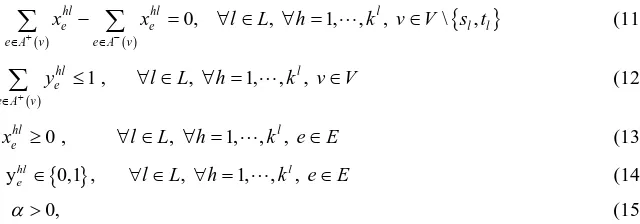
ehl ehl 0, , 1, , l, \ l,l
e A v e A v
x x l L h k v V s t
+ −
∈ ∈
− = ∀ ∈ ∀ = ∈
∑
∑
(11)( )
hl 1 , , 1, , l, e
e A v
y l L h k v V
+
∈
≤ ∀ ∈ ∀ = ∈
∑
(12)xehl ≥0 , ∀ ∈l L, ∀ =h 1,,kl, e∈E (13)
{ }
yehl∈ 0,1 , ∀ ∈l L, ∀ =h 1,,kl, e∈E (14)
α
>0, (15)Constraints (8) ensure that each commodity’s demand is satisfied, and constraints (9) ensure the flow on each edge is at most
α
times of its capacity, constraints (10) indicate that only if edge e is used by the h-th path of commodity l can the variable xehl be positive. Constraints (11) are the flow conservation constraints and (12) are used to prevent cycles connecting to the h-th path of commodity l for each l∈L, h=1,,kl. Constraints (13)-(15) force the variables to take on feasible values.The main difference of the two mathematical models is that in the arc-path model each commodity has a feasible path set which contains all the paths for the commodity in the network and we only need to select some paths from the path set to transmit the demand. Sometimes, determining all the feasible paths for a commodity is not an easy thing. While in the arc-flow model, the transmitting paths for each commodity are found in the net-work directly. We know that both of the above two formulations are mixed integer linear problems which are NP-hard to solve, especially when the size of the network increases, the number of paths in Pl grows expo-nentially, and it is impossible to obtain the exact solutions in short time.
[image:4.595.215.535.85.197.2]We also note that the multi-source k-splittable problem cannot equally transform to the single-source k-split- table problem. If we add a super source node s, connecting it to each source node sl for l∈L, each edge
(
s s, l)
has capacity dl, then a feasible flow in the new graph with flow value l l L∈ d∑
may not transform to a feasible flow satisfying all demands in the original graph. For example, a graph with five nodes s s t t v1, 2, , ,1 2 , five edges(
s t1,1) (
, s t1, 2) (
, s t2,1) (
, s v2,) (
, v t, 2)
with capacities 1, 4, 4, 4, 4, respectively. Two commodities with endpoints s t1,1 and s t2, 2 have demands 5 and 4, respectively. We add a super source node s as men-tioned above and a super sink node t. Add two edges( )
t t1, and( )
t t2, with capacity 5 and 4, respectively. Applying a maximum flow algorithm, such as the Edmonds-Karp Algorithm in [12], we obtain a maximum flowf from s to t and edge flow values are as follows:
(
s s, 1)
, 5,(
s s, 2)
, 4,(
s t1,1)
,1,(
s t1, 2)
, 4,(
s t2,1)
, 4,( )
t t1, , 5,( )
t t2, , 4,(
s v2,)
, 0 and(
v t, 2)
, 0. We can note that f cannot transform to a flow in the originalgraph that satisfies the two commodities, since in f there is no path with positive flow value from s2 to t2
and the flow value from s1 to t1 is only 1.
In this paper, for simplicity, we only consider the single-source multi-commodity k-splittable flow problem, denote the common source node by s. We propose a heuristic algorithm which largely reduce the size of the path set Pl for each commodity l to a small path set Rl, and solve the arc-path model with Pl replaced by
l
R for l∈L.
3. The Heuristic Algorithm
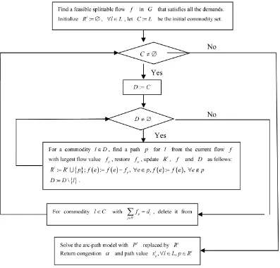
In this paper, we assume that there is a feasible splittable flow f that satisfies all the demands of the commod-ities. We know that f may not meet all the path number restrictions of the commodities. In [1], we find at most kl paths for commodity l from f , and then reallocate flow to the unsatisfied commodities by solving a series of linear programming. In this paper, we also find paths for commodity l from f . On the one hand, we finds paths for each commodity until the total path value is equal to its demand, on the other hand, for sake of fairness of different commodities, we find at most one path for each commodity in a round. The steps of the algorithm are as follows and the flow chart of the algorithm is presented inFigure 1.
Step 1: Find a feasible splittable flow f in G that satisfies all the demands; Initialize Rl:= ∅ for all
l∈L, denoting the paths found from f for commodity l;
Step 2: For l=1,,L , if the total path value of the paths in Rl is less than dl, find a path from the cur-rent flowf for commodity l that carry the largest flow value. Add the new path with its flow value to Rl. Once a path is found, delete its flow from f , update the edge flow values in f ;
Figure 1. The flow chart of the heuristic algorithm. In the process of the algorithm, when the total path value already found for some commodity equals to its demand, we will not find paths for it in the next round.
with l
P replaced by l
R . Remarks:
● In step 1, we can add a super sink node t to G, each sink node tl, l∈L is connected to t with capac-ity dl, denote the new graph by *
G . Finding f that satisfies all the demands of the commodities is equivalent to find the maximum s−t flow in *
G , since we assume the existence of f , the maximum
s−t flow in *
G is with flow value l l L∈ d
∑
and we can use any maximum flow algorithm to obtain the maximum s−t flow.● For each commodity l, the number of paths found is at most m and so the size of l
R is largely smaller than l
P . Since the existence of a feasible splittable flow f satisfying all demands, at the end of step 2 we have that f =0 and the total path value of l
R is dl for each l∈L.
● The new algorithm applies the Round Robin strategy to find paths. In each round, each commodity finds at most one path in the current flow f , this strategy guarantees some fairness in certain degree. To show the effectiveness of the Round Robin strategy, we compare our algorithm to the one that does not use the strate-gy in the next section. The computational results show that this stratestrate-gy does have some advantages for this problem.
4. Computational Results
those instances (seeTable 1) looks close to the transportation networks and may be well-suited for the MPLS networks. In this paper, we propose some results for the multi-commodity case. Tests were performed on an In-tel Core 2.4 GHz processor, 4 GB of RAM. We use CPLEX 12.5.1 to solve the arc-flow model. The running time of the CPLEX-solver is restricted to 50 seconds for each instance. The testing results are reported onTable 2 andTable 3.
In our testing, the total demands of the commodities in each instance are taken as the largest. While in prac-tice, the demand of each commodity may be much less than the amount we take, hence the congestions we ob-tained may be larger than 1. For simplicity, we denote the algorithm in [1] by H1. In this section, we also com-pare our algorithm to the one that not using the Round Robin strategy. That is the one which find paths from f
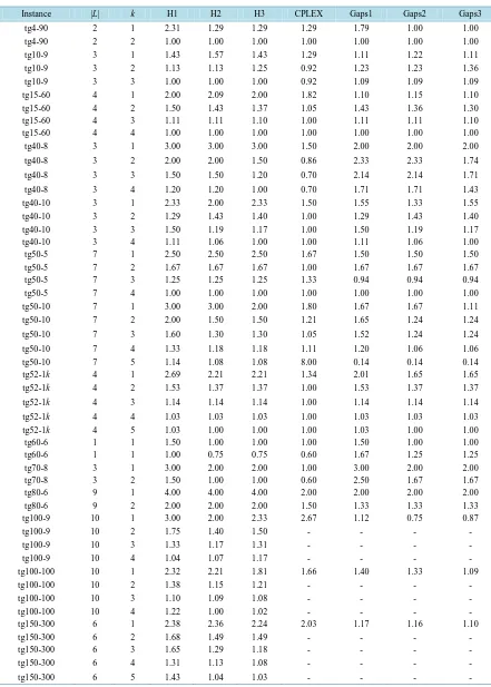
for each commodity until the total path values is its demand, and then go to the next commodity, denote the al-gorithm by H2. The new alal-gorithm proposed in this paper is denoted by H3. InTable 2, for each instance name, the first column followed is the number of commodities, and then followed the number of paths each commodity can use, and the next four columns are the congestions obtained by H1, H2, H3 and the CPLEX-solver in 50 seconds, and the last three columns followed are the ratios between the congestions of each of the three heuristic algorithms and the CPLEX-solver for each instance. The empty positions inTable 2 andTable 3 are because of the size of the instance runs out of memory, and hence no results are given. InTable 3, the last four columns are the corresponding running times for each instance.
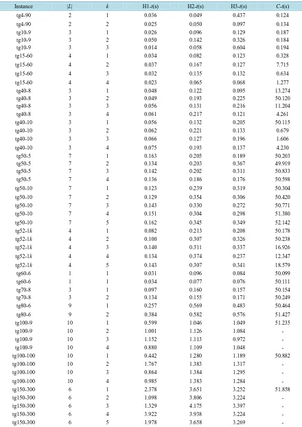
FromTable 3, we can note that the time spent for H1, H2 and H3 has little differences, all of the three heuris-tic algorithms run faster than the CPLEX-solver, and when the size of the instance or the number of paths that a commodity can use increases, the time spent for the CPLEX-solver has a big fluctuation, and most of the in-stances cannot obtain the exact solutions in the given time, we list the congestions obtained by the CPLEX- solver in 50 seconds. From column 4 and column 6 inTable 2, we can see that in the 50 test instances, 64% of the congestion values obtained by H3 is less than H1, and 30% have the same congestion values, and H1 has only 6% of the 50 congestion values that is less than H3. From column 5 and column 6 inTable 2, we note that 34% of the congestion values obtained by H3 are less than H2, and only 16% of the congestion values obtained by H2 are less than H3, this shows that the Round Robin strategy is useful in the heuristic algorithm. From the last three columns ofTable 2, we can note that for all the 40 sets of gaps, H1 has 24 instances that have gaps less than or equal to 1.5, while H3 has 31 instances with this property and H2 has 30. We can also note that H1 has 5 instances with gaps larger than 2 and H2 has 2 instances with this property, while H3 has no instance with gaps larger than 2. Hence we conclude that the performance of H3 outperforms H1 and H2. We know that in-creasing the size of path set for each commodity can minimize the congestion, but too large path set may also increasing the running time. So how to find paths for each commodity efficiently is a big challenge for this problem.
5. Conclusion
[image:6.595.88.540.584.720.2]In this paper, we consider the problem of minimizing congestion in the MPLS networks. We propose a new heuristic algorithm. This algorithm is based on the strategy that reduces the whole feasible path set for each commodity, and a Round Robin strategy is also used. The computational results show that the new algorithm is
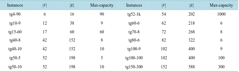
Table 1. Sizes of testing instances. For each instance name, the first column followed is the number of vertices, and then the number of edges and finally the maximum capacity of the edges in the instance.
Instances |V| |E| Max-capacity Instances |V| |E| Max-capacity
tg4-90 6 16 90 tg52-1k 54 202 1000
tg10-9 12 38 9 tg60-6 62 218 6
tg15-60 17 60 60 tg70-8 72 268 8
tg40-8 42 152 8 tg80-6 82 322 6
tg40-10 42 152 10 tg100-9 102 400 9
tg50-5 52 198 5 tg100-100 102 400 100
Table 2. The congestions obtained by the 3 testing heuristic algorithms and the CPLEX solver. The last three columns are the gaps between each of the 3 algorithms and the CPLEX-solver.
Instance |L| k H1 H2 H3 CPLEX Gaps1 Gaps2 Gaps3
tg4-90 2 1 2.31 1.29 1.29 1.29 1.79 1.00 1.00
tg4-90 2 2 1.00 1.00 1.00 1.00 1.00 1.00 1.00
tg10-9 3 1 1.43 1.57 1.43 1.29 1.11 1.22 1.11
tg10-9 3 2 1.13 1.13 1.25 0.92 1.23 1.23 1.36
tg10-9 3 3 1.00 1.00 1.00 0.92 1.09 1.09 1.09
tg15-60 4 1 2.00 2.09 2.00 1.82 1.10 1.15 1.10
tg15-60 4 2 1.50 1.43 1.37 1.05 1.43 1.36 1.30
tg15-60 4 3 1.11 1.11 1.10 1.00 1.11 1.11 1.10
tg15-60 4 4 1.00 1.00 1.00 1.00 1.00 1.00 1.00
tg40-8 3 1 3.00 3.00 3.00 1.50 2.00 2.00 2.00
tg40-8 3 2 2.00 2.00 1.50 0.86 2.33 2.33 1.74
tg40-8 3 3 1.50 1.50 1.20 0.70 2.14 2.14 1.71
tg40-8 3 4 1.20 1.20 1.00 0.70 1.71 1.71 1.43
tg40-10 3 1 2.33 2.00 2.33 1.50 1.55 1.33 1.55
tg40-10 3 2 1.29 1.43 1.40 1.00 1.29 1.43 1.40
tg40-10 3 3 1.50 1.19 1.17 1.00 1.50 1.19 1.17
tg40-10 3 4 1.11 1.06 1.00 1.00 1.11 1.06 1.00
tg50-5 7 1 2.50 2.50 2.50 1.67 1.50 1.50 1.50
tg50-5 7 2 1.67 1.67 1.67 1.00 1.67 1.67 1.67
tg50-5 7 3 1.25 1.25 1.25 1.33 0.94 0.94 0.94
tg50-5 7 4 1.00 1.00 1.00 1.00 1.00 1.00 1.00
tg50-10 7 1 3.00 3.00 2.00 1.80 1.67 1.67 1.11
tg50-10 7 2 2.00 1.50 1.50 1.21 1.65 1.24 1.24
tg50-10 7 3 1.60 1.30 1.30 1.05 1.52 1.24 1.24
tg50-10 7 4 1.33 1.18 1.18 1.11 1.20 1.06 1.06
tg50-10 7 5 1.14 1.08 1.08 8.00 0.14 0.14 0.14
tg52-1k 4 1 2.69 2.21 2.21 1.34 2.01 1.65 1.65
tg52-1k 4 2 1.53 1.37 1.37 1.00 1.53 1.37 1.37
tg52-1k 4 3 1.14 1.14 1.14 1.00 1.14 1.14 1.14
tg52-1k 4 4 1.03 1.03 1.03 1.00 1.03 1.03 1.03
tg52-1k 4 5 1.03 1.00 1.00 1.00 1.03 1.00 1.00
tg60-6 1 1 1.50 1.00 1.00 1.00 1.50 1.00 1.00
tg60-6 1 1 1.00 0.75 0.75 0.60 1.67 1.25 1.25
tg70-8 3 1 3.00 2.00 2.00 1.00 3.00 2.00 2.00
tg70-8 3 2 1.50 1.00 1.00 0.60 2.50 1.67 1.67
tg80-6 9 1 4.00 4.00 4.00 2.00 2.00 2.00 2.00
tg80-6 9 2 2.00 2.00 2.00 1.50 1.33 1.33 1.33
tg100-9 10 1 3.00 2.00 2.33 2.67 1.12 0.75 0.87
tg100-9 10 2 1.75 1.40 1.50 - - - -
tg100-9 10 3 1.33 1.17 1.31 - - - -
tg100-9 10 4 1.04 1.07 1.17 - - - -
tg100-100 10 1 2.32 2.21 1.81 1.66 1.40 1.33 1.09
tg100-100 10 2 1.38 1.15 1.21 - - - -
tg100-100 10 3 1.10 1.09 1.08 - - - -
tg100-100 10 4 1.22 1.00 1.02 - - - -
tg150-300 6 1 2.38 2.36 2.24 2.03 1.17 1.16 1.10
tg150-300 6 2 1.68 1.49 1.49 - - - -
tg150-300 6 3 1.65 1.29 1.18 - - - -
tg150-300 6 4 1.31 1.13 1.08 - - - -
Table 3. Running times of the 3 test algorithms and the CPLEX solver.
Instance |L| k H1-t(s) H2-t(s) H3-t(s) C-t(s)
tg4-90 2 1 0.036 0.049 0.437 0.124
tg4-90 2 2 0.025 0.050 0.097 0.134
tg10-9 3 1 0.026 0.096 0.129 0.187
tg10-9 3 2 0.050 0.142 0.326 0.184
tg10-9 3 3 0.014 0.058 0.604 0.194
tg15-60 4 1 0.034 0.082 0.123 0.328
tg15-60 4 2 0.037 0.167 0.127 7.715
tg15-60 4 3 0.032 0.135 0.132 0.634
tg15-60 4 4 0.023 0.065 0.068 1.277
tg40-8 3 1 0.048 0.122 0.095 13.274
tg40-8 3 2 0.049 0.193 0.225 50.120
tg40-8 3 3 0.056 0.131 0.216 11.204
tg40-8 3 4 0.061 0.217 0.121 4.261
tg40-10 3 1 0.056 0.132 0.205 50.115
tg40-10 3 2 0.062 0.221 0.133 0.679
tg40-10 3 3 0.066 0.127 0.196 1.606
tg40-10 3 4 0.075 0.193 0.137 4.230
tg50-5 7 1 0.163 0.205 0.189 50.203
tg50-5 7 2 0.134 0.203 0.367 49.919
tg50-5 7 3 0.142 0.202 0.311 50.833
tg50-5 7 4 0.136 0.186 0.176 50.598
tg50-10 7 1 0.123 0.239 0.319 50.304
tg50-10 7 2 0.129 0.354 0.306 50.420
tg50-10 7 3 0.143 0.330 0.272 50.771
tg50-10 7 4 0.151 0.304 0.298 51.380
tg50-10 7 5 0.162 0.345 0.349 52.142
tg52-1k 4 1 0.082 0.213 0.208 50.178
tg52-1k 4 2 0.100 0.307 0.326 50.238
tg52-1k 4 3 0.140 0.311 0.337 16.926
tg52-1k 4 4 0.134 0.374 0.237 12.347
tg52-1k 4 5 0.143 0.307 0.341 18.579
tg60-6 1 1 0.031 0.096 0.084 50.099
tg60-6 1 1 0.034 0.077 0.076 50.111
tg70-8 3 1 0.097 0.160 0.157 50.154
tg70-8 3 2 0.134 0.155 0.171 50.249
tg80-6 9 1 0.257 0.569 0.483 50.464
tg80-6 9 2 0.384 0.582 0.576 51.427
tg100-9 10 1 0.599 1.046 1.049 51.235
tg100-9 10 2 1.001 1.126 1.084 -
tg100-9 10 3 1.152 1.113 0.972 -
tg100-9 10 4 0.880 1.109 1.048 -
tg100-100 10 1 0.442 1.280 1.189 50.882
tg100-100 10 2 1.767 1.383 1.317 -
tg100-100 10 3 0.864 1.384 1.295 -
tg100-100 10 4 0.985 1.383 1.284 -
tg150-300 6 1 2.378 3.651 3.252 51.858
tg150-300 6 2 1.098 3.806 3.224 -
tg150-300 6 3 1.329 4.175 3.397 -
tg150-300 6 4 3.922 3.938 3.224 -
much better than the algorithm that we proposed before. One main limitation of the new algorithm is that it needs to solve a mixed integer linear programming, when the number of commodities is sufficiently large, the running time of the algorithm may be large. However, the idea of the algorithm provides a good feasible direc-tion for solving this problem. In the future, we will continue to do research on how to find better feasible path set for each commodity, not only this, we will design effective strategies to solve the mixed integer linear pro-gramming more quickly.
Acknowledgements
The work is supported by the National Natural Science Foundation of China under Grant No. 71171189, the key project of the National Natural Science Foundation under Grant No. 11331012 and the national key basic re-search development plan (973 Plan) project under Grant No. 2011CB706901.
References
[1] Jiao, C.W., Yang, W.G. and Gao, S.X. (2014) The k-Splittable Flow Model and a Heuristic Algorithm for Minimizing Congestion in the MPLS Networks. International Conference on Natural Computation (ICNC2014), Xiamen Univer-sity, 19-21 August 2014.
[2] Baier, G., Köhler, E. and Skutella, M. (2005) The k-Splittable Flow Problem. Algorithmica, 42, 231-248.
http://dx.doi.org/10.1007/s00453-005-1167-9
[3] Kleinberg, J.M. (1996) Single-Source Unsplittable Flow. Proceedings of the 37th Annual Symposium on Foundations of Computer Science, 68-77.
[4] Koch, R., Skutella, M. and Spenke, I. (2008) Maximum k-Splittable s,t-Flows. Theory of Computing Systems, 43, 56- 66. http://dx.doi.org/10.1007/s00224-007-9068-8
[5] Kolliopoulos, S.G. (2005) Minimum-Cost Single-Source 2-Splittable Flow. Information Processing Letters, 94, 15-18.
http://dx.doi.org/10.1016/j.ipl.2004.12.009
[6] Salazar, F. and Skutella, M. (2009) Single-Source k-Splittable Min-Cost Flows. Operations Research Letters, 37, 71- 74. http://dx.doi.org/10.1016/j.orl.2008.12.004
[7] Truffot, J., Duhamel, C. and Mahey, P. (2005) Using Branch-and-Price to Solve Multicommodity k-Splittable Flow Problem. The Proceedings of International Network Optimisation Conference (INOC), Lisbonne, 20-23 March 2005.
[8] Truffot, J. and Duhamel, C. (2008) A Branch and Price Algorithm for the k-Splittable Maximum Flow Problem. Dis-crete Optimization, 5, 629-646. http://dx.doi.org/10.1016/j.disopt.2008.01.002
[9] Gamst, M., Jensen, P.N., Pisinger, D. and Plum, C. (2010) Two- and Three-Index Formulations of the Minimum Cost Multicommodity k-Splittable Flow Problem. European Journal of Operational Research, 202, 82-89.
http://dx.doi.org/10.1016/j.ejor.2009.05.014
[10] Gamst, M. and Petersen, B. (2012) Comparing Branch-and-Price Algorithms for the Multi-Commodity k-Splittable Maximum Flow Problem. European Journal of Operational Research, 217, 278-286.
http://dx.doi.org/10.1016/j.ejor.2011.10.001
[11] Gamst, M. (2013) A Decomposition Based on Path Sets for the Multi-Commodity k-Splittable Maximum Flow Prob- lem. Department of Management Engineering, Technical University of Denmark, DTU Management Engineering Re-port No. 6.
[12] Edmonds, J. and Karp, R.M. (1972) Theoretical Improvements in Algorithmic Efficiency for Network Flow Problems.
Journal of the ACM, 19, 248-264. http://dl.acm.org/citation.cfm?id=321699
http://dx.doi.org/10.1145/321694.321699
currently publishing more than 200 open access, online, peer-reviewed journals covering a wide range of academic disciplines. SCIRP serves the worldwide academic communities and contributes to the progress and application of science with its publication.
Other selected journals from SCIRP are listed as below. Submit your manuscript to us via either