Optimizing Outdoor Propagation Model based on
Measurements for Multiple RF Cell
Allam Mousa
Department of Electrical Engineering An-Najah National University, Nablus,
Palestine.
Yousef Dama
Department of Electrical Engineering An-Najah National University, Nablus,
Palestine.
Mahmoud Najjar
Department of ElectricalEngineering
An-Najah National University, Nablus,
Palestine.
Bashar Alsayeh
Department of ElectricalEngineering An-Najah National University, Nablus,
Palestine.
ABSTRACT
This paper intends to study outdoor RF attenuation path loss behavior under certain restrictions. The study has been conducted in Nablus city to develop and optimize a suitable propagation model based on one of the existing propagation models based on outdoor measurements for 900 MHz, where a local GSM system is operating under sever geographical terrains and frequency limitations. The optimized model has been chosen such that certain error parameters are minimized. Some of the proposed models are; Bertoni-Walfish, Hat, Walfisch-Ikegami and the standard macrocell. In this paper a Tuned Bertoni-Walfisch model has outperformed the other models and has proven, tobe the best suited for propagation analysis involving such terrain. This is achieved by varying the range dependence using Least Mean Square Error (LMSE) method
Keywords
Multipath channel, radio channel modeling, Path loss model, Propagation measurements, Bertoni-Walfisch model, GSM 900.
1.
INTRODUCTION
Propagation, or path loss, models are basically used to predict coverage area, frequency assignment and interference, which are the main concerns in cellular network planning. The generalization of these models, to any environment, is suitable for either particular areas (urban, suburbs and rural), or specific cell radius (macrocell, microcell, picocell) depending on the diversity of environment where mobile communications occur. In general, there is a relationship between these models and types of environments for which they are suitable. The models can be any of the three types, namely the empirical modes (like Okumora and Hata models), semi-empirical models (like Cost-231 and Walfish-Ikegami models) and deterministic models (Maxwell’s Eq.) which are site specific and require enormous number of geometry information about the location. The empirical models’ parameters can be adjusted or tuned according to a targeted environment. The propagation model tuning must optimize the model parameters in order to achieve minimal error between predicted and measured signal strength. This will make the model more accurate for received signal predictions [1].
Usually, operators use special planning software like ASSET and ATOLL, to accomplish propagation model tuning [1], [2]. A Palestinian mobile communication operator, which operates
at GSM900, uses ASSET software which uses Standard Macrocell model, based on modified Hata model.
2.
Terrestrial description of Nablus city
and Survey Analyses
The city of Nablus cast narrow streets and moderately high buildings, the buildings heights vary between 9 and 12 m within the old city and city center Most of the buildings are mass of concrete, rock-like blocks, and bricks
The city is surrounded by two mountains from north with approximate height of 950 m and from the south with approximate height of 881 m and they are separated by around 2 km.
Extensive experimental tests were performed in the geographic area of Nablus and especially in the city center. The aim of these tests was to investigate the RF propagation in different directions relative to the streets. The results of those measurements were used to define the standard deviation, mean and RMSE, such that these values will be used to obtain a better understanding of wave propagation in the city.
In this section, the steps of collecting measurements, the equipment used and the statistical analyses of the measurements are presented. The main idea of the statistical analyses is to understand the radio wave propagation behavior for Nablus city at 900 MHz and finally to compare them with the applicable propagation models.
The data measurement equipments consist of a laptop equipped with TEMS software, a test mobile phone and a Global Positioning system (GPS). This tool can measure data in real time which can provide information about the network performance.
Due to a last fail test, we need to repeat this test with the same cell. But at this time, we turned off the neighboring 6 cells which have the same frequency at midnight. Where we cannot turning off the cells during day, because cells are busy so the most of capacity of cells are full enough. So, the number of samples became larger and the range of distance is wider. The received power ranges from -35 dBm to -120 dBm with distance ranges between 4 m and 521 m with 50748 samples. The specifications of the tested base station are illustrated in Table 1.
Table 1: Macrocell information.
Antenna Name XPol A-Panel 806–960 12.5dBi
Type No. 739 620
Channel No. (BCCH) 111 Frequency (BCCH) 957.2 MHz
PTX 45 dBm
GTX 2 x 12.5 dBi
EIRP 48.9 dBm
Azimuth 120o
Height 12 m
Down tilt (total) 10o
Feeder length 15 m
The measured values of the received signal strength are illustrated in Fig. 1.
Fig.1: Received power distribution for BS1.
The coverage prediction map of Standard macrocell model based in Hata model using ASSET software with received power (dBm) sampling is shown in Fig.2
Fig.2: Prediction map of BS1 for ASSET software and drive test samples.
3.
PROPAGATION MODELS
3.1
Standard Macrocell model
The Standard Macrocell model incorporates an optimal dual slope loss model with respect to distance from the base station. It also incorporates algorithms for effective base station heights, diffraction loss, and the effects of clutter. The general path loss (PL) formula for the Macrocell models is as follows [7];
1 2 3 4
5 6 7
( ) log( ) ( ) log( )
log( ) log( ) log( ) ( )
ms ms
eff eff loss
Path Loss dB k k d k H k H
k H k H d k diffin C
(1)
Where: d is the distance from the base station to the mobile station (km); Hms is the height of the mobile station above ground (m); Heff is the effective base station antenna height (m); diffn is the diffraction loss calculated using either the Epstein-Peterson, Bullington, Deygout or Japanese Atlas knife edge techniques; k1 and k2 are intercept and slope. These factors correspond to a constant offset (in dB) and a multiplying factor for the log of the distance between the base station and mobile; k3 is mobile Antenna Height Factor. Correction factor used to take into account the effective mobile antenna height; k4 is multiplying factor for Hms; k5 is
Effective Antenna Height Gain. This is the multiplying factor for the log of the effective antenna height; k6 is the multiplying factor for log (Heff)log (d); k7 is the multiplying factor for diffraction loss calculation; C_loss is the clutter specifications taken into account in the calculation process. The propagation model can be tuned by modifying the k-factors. For improved near and far performance, dual slope attenuation can be introduced by specifying both near and far values for k1 and k2, and the crossover point.
3.2
Log-distance propagation model
The Log – distance propagation model is based on the theory that; the average received signal power decreases logarithmically with distance (d) between the transmitter and the receiver [8-9]. This can be expressed as;
( ) o 10 log( / o)
PL dB L n d d (2)
Where, L =32.4+20log (f)+20log (d ) is the reference 0 10 10 o path loss, n is the path loss exponent (usually empirically determined by filed measurement), d0 is the reference distance in (km), d is the distance between transmitter and receiver in (km). Table 2 gives some typical values of n, larger values of n correspond to more obstructions and hence faster decreases in average received power as distance becomes larger [8].
[image:2.595.56.290.589.723.2]Table 2: Path Loss Exponents for Different Environments
Environment Path Loss Exponent , n In building line-of-sight 1.6 to 1.8
Free Space 2
Obstructed in factories 2 to 3 Urban area cellular radio 2.7 to 3.5 Shadowed urban cellular radio 3 to 5
Obstructed in building 4 to 6
This model implementation may be achieved by Choosing d0 = 1 (m) as a reference, one may apply this model to measure and calculate the path loss exponent n (Eq.2). This value is found to be 3.86 which mean that BS1 is located in shadowed urban area as discussed in Table 2. Hence, the Log-distance propagation model may be re-written as;
( ) o 38.6log o d
PL dB L
d
(3)
[image:3.595.320.535.233.315.2]The Simulation results for this propagation model and the measured values are illustrated in Fig. 3. Moreover, applying this model for other cells to find path loss exponent n is illustrated in Table 3, where the main statistical indications (Mean Error µ, Standard Deviation σ, Root Mean Square Error (RMSE)) for Log-distance propagation model values compared to the measured ones are illustrated in Table 4.
Fig.3: Log-distance model at n=3.86 and measured data.
Table 3: Path loss exponent for different base stations.
Cell No. 1 2 3 4 5 6 7 8
Path Loss exponent
(n)
3.86 3.9 3.6 3.82 4.16 3.64 3.91 4.41
Table 4: Statistical values for Log-distance propagation model applied for certain base stations.
Base station
No.
# of samples
Mean error
Standard
deviation RMSE
BS1 50748 2.11 13.14 13.31 BS2 4163 2.22 13.864 14.04
BS3 9627 0.22 8.8 8.8116
BS4 8336 0.72 11.396 11.4186 BS5 21390 1.473 11.628 11.721
BS6 3968 0.1547 5.9 5.92
BS7 3937 0.444 9.414 9.423
BS8 2652 0.335 9.06 9.065
Table 3 indicates typical n values referring to all base stations located in shadowed urban area which is true as discussed in Table 2.
3.3
Bertoni-Walfisch propagation model
Bertoni-Walfisch proposed a semi empirical model that is applicable to propagation though buildings in urban environments. Which, it has been adopted here due to its simplicity and validity which has been verified with measurements [10]. The model assumes building heights to be uniformly distributed and the separation between buildings are equal. Propagation is then equated to the process of multiple-diffraction past these rows of buildings. The building geometry and parameters in Bertoni-Walfisch model are illustrated in Fig. 4.
Fig.4: The building geometry and parameters in Bertoni-Walfisch Model.
The path loss formula for Bertoni-Walfisch propagation Model is given as [3], [4];
( ) 89.5 38log( ) 18log( t b) 2log( ) PL dB A d h h f (4) Where,
2 2
1
5log ( ) 9log( ) 20log tan
2
h h
b b m
A hb hm b
b
d :Distance between base station and the mobile in km. f :Frequency in MHz
ht :Antenna Height in meters. hb :Building height in meters. hm :Mobile height in meters.
b :center-to-center spacing of the rows of the buildings in meters
In propagation studies, there are many propagation models especially in urban areas like (Hata, Haret, COST231 Walfisch-Ikegami, and Bertoni-Walfisch) [8], to choose the most accurate one, we applied many of them to compar the performance with the measured data (BS1) then we made a comparison between them to check which one has a minimum error. Some of the statistical indicators are illustrated in Table 5 for the widely used propagation models.
Table 5: Mean error, standard deviation and RMSE for various models for BS1.
Empirical Propagation
model
Mean error (dB)
Stand ard devia tion
RMS E
Hata 12.598 12.96 18.07 5 Haret 10.348 12.98 16.6 COST231
Walfisch- Ikegami
10.58 12.99 16.76
[image:3.595.71.266.368.498.2]From Table 5, one can notice that Bertoni-Walfisch is the best model, under our circumstances, since it has the minimum mean error and minimum RMSE. Hence, in order to improve the performance of this model (increase its accuracy), it is aimed to tune it using certain techniques like Least Mean Square Error (LMSE).
4.
OPTIMIZATION PROCESS
[image:4.595.321.540.69.247.2]The optimization, or tuning, process is based on the measured data using least square method. Statistical analysis such as mean error, standard deviation and root mean error were used. Comparison between optimized model and other models were compared according to these statistical values. An illustrative block diagram is shown in Fig.5 [11].
Fig.5: Block diagram of optimization process.
4.1
STANDARD MACROCELL MODEL
TUNING
The Standard Macrocell model has been tuned by applying LMSE on the path loss equation given in Eq.1, the tuned model can be written as;
( ) 139.41 30log( ) 2.55( ) 0log( ) 13.82log( ) 6.55log( )log( ) 0.7( )
PL dB d Hms Hms
Heff Heff d diffn CLoss
(5)
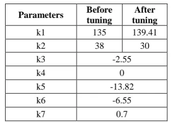
The k factors of the model were tuned such that the obtained values for k1 and k2 are 139.41 and 30 respectively to replace the unturned values of 135 and 38, the values of k3 – k7 remains unchanged as shown in Table 6.
Table 6: Model parameters before and after tuning
Parameters Before tuning
After tuning
k1 135 139.41
k2 38 30
k3 -2.55
k4 0
k5 -13.82
k6 -6.55
k7 0.7
[image:4.595.57.281.222.296.2]The path loss of measured data and Macrocell model before tuning versus tuned model is shown in Fig.6. The tuned model represents the measured data with less mean error.
Fig.5: Path loss comparison of Standard macrocell model before and after tuning for BS1.
4.2
BERTONI-WALFISCH MODEL
TUNING
Optimization of the Bertoni-walfisch Model is based on minimizing the LMSE between the best fit of the model and the practically measured data as given in Eq. 6 [11].
1
[ ( , , , ,...)] min N
i R i i
y E x a b c
(6)yi = measurement result at the distance xi.
ER (xi; a; b; c;) = modeling result at the xi based on optimization.
a; b; c = parameter of the model based on optimization; n = Number of the experiment data set.
Accordingly, the tuned Bertoni-Walfisch model is tuned to; ( ) 78.5 23log( ) 18log(t b) 21log( ) PL dB A d h h f (7) Based on the Bertoni-Walfisch model, the Simulation results are illustrated for the original and tuned model in terms of path loss as shown in Fig. 7. From Eq. (7), one can see that, the path loss increases with distance at a rate of 23 dB per decade in Bertoni-Walfisch model after tuning.
[image:4.595.82.256.471.591.2] [image:4.595.330.524.533.695.2]The statistical analysis calculated were for the merits of Mean error µ, Standard deviation σ and Root Mean Square Error (RMSE) [12], [13], [14]. Where, error is the difference between measured and predicted values of tuned Bertoni-Walfisch model. The results of the statistical analysis for Bertoni-Walfisch model and Standard Macrocell model are given in the Table 7.
Table 7 Mean error, standard deviation and RMSE comparison for Bertoni-Walfisch and Standard Macrocell
models
µ (dB) Σ RMSE
Before tuning After tuning Before tuning After tuning Before tuning After tuning Bertoni-Walfisch
1.426 0 13 11.294 13.07 11.294
Standard Macrocell model
10.91 0 11.792 11.294 16.06 11.294
5.
Simulation and Results
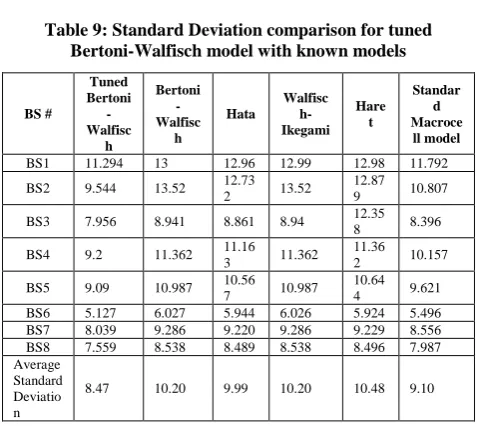
[image:5.595.309.548.179.392.2]The tuned Bertoni-walfisch model has been applied for 8 base stations in Nablus. Where, multiple cell implementations have been conducted. The performance has been compared to several other models like Hata, Walfish-Ikegami, Hata and standard Macrocell. Comparison has been performed in terms of error and standard deviation as shown in Table 8 and Table 9 respectively. The comparison shows that the proposed tuned Bertoni-Walfisch tuned model is suitable for almost all the base stations since the error was reduced significantly. The proposed tuned model has been compared to other models as shown in Fig.8. The mean error of BS1 has been reduced to zero and the standard deviation was decreased by 13.12% and the average standard deviation is 8.47.
Fig.8: Path loss comparison between measured data for BS 1 and propagation models.
Table 8: Mean Error comparison between tuned Bertoni-Walfisch models with known models
BS # Tuned Bertoni -Walfisc h Bertoni -Walfisc h Hata Walfisch -Ikegami Haret Standar d Macroce ll model
BS1 0 1.426 12.59
8 10.58
10.34
8 10.91
BS2 6.978 10.728 17.82 16.5 10.32
9 18.536
BS3 2.367 9.633 9.737 10.106 8.636 12.067
BS4 3.254 6.941 14.72 11.697 10.96 14.510
6 6
BS5 13.041 12.32 23.11
7 18.936
15.76
9 21.774
BS6 3.342 11.576 10.78
9 11.083 9.707 13.565
BS7 5.88 8.891 16.42
4 14.322
13.56
7 16.797
BS8 16.813 16.311 27.21
4 25.255
24.37
7 25.971
Averag e Mean Error
[image:5.595.47.288.185.276.2]6.64 9.55 16.55 14.80 12.96 16.76
Table 9: Standard Deviation comparison for tuned Bertoni-Walfisch model with known models
BS # Tuned Bertoni -Walfisc h Bertoni -Walfisc h Hata Walfisc h-Ikegami Hare t Standar d Macroce ll model
BS1 11.294 13 12.96 12.99 12.98 11.792
BS2 9.544 13.52 12.73
2 13.52
12.87
9 10.807
BS3 7.956 8.941 8.861 8.94 12.35
8 8.396
BS4 9.2 11.362 11.16
3 11.362
11.36
2 10.157
BS5 9.09 10.987 10.56
7 10.987
10.64
4 9.621
BS6 5.127 6.027 5.944 6.026 5.924 5.496
BS7 8.039 9.286 9.220 9.286 9.229 8.556
BS8 7.559 8.538 8.489 8.538 8.496 7.987
Average Standard Deviatio n
8.47 10.20 9.99 10.20 10.48 9.10
6.
CONCLUSION
This paper investigates the optimization of path loss model using least square method. The outdoor measurements was taken in Nablus city, which is an urban area with geographical and frequency shortage limitations. The tuning has been conducted to make a path loss comparison with the existing models. Results from the analysis and measurements reported her lead to the conclusion that the performance of the tuned Bertoni-Walfisch model is the best among the tested ones. Fine tuning of the Bertoni-Walfisch model and Standard Macrocell model are carried out using Linear Least Square method on large number of measurement records. The mean Error value for BS 1 has been reduced to zero and the standard deviation values were reduced by 13.15% and 4.2% for Bertoni-Walfisch model and Standard Macrocell model respectively. Hence, this tuned Bertoni-Walfisch propagation model is proposed to improve the performance and so it may be used for propagation prediction in the city.
7.
REFERENCES
[1] Mingjing Yang, Wenxiao Shi. “A Linear Least Square Method of Propagation Model Tuning for 3G Radio Network Planning”, Vehicular Technology Conference, 2008. VTC 2008-Fall, IEEE 68th, Calgary, pp.150-154 [2] Liu Yang, Wand Fang, Chang Yongyu; YANG
Da-cheng. “Theoretical and Simulation Investigation on Coexistence between TD-SCDMA and WCDMA system”, Vehicular Technology Conference, IEEE, Dublin, 2007, pp.1198-1203.
[image:5.595.56.277.424.596.2][4] Alvaro Valcarce, Jie Zhang, “Empirical Indoor-to-Outdoor Propagation Model for Residential Areas at 0.9– 3.5 GHz”, IEEE ANTENNAS AND WIRELESS PROPAGATION LETTERS, VOL. 9, 2010
[5] Leandro Fernandes, Antonio Soares, “Simplified Characterization of the Urban Propagation Environment for Path Loss Calculation”, IEEE ANTENNAS AND WIRELESS PROPAGATION LETTERS, VOL. 9, 2010 [6] R. Mardeni, K. F. Kwan, “Optimization of Hata
Propagation Prediction Model in Suburban Area in Malaysia”, Progress In Electromagnetics Research C, Vol. 13,pp. 91-106, 2010
[7] ASSET, User Reference Guide, Software Version 6.1, Reference Guide Edition 1. V 6.0 is available online on http://www.scribd.com/doc/19033329/ASSET-User-Reference-Guide [Accessed in April 2010].
[8] James Demetriou, Rebecca MacKenzie. “Propagation Basics”, September 30, 1998, pp.39-42. Available online on http://www.scribd.com/doc/7218261/Propagation-Basics [Accessed in April 2010].
[9] B.Yesim HANCI, I.Hakki CAVDAR. “Mobile Radio Propagation Measurements and Tuning the Path Loss Model in Urban Areas at GSM-900 Band in Istanbul – Turkey”, Fall 60th Vehicular Technology Conference IEEE Vehicular Technology Conference No60, Los Angeles CA , ETATS-UNIS, pp. 139-143, 2004.
[10]M. A. Alim, M. M. Rahman, M. M. Hossain, A. Al-Nahid. “Analysis of Large-Scale Propagation Models for Mobile Communications in Urban Area”, International Journal of Computer Science and Information Security, Vol. 7, No. 1, pp.135-139, 2010.
[11]R. Mardeni, K. F. Kwan, “Optimization of Hata Propagation Prediction Model in Suburban Area in Malaysia”, Progress In Electromagnetics Research C, Vol. 13, pp. 91-106, 2010
[12]Jianhui Wu, Dongfeng Yuan. “Propagation Measurements and Modeling in Jinan City”. Personal, Indoor and Mobile Radio Communications, The Ninth IEEE International Symposium, Sendai, Japan. pp. 1157 - 1160 vol.3, 1998.
[13]Faihan D. Alotaibi, Adel A. Ali. “Tuning of Lee path loss model based on recent RF measurements in 400 MHz conducted in Riyadh city, Saudi Arabia”. The Arabian Journal for Science and Engineering, Vol. 33 Number 1B, pp.145-152, April 2008.