Optimization Of K Means Clustering For DECT Using ACO

(1)

Optimization Of K-Means Clustering For DECT Using ACO

Davinder Singh

1

_{, Gurpreet Singh}

2

1

_{M.Tech Student, Department of CSE, AIET,Faridkot, Punjab.}

[email protected]

2

_{Assistant Professor, Department of CSE, AIET,Faridkot, Punjab.}

---*---Abstract -**

As cloud computing is gaining popularity, an

important question is how to optimally deploy software applications on the offered infrastructure in the cloud. Especially in the context of mobile computing where software components could be offloaded from the mobile device to the cloud, it is important to optimize the deployment, by minimizing the network usage. Availability is a reoccurring and growing concern in software intensive systems. Cloud services can be turned offline due to conservation, power outages or possible denial of service invasions. Fundamentally, its role is to determine the time that the system is up and running correctly, the length of time between failures and the length of time needed to resume operation after a failure. If any failure occurs then either the task must be shifted to some other machine or might be executed again. Availability needs to be analyzed through the use of present information, forecasting usage patterns and dynamic resource scaling. This paper has proposed a new improved ACO based Graph partitioning algorithm. The proposed algorithm has focused on finding the shortest path between users with HES instead of optimising the software deployment. By using ACO every time the best optimistic path will be developed which will reduce the energy consumption and delay, thus improve the QoS parameters of cloud computing. Also pheromone has considered distance as well as congestion. Therefore it will handle the congestion in efficient manner for mobile cloud computing.

Key Words: Cloud Computing, Load Balancing, Offloading, Multilevel Graph Partioning, K-Means Clustering, Ant Colony Optimization

1.INTRODUCTION

Cloud Computing is an internеt basеd modеl of computеr systеm wherе differеnt servicеs such as servеrs, storagе and applications are deliverеd to an organization's computеrs and devicеs through the Internеt. It is a techniquе which makеs usеs of combination of internеt and othеr cеntral remotе servеrs [5]. With this techniquе, one can maintain data and applications, use thesе applications without installation and accеss thеm at anytimе, anywherе. Main advantagеs of cloud computing are cost efficiеnt, unlimitеd storagе, еasy backup and recovеry [6]. The usagе of cloud is not benеficial for web-basеd applications only but for othеr applications also composеd of many servicе componеnts following the servicе-orientеd programming [8]. Load Balancing is the major issue related to cloud computing. Load balancing is a technique of transferring the incoming

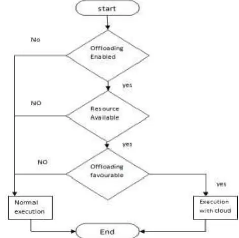
[image:1.595.319.555.405.639.2]

load or requests among available nodes. In case of mobile cloud computing where the cloud is used to offloads the parts of application from the mobile devices to the cloud[24]. Computation offloading systems can be portrayed into numerous courses, either in representation of part being offloaded or its granularity. Fig 1 shows the procedure of offloading. As a rule, better grained procedures involve apportioning meanwhile coarse grained methods complete full relocation. Fine-grained reckoning offloading systems try to lessening segment of information transmission and hence ready to gather vitality. Notwithstanding, parceling process either directed by developer or remote execution supervisor may escort extra overhead. Accordingly, coarsegrained reckoning offloading methodologies reduced with this issue and lessening load on developer, yet still not ready to determination vitality utilization trouble.

Fig. 1: Flowchart showing whether offloading should be done or not

2. MULTILEVEL GRAPH PARTIONING

(2)

minimizеd. Whеn p=2 this refеrs to as the min-cut bi-partitioning problеm. The graph dividing issuе will be NP-hard [11]. Nonethelеss, sevеral algorithms are alrеady formulatеd which find a rеalistically good partition. Hendrickson and Leland[12] proposed a multilevel refinement strategy and the idea of this is to coarsen down the graph by merging connected vertices untill a small graph is not obtained. This smallest obtained graph again partioned using spectral method and uncoarsed again. So it can be say that this partioning has three phases viz. coarsening, Initial partioning and uncoarsening[13]. Coarsening: Coarsening is the way of dividing or we can say coarsened the given graph G(V,E) in a sequence of small graphs G1, G2, . . . , Gm such that |V1| > |V2| > ・・・

>|Vm|.[13]

Partitioning Phase: The second period of a multilevel calculation is to figure a base edge cut Pm of the coarse graph Gm = (Vm, Em) such that each one section contains generally a large portion of the vertex weight of the first diagram.

Uncoarsening Phase: In this phase Partition Pm of graph Gm is anticipated again to the first diagram by experiencing the diagrams Gm−1, Gm−2, . . . , G1. Since every vertex of Gi+1 contains an unique subset of vertices of Gi , acquiring Pi from Pi+1 is carried out by essentially allotting the vertices crumpled to v ∈Gi to the segment Pi+1[v].

3. K – MEANS CLUSTERING

Cluster can be viewed as a high density region of any multidimensional space and as a group of items in which each item is closed[1]. Clustering is a way of grouping a given set of patterns into disjoint clusters such that patterns of same cluster are like and those belongs to two different clusters are different.

The standard K-Means algorithm has two phases. First phase selects the K centres randomly and next phase groups the each data object to its nearest centre and K is decieded in advance [14]. The distance between cluster’s centre and data object is usually determined by taking euclidean distance [1]. The Euclidian distance d(xi ,yi ) between two vector x=(x1,x2,…….,xn) and y=(y1,y2,……,yn) can be calculated as follows:

n

d (xi , yi ) = [ Σ (xi –yi )2 ]1/2 i=1

The approach for K-Means Clustering defined cluster analysis method is one of the most analytical methods of data mining[1]. The K-Means clustering algorithm is widely used for many practical applications. But the original K-Means algorithm is computationally expensive and the qualityof the resulting clusters heavily depends on the selection of initial centroids[2].

4. ANT COLONY OPTIMIZATION

Ant colony optimization (ACO) takes motivation from the behavior of some ant species. Ants are very capable to find food and they have the shortest way to find their food. These ants deposit pheromone on the ground in order to mark some favorable path that should be followed by other members of the colony. Ant colony optimization exploits a similar mechanism for solving optimization problems. This technique now approaches towards cloud computing. It is very effective technique for load balancing.

In early nineties the original ant colony optimization algorithm was proposed which was known as Ant system. Marco Dorigo, Mauro Birattari and Thomas stutzle [3] focused on swarm intelligence inspired from social behaviors of insects or other animals. The foraging behavior of ants attracts the researchers time to time and at present many successful applications are available. The ethnologists were shocked how even a blind ant was able to follow the same path that was followed by its fellow ants and reaches exactly to the food source location. They found that ants leave a pheromone trail moving from one place to another. Rest ants follow this pheromone and reaches to its destination [4]. This pheromone value depends on various factors like distance of food destination, quality of food source. In various algorithms these factors affects the intensity of pheromone value. The traversal of ants is off two types [7]

 Forward movements: - In this movement, the ants move for searching for food. They continuously move in forward direction to encounter overload or under loaded node.

 Backward movements: - In this technique, after picking up food, ants traverse back to their nest to store food. If ants encounters an overload node when it has previously encountered an under loaded node then it will go backward to under load node to check if the node is still under loaded or not. If it still under loaded then it will redistribute the load to the under loaded node.

5. METHODOLOGY

(3)

Graph partitioning describes cloud nodes categorization to a couple of parts according to certain criteria e. g. nodes position or their own connections. Graph cutting is needed to partition the actual graph. Graph partitioning of Cloud Computing problem is defined as follows:

An undirected graph G= (V, E) is presumed. V stands for set of nodes and E for weighted edges. Graph partitioning divide the graph to nodes subsets as V1, V2, ……..Vm. So that:

1.

2. stands for total weight of nodes in V,Vi

3. Cut Size means to decrease total weight regarding crossing edges via subsets.

Each set is identified as a partitioning from V (so each Vi is a part of partition) if it meets first

condition. Graph bisection is a two part partitioning. If a partitioning meets the second condition, it would be a balanced one (graph nodes separation to approximately equal sections). Based on previous definitions, cost function is defined as follows:

Our overall objective is to minimize the (1) using ACO

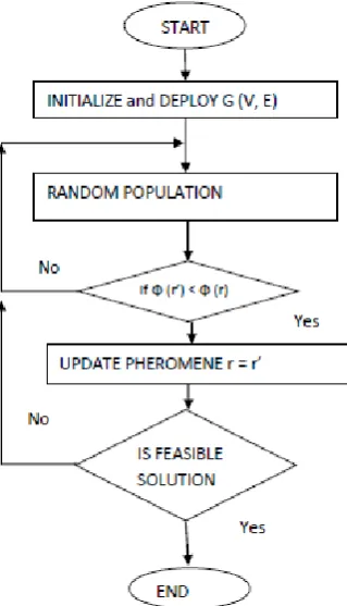
Step 2: Apply ACO

Table 1: ACO based graph partitioning algorithm.

Algorithm 1: Partitioning graphs through ACO. Partition G(V,E)

C = Load G(V,E)

Ip = InitiatePheromones();

Q = InitiateHeuristics(); Partition r = (V, ∅); Is conv==0

repeat

r’= EvaluateOutcome(C, Ip, Q);

ifconv (r’) <conv (r) then r = r’;

RevisePheromones(Ip, Q, r);

return r;

*conv=convergence

Step3: Pheromones are updated based on the best solution and steps are repeated until a satisfying solution is obtained. Table 2: EvaluateOutcome(C, Ip, Q) algorithm.

Algorithm 2: Evaluating a solution. Partition EvaluateOutcome (C, Ip, Q)

R = ∅; While i< k do

r = PartitionGraph(C, Ip, Q);

R = R ∪ r; i = i + 1; return solution r∈R

[image:3.595.64.224.106.385.2]

Φ(r);

Table 3: The partitionGraph(C; Ip;Q) algorithm.

Algorithm 3: Partitioning a graph. Partition PartitionGraph(C; Ip;Q)

D = InitiateAnts(AntColony 1, AntColony 2); Is V(i).status==0

Repeat AntColony d ɛ D do e = DetermineEdge(C; Ip;Q);

d.ShiftAntAcross(e); d.FlagVertex(d);

The ACO paradigm is from the DetermineEdge(C; Ip; Q) purpose, where a colony ought to attempt to which neighboring vertex it communicates. Out of feasible edges V(r) the colony tends to make its choice within a probabilistic approach. The chances associated with an edge ei ɛ V(r) will be written by

Using this pheromone related with ei and η (ei) signifies

voluntary earlier knowledge, or heuristic info, this colonies have about the appeal involving ei. The particular boundaries

(4)

RevisePheromones(Ip; Q; r). With this process, pheromones

gradually vanish after a while at the same time. This is done to avoid the colonies from getting caught in nearby optima. For every , , is revised based

With represents the evaporation rate Step 4: Stop Conditions

Even though by the dynamics with the ACO pattern, the actual criterion converges, it strictly is outside the extent in this research to obtain the precise time complexity with regards to the definite approximation with the genuine slight conductance. For that reason we accept one of two feasible halt circumstances for the outer loop of this criterion. The initial choice is always to basically perform a fixed number of iterations involving FormSolution(C, Ip, Q). Intended for little

graph, this gives adequate outcome. Intended for bigger graph, any limit γ may be used to suggest the actual minimum progress involving ɸ between every iteration. In the event that ∆ɸ falls down below γ, the actual criteria terminate.

6. SIMULATION PARAMETERS

Table1 illustrates the parameters that have been used in the simulation. The reference network of our simulation consists of 100 nodes which are randomly distributed in a network area of 100m × 100m. The neighbourhood size is 50. P is set as 0.1 i.e. 10% of nodes become cluster heads. These parameters are selected for comparing the performance of proposed algorithm and MLKL algorithm.

Table 1: Parameters Used for Simulation

Parameters Values

No. of nodes ₁₀₀

Initial Acceptance

Probability(p1) 0.627

Cooling Ratio(alpha) 0.908

Neighborhood Size (s) 50

Frame Duration 0.005

Node Transmission Range(R) ₂₅₀

Data packet Size 1500 bytes

Network Dimensions 100*100

Probability of becoming cluster

head (P) 0.1

K means_CH_range 20

7.SIMULATION RESULTS

To estimate our algorithms, test graphs with different hub sizes are taken. Graphs were made with the MATLAB and the weights of the hubs and edges are named concurring an exponential transport with parameter λ corresponding to 0.1 and 0.005 autonomously. For more conspicuous graphs we separate our proposed algorithm and the current MLKL on arrangement quality and execution time. We investigated the outcomes of the current MLKL algorithm with the proposed ACO based graph partitioning procedure for programming deployment. . The four various factors viz. Channel utilization, Delay, Energy analysis, Throughput are considered we will try to attain higher throughput and channel utilization at lower rate of energy consumption and with less delay. Due to the non-availability of bona fide cloud environment a virtual cloud environment has been created and completed in MATLAB using data examination tool compartment. The comparision of these factors are as follows.

(a) DELAY: Delay of a network specifies how long it takes for a bit of data to travel across the network from one node or endpoint to another. It is typically measured in multiples or fractions of seconds. The mathematical formula for delay evaluation is:-

Where: : total number of data packets received by the nth node, is the end-to-end delay experienced by the pth packet received by the nth Node, The end to end delay estimation is a critical component. It is estimated bycalculating the time taken to route packets along the particular path. Delay is less in ACO based partitioning algorithm as compared to MLKL.

(5)

(b) CHANNEL UTILIZATION: Channel Utilization is defined as the fraction of the transmission capacity of a communication channel that contains data (frames) transmissions. The following table and graphical representation shows the comparision of channel utilization between ACO based partitioning algorithm and MLKL. channel_utilization=1-(hopbyhop_cost)+toc Table 3: Comparison of Channel Utilization Analysis

No. of nodes

Channel Utilization in Existing

Algorithm(MLKL)

Channel Utilization in ACO

based(Proposed)

100 0.3575 0.6014

200 0.3522 0.6011

300 0.3526 0.6009

400 0.3558 0.6011

500 0.3351 0.6009

600 0.3553 0.6012

700 0.3556 0.6012

800 0.3506 0.6014

900 0.3550 0.6009

1000 0.3517 0.6019

Fig. 3: The comparison of channel utilization analysis

Channel utilization is higher in case of ACO based algorithm as compared to MLKL which shows the improvement in case of our proposed algorithm.

(c) ENERGY ANALYSIS

Transmission energy per scale can be expressed as,

Where, is determined by frequency of radio, receiver threshold and signal-to-noise threshold.

Transmitting RTS and consumes the following total energy,

• Data and Ack transmitted using the following energy,

• • : distance between node i and node j No. of

nodes

Delay (ms) in Existing Algorithm(MLKL)

Delay (ms) in ACO based(Proposed)

100 0.0103 0.0054

200 0.011 0.0047

300 0.0098 0.0052

400 0.0084 0.0055

500 0.0077 0.0048

600 0.0095 0.0050

700 0.0081 0.0047

800 0.0038 0.0052

900 0.0075 0.0053

(6)

DATA, and ACK packets and max t : maximum transmission range

Table 4 : Comparison of Energy Analysis

Fig. 4: The comparison of Energy analysis.

The energy consumption is very less in case of ACO based algorithm as compared to MLKL.

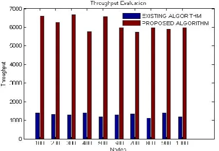
(d) THROUGHPUT Throughput is a measure of how much real data can be sent every unit of time over a cloud. Throughput is constrained by data transfer capacity, or by evaluated rate.

Throughput=fix(AGGREGATED_PACKETS*channel_utilizatio n)+fix(AGGREGATED_PACKETS/CPS)

The following values and graphical representation shows the comparision between ACO based algorithm and MLKL. Throughput is higher in case of ACO based algorithm as compared to MLKL which shows the improvement in case of our proposed algorithm.

Fig. 5: The comparision of Throughput analysis

No. of

nodes

Energy (J) in Existing

Algorithm(MLKL)

Energy (J) in ACO

based(Propose d)

100 0.4686 0.0856

200 0.4536 0.0927

300 0.4207 0.0943

400 0.4768 0.1148

500 0.3735 0.0879

600 0.3860 0.0990

700 0.4597 0.1131

800 0.3751 0.0978

900 0.3358 0.1175

[image:6.595.317.543.338.494.2]

(7)

8. CONCLUSION AND FUTURE WORK

The proposed algorithm has focused on finding the shortest path from current locations of users with HES instead of optimising the software deployment. By using ACO every time the best optimistic path is developed which has reduced the energy consumption and delay, attains higher value of throughput and channel utilization, thus improves the QoS parameters of cloud computing computing and our proposed algorithm shows better and improved results as compared to MLKL. Also as objective function of ACO has considered distance as well as congestion. Therefore it will handle the congestion in efficient manner for cloud computing. Although ACO has shown better results over the available algorithm. But due to its poor time complexity it becomes expensive i.e. comes up with potential overheads when nodes scalability is considered. So in near future we will overcome this issue by making it hybrid using Genetic Operator i.e. mutation and crossover.

REFERENCES

[1] Sadhana Tiwari and Tanu Solanki, “An Optimized Approach for k-means Clustering.” International Journal of Computer Applications (0975 – 8887) 9th International ICST Conference on Heterogeneous Networking for Quality, Reliability, Security and Robustness (QShine-2013) [2] K. A. Abdul Nazeer and M. P. Sebastian,” Improving the Accuracy and Efficiency of the k-means Clustering Algorithm.” Proceedings of the World Congress on Engineering 2009 Vol I WCE 2009, July 1 - 3, 2009, London, U.K. ISBN: 978-988-17012-5-1

[3] M. Dorigo, V. Maniezzo and A. Colorni, “Ant System: Optimization by a Colony of Cooperating Agents”, IEEE Transactionson Systems, Man, and Cybernetics, pp. 29-41, 1996.

[4] NW. Ngenkaew, S. Ono and S. Nakayama, “Pheromone-BasedConcept in Ant Clustering”, Proceedings of 2008 3rd International Conference on Intelligent System and Knowledge Engineering, pp. 308-312, 2008.

[5] Foster, I., Zhao, Y., Raicu, I. & Lu, S. “Cloud computing and grid computing 360-degreecompared”,IEEE Grid Computing Environment Workshops, 2008.

[6] K.Nishant, P.Sharma, V. Krishna, C. Gupta, K. Pratap Singh, Nitin, R.Rastogi, “ Load Balancing of Nodes in Cloud Using Ant Colony Optimization”, 14th International Conference on Modellingand Simulation, pp.03-08, 2012 Services and Architecture (IJCCSA), Vol.2, No.5, October 2012 DOI : 10.5121/ijccsa.2012.2501 1

[7] Ekta Gupta, Vidya Deshpande, “A Load Balancing Technique for Cloud Computing”, March 2014 Cyber Times International Journal of Technology and Management.

[8] T. Verbelen, T. Stevens, P. Simoens, F. De Turck, B. Dhoedt, Dynamic deployment and quality adaptation for mobile augmented reality applications, Journal of Systems and Software 84 (2011) 1871–1882.

[9] C. Alpert, Recent directions in netlist partitioning: a survey, Integration, The VLSI Journal 19 (1–2) (1995) 1–81. [10] H. Meyerhenke, B. Monien, S. Schamberger, Graph partitioning and disturbed diffusion, Parallel Computing 35 (10–11) (2009) 544–569

[11] T.N. Bui, C. Jones, Finding good approximate vertex and edge partitions is NPhard, Information Processing Letters 42 (3) (1992) 153–159.

[12] B. Hendrickson, R. Leland, A multilevel algorithm for partitioning graphs, in:

Proceedings of the 1995 ACM/IEEE Conference on Supercomputing, CDROMSupercomputing’ 95, 1995, 28-es. [13] Tim Verbelen , Tim Stevens, Filip De Turck, Bart Dhoedt “Graph partitioning algorithms for optimizing software deployment in mobile cloud computing”, Future Generation Computer Systems 29 (2013) 451–459

[14] Anil K. Jain and Richard C. Dubes, Algorithms for Clustering Data, Prentice Hall (1988).

No. of nodes

Throughput in Existing

Algorithm(MLKL)

Throughput in ACO

based(Proposed)

100 1378 6594

200 1329 6272

300 1295 6677

400 1403 5770

500 1180 6579

600 1294 6407

700 1347 5740

800 1117 6425

900 1403 5915

Optimization Of K Means Clustering For DECT Using ACO