© 2017, IRJET | Impact Factor value: 5.181 | ISO 9001:2008 Certified Journal | Page 906
CFD ANALYSIS OF FLOW THROUGH
T-JUNCTION OF PIPE
Mr.G.B.Nimadge
1, Mr.S.V.Chopade
21
M.E Student, B.N College of Engineering, Pusad
2Associate Professor, B.N College of Engineering, Pusad
---***---
Abstract
-
The purpose of this paper is to investigate thesteady, incompressible fluid flow through a T-junction and to get familiarize with CFD. This paper focuses on the losses in piping systems as working fluid through pipes plays important role in functionality of industries like chemical industries, petroleum industries etc. Whenever there is need to divide or combine flow T-joint is used, in major piping systems along with T-joint many other obstacles such as elbows-junctions, bends, contractions, expansions, valves, meters, pumps, turbines are also there. All this together affects the overall efficiency by causing major and minor losses in pipes. Experimental setup is prepared to obtain the reference data when fluid passes through T-junction of pipe, same data is used for CFD analysis. Software’s Such as FLUENT and ANSYS are used for that purpose.
Key Words: T-joint, CFD, ANSYS
1.INTRODUCTION
Pipe flow under pressure is used for a lot of purposes. In the industries, large flow networks are necessary to achieve continuous transport of products and raw materials from different processing units. This requires a detailed understanding of fluid flow in pipes. Energy input to the gas or liquid is needed to make it flow through the pipe. This energy input is needed because here is frictional energy loss (also called frictional head loss or frictional pressure drop) due to the friction between the fluid and the pipe wall and internal friction within the fluid. In pipe flow substantial energy is lost due to frictional resistances. In this work we have concentrated our attention to a very small and common component of pipe network: T-junction (some also refer as ’Tee’). T-junction is a very common component in pipe networks, mainly used to distribute (diverge) the flow from main pipe to several branching pipes and to accumulate (converge) flows from many pipes to a single main pipe. Different losses such as, major head loss due to friction and minor losses are to be considered to understand the behavior of fluid.
1.2 Losses through pipes
Losses in a piping system are typically categorized as major and minor losses. Minor losses in piping systems are generally characterized as any losses which are due to pipe inlets and outlets, fittings and bends, valves, expansions and contractions.
1. Major Energy Losses (This loss is due to friction) 2. Minor Energy losses
2. Problem Specification
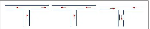
[image:1.612.324.569.476.524.2]Figure (1) shows a schematic representation of the flow distribution through pipe and a general physical setup. Fluid enters the pipe at one end and exit from the other in axial direction .To analyze the fundamental system properties and flow patterns, a simplified flow model was employed in this study. It represents the pipe flow situation as the flow in a straight pipe i.e. main pipe in horizontal direction with one vertical pipe i.e. branch pipe which is connected with the main pipe y an angle of .
Fig. 1: Various possibilities of fluid entering and leaving the junction.
3.
Governing Equations
© 2017, IRJET | Impact Factor value: 5.181 | ISO 9001:2008 Certified Journal | Page 907 ∂u/∂x+∂v/∂y+∂w/∂z=
Navier-Stokes (NS) equation derived by considering three directions of flow x,y and z
{ρ∂u/∂t+ ρu∂u/∂x+ ρv∂u/∂y+ ρw∂u/∂z}∆x∆y∆z = ∑ Fx
Similar equations can be written for y and z
directions.
4. EXPERIMENTAL SET-UP
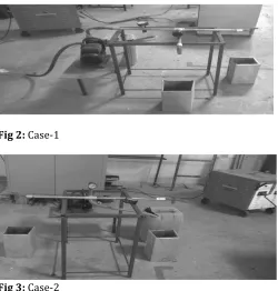
[image:2.612.38.288.314.576.2]The test facility consists of G.I pipes of 0.2 m diameter and 1m length as shown in the figure 2 below. Water is used as working fluid; pressure gauge is used for pressure measurement, centrifugal pump (0.5Hp) is used for supply of fluid. Two cases are considered in first case one outlet is considered at 900 and another at 1800.
Fig 2: Case-1
Fig 3: Case-2
AS shown in figure 3 both the outlets are at 900 with respect to inlet. Water is allowed to pass through inlet and discharge is measured.
4.2 Experimental Results
For the first case in which both the outlets are at different angle are as follows. In first case angle between inlet and ontlet-1 is 1800 and for second outlet it is 900. In second case angle for both the outlets is 900 with respect to inlet.
Table 1 : Experimental results for case-1
Table 2: Experimental results for case-2
Both the results obtained above by changing the inlets, this result are to be used for CFD analysis.
5. Computational Fluid Dynamics
Computational fluid dynamics, usually abbreviated as CFD, is a branch of fluid mechanics that uses numerical analysis and algorithms to solve and analyze problems that involve fluid flows. Computers are used to perform the calculations required to simulate the interaction of liquids and gases with surfaces defined by boundary conditions. The Navier–Stokes equations are fundamental basis of almost all CFD problems.
5.1 GAMBIT and FLUENT
Gambit is used as pre-Processor and Fluent is used as post processor. Fluent is the general name for the collection of Computational Fluid Dynamics (CFD) programs sold by Fluent, Inc. of Lebanon, NH. The Mechanical Engineering Department at Penn State has a site license for Fluent, along with its family of programs. Gambit is the program used to generate the grid or mesh for the CFD solver.
Inlet/Outlet Velocity(m/s) Pressure (N/m2) All losses (hf + hi + hb)
Inlet 1.99 0.35
0.59 m
Outlet at 900 0.907 0.306
Outlet at 1800 1.08 0.304
Inlet/Outlet Velocity(m/s) Pressure (N/m2) All losses (hf + hi + hb)
Inlet 1.989 0.4
0.67 m
Outlet at 900 0.993 0.32
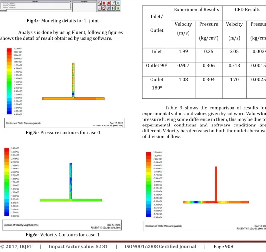
© 2017, IRJET | Impact Factor value: 5.181 | ISO 9001:2008 Certified Journal | Page 908 Fig 4:- Modeling details for T-joint
Analysis is done by using Fluent, following figures shows the detail of result obtained by using software.
Fig 5:- Pressure contours for case-1
Fig 6:- Velocity Contours for case-1
The figure 5 and 6 shows the various Contours of Pressure and velocity of pipe having t-junction with one inlet and two outlets. The color contours shows how the pressure gets increases at the connecting branch of pipe due to which pressure loss occurred in pipe. Same is the case for velocity the Velocity gets increases at the inlet of pipe and decreases in the connecting branch. If we observe the experimental readings it will show same pattern for both cases. We can compare the results.
Table3:- Comparison of experimental and software result.
Inlet/
Outlet
Experimental Results CFD Results
Velocity (m/s)
Pressure
(kg/cm2)
Velocity
(m/s)
Pressure
(kg/cm2)
Inlet 1.99 0.35 2.05 0.0039
Outlet 900 0.907 0.306 0.513 0.00152
Outlet 1800
1.08 0.304 1.70 0.00254
© 2017, IRJET | Impact Factor value: 5.181 | ISO 9001:2008 Certified Journal | Page 909 Fig 7:- Pressure contours for case-2
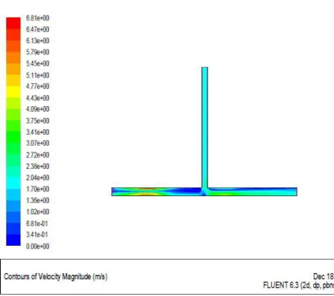
Fig 8:- Velocity Contours for Case-2
[image:4.612.25.571.489.733.2]The above figure 7 and 8 shows the various Contours of Pressure and velocity of pipe having t-junction with one inlet and two outlets, both at 900 with respect to inlet. The color contours shows how the pressure gets increases at the inlet of pipe due to which pressure loss occurred in pipe. The Velocity gets increases at the inlet of pipe and decrease in the connecting branches. Both experimental and software results can be compared as follows.
Table 4:- Comparison of experimental and software result.
Inlet/Outlet
Experimental Results CFD Results
Velocity (m/s)
Pressure
(kg/cm2)
Velocit y
(m/s)
Pressure
(kg/cm2 )
Inlet 1.98 0.4 2.05 0.0296
Outlet 900 0.993 0.32 1.36 0.0185
Outlet 1800 0.967 0.35 1.20 0.0162
Table 4 shows the comparison of results for experimental values and values given by software. Values for pressure are found decreasing in both cases, so we can say that changing angle and division of flow affects flow parameters. Velocity drop is also there due to same factors as that of pressure.
6. Effect of change in angle on T-junction
Recently computational fluid dynamics has been executed to investigate the transition boundaries of different flow patterns for oil-water mixing phenomena. Water lubrication technique is used to reduce the friction during the flow in pipelines of highly viscous oils. Classical formulas such as continuity equation, momentum equation all these equations are solved by volume of flow (VOF) method in fluent. Y-shaped fitting is also found in many pipelines. Work on CFD analysis of Y-shaped branched pipe, including the effect of angle of turn or bend on it is carried out. To study the effect of angle only, Prof. Balvainder Singh and Prof. Harpreet Singh in their work considered all the three pipe branches if 1 inch internal diameter. After studying the effect of bend angle, pipe diameter, pipe length Reynolds number on resistance coefficient. .They come to the conclusion that resistance coefficient vary with change in flow parameters. In CFD analysis of Y-shape joint three angles of 600, 900 and 1800 are selected. But in some cases it may not be possible to use angle of 450 for the flow transmission, so there is scope of improvement by slightly changing the angle from 900. If we reduce the angle to 800 following results shows that losses has been reduced.
Fig. 9 :
Case-1 pressure contours for reduced angle© 2017, IRJET | Impact Factor value: 5.181 | ISO 9001:2008 Certified Journal | Page 910 compared to 900 angles new angle shows pressure drop is
[image:5.612.320.574.76.249.2]reduced.
[image:5.612.38.285.404.556.2]Fig. 10:
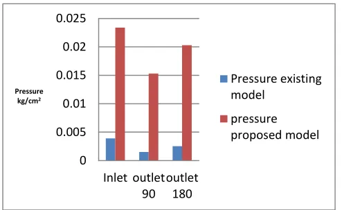
Case-1 velocity contours for reduced angle.Figure.10 shows improved results for velocity of flow through branched pipe.CFD results for existing model and proposed model are compared graphically.
0 0.005 0.01 0.015 0.02 0.025
Inlet outlet 90
outlet 180 Pressure
kg/cm2
Pressure existing model
pressure proposed model
Graph:1
Pressure Comparison Case-1
Graph-1 shows improvement in the values of pressure in all three branches of pipe. Graph-2 Shows With slight change in angle from 900 better results are seen, this will work in overall improvement of results. Similar graphs can be made for second case.
Graph:2
Velocity Comparison Case-1.
7. Future Scope
1. In this study, work was restricted to only water at room temperature and for T-junction joint of pipe. There can be more work done to generalize these results for the other fluids and other junction.
2. With software our ambition is to construct a real time simulation of flow through T- joint of pipe with different inlets. Though this is a very lengthy process, since fluent takes too much time with dynamic mesh, but this is possible with higher versions of fluent and other CFD packages.
3.
In this work we only consider only t-joint in piping system, this kind of work can also be performed for other bends and joints connecting pipes.4.
During this study, we also came across an industrial problem concerning to flow of fluid in pipes. Such kind of problems can be solved with similar techniques.8. Conclusion
© 2017, IRJET | Impact Factor value: 5.181 | ISO 9001:2008 Certified Journal | Page 911 900 angle head loss is minimum if we change the angle, the
energy loss can be decreased by decreasing the angle of t-joint of pipe. From this project after experiment values and Software validation it can be concluded that t-joint dividing flow plays important role in energy loss.
Referances
[1] Anand B. Desamala, “CFD Simulation and Validation of Flow Pattern Transition Boundaries during Moderately Viscous Oil-Water Two-Phase Flow through Horizontal Pipeline”, World Academy of Science, Engineering and Technology, 73 2013. [2] Aslam A. Hirani, C. Udaya Kiran, “CFD Simulation and
Analysis of Fluid Flow Parameters within a Y-Shaped Branched Pipe”, IOSR Journal of Mechanical and Civil Engineering (IOSR-JMCE) e-ISSN: 2278-1684, p-ISSN: 2320-334X, Volume 10, Issue 1 (Nov. - Dec. 2013), PP 31-34.
[3] Boris Hu er, “CFD simulation of a T-junction”, Institute of Hydraulic and Water Resources Engineering, Department of Hydraulic Engineering, Vienna University of technology, Austria.
[4] D. Bhandari and Dr. S. Singh, “Analysis Of Fully Developed Turbulent Flow In A Pipe Using Computational Fluid Dynamics”, International Journal of Engineering Research & Technology (IJERT) Vol. 1 Issue 5, July - 2012 ISSN: 2278-0181.
[5] Gyorgy Paal, Fernando T Pinho and Rodrigo Maia, “Numerical Predictions Of Turbulent Flow In A 90° Tee Junction”The 12th International Conference on Fluid Flow Technologies Budapest, Hungary, September 3 - 6, 2003.
[6] Hiroshi Ogawa, “Experimental Study on Fluid Mixing Phenomena In T-Pipe Junction with Upstream El ow”, The 11th International Topical Meeting on Nuclear Reactor Thermal-Hydraulics (NURETH-11) Popes Palace Conference Center, Avignon, France, 2005. [7] Jafar M. Hassan, Wahid S. Mohammed, “CFD
Simulation for Manifold with Tapered longitudinal Section”, International Journal of Emerging Technology and Advanced Engineering (ISSN 2250-2459,ISO 9001:2008Certified Journal, Volume 4, Issue 2, February 2014)
[8] Jaroslav stigler, Roman Klas and Oldich sperka, “Characteristics of the T-junction with the equal diameters of all branches for the variable angle of the adjacent ranch”, EPJ Web of Conferences, 67, 02110 (2014).
[9] Prof. Balvinder Singh, Prof Harpreet Singh “CFD analysis of Fluid Flow Parameters within A Y-Shaped
Branched Pipe”, International Journal of Latest Trends in Engineering and Technology (IJLTET).
[10] Dr. R. K. Bansal, “Fluid Mechanics and Hydraulic Machines”, Sixth Edition 1 7.
[11] H. K. Versteeg and W. Malasekera, “An Introduction to Computional Fluid Dynamics”, The finite volume method, Longman group Ltd. 1995.