Numerical Analysis of Slurry Flow Characteristics through Horizontal
Pipeline using CFD
Shofique Uddin Ahmed
1, Shuvam Mohanty
21,2 M.Tech Student, Dept. Of Thermal Engineering, Amity University, Haryana, India
---***---
Abstract -
Over the decades conveying solid particles through pipelines has been common practice for many industries such as oil and gas, food industries, pharmaceutical, solid handling, power generations etc. in this present study slurry flow characteristics such as solid concentration distribution, velocity distribution and pressure drops for a 4 m long with pipe diameter 54.9 mm has been analyzed. Particle size of 0.125 mm with specific gravity 2.47 has been considered. Granular Eulerian two phase model with dispersed particles and RNG K-epsilon model have been adopted for the simulation. These models are available in CFD software package FLUENT. Non uniform hexagonal structured mesh has been chosen for the computational domain and the mesh has been refined near the boundary wall. Control volume Finite difference method has been used to solve the governing equations through the whole fluid domain. Simulations are conducted at velocity 2 m/s and 5 m/s and efflux concentration 30% and 40% by volume.Key Words: 3D CFD modelling, Eulerian two phase
model, RNG K-epsilon model, concentration
distribution, velocity distribution, pressure drop, slurry pipeline.
1. INTRODUCTION
Over the years solid-liquid slurry flow through pipelines has been encountered in many fields such as industrial engineering, thermal power plants, oil and gas industries. Many thermal power plants use this method of hydraulic transport of solid materials for disposing waste products. In oil and gas industries crude oil is extracted from the ground along with many solid particles. Horizontal and vertical pipelines are used for conveying crude oil along with these solid particles. Hydraulic transport of solid materials has many advantages over conventional way of transport such as less road traffics, low cost, less air pollution etc. in slurry flow process solid particles are mixed with fluid which form slurry and then it is transported through the pipelines. In general slurry flow regimes can be divided into homogeneous, heterogeneous, moving bed and stationary bed. In homogenous flow regime which consists of small solid particles are kept suspended by the turbulence of the carrier fluid. The heterogeneous flow regime that composed of coarse solid particles, which tend to settle at the bottom of the pipe. The moving bed regime occurs when the solid particles are settled at the bottom of the pipe and tend to move with the flowing fluid along the
pipe forming a bed. The flow rate is considerably slower as the solid bed moves much slower than the flowing fluid. Eventually the solid particles fill the pipe and no further motion is possible and this regime transforms to a stationary bed regime, which is analogous to the flow through a porous medium. The following figures show different types of flow regimes. Among all these flow regimes the most occurring heterogeneous flow regime because no flow regime can be perfectly homogenous.
To understand the whole slurry flow process it is essential to have an accurate prediction of slurry flow characteristics. The effect of solid particle concentrations, velocity distributions and pressure drops along with other flow parameters needs to be studied thoroughly. Many empirical models have been developed over the years to study the slurry flow regime governing mechanisms. CFD (Computational Fluid Dynamics) is a sophisticated computer based numerical analysis system. CFD provides the platform for analyzing complex solid-liquid slurry flow problems by developing and adopting a suitable mathematical model. It helps the researcher conducting a detailed numerical analysis of the flow problem with greater ease and at low cost and also provides extensive information about the local variation of the flow parameters within the computational domain. Researchers over the years have investigated experimentally and numerically solid-liquid slurry flow through both horizontal and vertical pipelines. Researchers are aiming for developing a general model to describe the characteristics of different flow parameters such as concentration distributions, deposition velocity distributions, pressure drop etc for a better understanding of the slurry flow process. Initial studies in this area includes the study of O’Brien (1933)[1] and Rouse (1937) [2], they predicted concentration distribution in a gravity based open channel slurry flow containing very low solid volumetric concentration by using diffusion model. Since then many researcher like Shook and Daniel (1965)[3], Shook et al. (1968)[4], Karabelas (1977)[5], Seshadri et al. (1982)[6], Roco and Shook (1983)[8], Roco and Shook (1984)[9], Gillies et al. (1991)[10], Gillies and Shook (1994)[11], Gillies et al.
(1991)[10], Sundqvist et al. (1996)[16], Mishra et al. (1998)[17], Ghanta and Purohit (1999)[18], Wilson et al. (2002)[19] etc. Apart from these some studies on the prediction of pressure drop in a slurry flow process have been conducted by many researchers. Some of the works in this area includes the work of Masayuki Toda et. al (1971)[20], investigated experimentally the pressure drop in a pipe bend for the solid-fluid slurry flow. Turian and Yuan (1977)[21] developed a pressure drop correlation for flow of slurries in pipelines considering stationary bed, saltation flow, heterogeneous flow and homogenous flow regime. P. Doron et. al (1987)[22] developed a two layer model for the prediction of pressure drop for a slurry flow of coarse particles through horizontal pipelines. The work of Geldart and Ling (1990)[23], Gillis et. al (1991)[10], Doron and Barnea (1995)[24], A. Mukhtar et. al (1995)[25], Turian et. al (1998)[26], J. Bellus et. al (2002)[27] used different models for the slurry flow through pipelines and predicted the pressure drop along with other flow parameters such as concentration distribution, velocity distributions, granular pressure effects, turbulent kinetic energy effects etc.
In this present study the aim is to predict the solid concentration distributions, velocity distributions and pressure drop by applying Eulerian two phase model in a 4 m long pipe with pipe diameter of 54.9 mm. solid particles are considered as mono-dispersed and particle size of 0.125 mm mean diameter with specific gravity of 2.47 is considered. The simulations are conducted at velocity 2 m/s and 5 m/s and efflux solid concentration of 30% and 40%.
2. MATHEMATICAL MODEL
The Granular version of Eulerian two phase model has been considered in this present study for modeling the solid-fluid slurry flow. Particles are considered as mono dispersed. RNG K-epsilon model has been used for modeling the turbulent flow.
2.1 Eulerian model:
Eulerian model assumes that the slurry flow consists of solid ‘‘s’’ and fluid ‘‘f’’ phases, which are separate, yet they form interpenetrating continuum, so that
,
, where αf and αs are the
volumetric concentrations of fluid and solid phase, respectively.The laws for the conservation of mass and momentum are satisfied by each phase individually
.
2.1 Governing Equations
1. Continuity Equation:
⃗
2. Momentum Equation for fluid phase:
(
⃗
⃗
)
̿
⃗
(
⃗⃗⃗⃗
⃗⃗⃗⃗)
⃗⃗⃗⃗
⃗⃗⃗⃗
⃗⃗⃗⃗
⃗⃗⃗⃗
( ⃗
⃗
)
⃗⃗⃗⃗
3. Momentum Equations for solid phase:
⃗
⃗
̿
⃗
(
⃗⃗⃗⃗
⃗⃗⃗⃗)
(
⃗⃗⃗⃗
⃗⃗⃗⃗
⃗⃗⃗⃗
⃗⃗⃗⃗)
( ⃗
⃗
)
⃗⃗⃗⃗
Where
̿
and̿
are the stress tensors for solid and fluid respectively.4. Turbulent Equation:
̿̿̿̿ ( ⃗) ̿ ⃗ ⃗
Here is the turbulent viscosity. RNG theory provides
an analytically-derived differential correlation for turbulent viscosity that accounts for low Reynolds number effects. This correlation in the high Reynolds number limit (as the cases in present study) converts to:
With
The predictions of turbulent kinetic energy and its rate of dissipation in RNG k-ε model are similar to Standard
k-ε model, described widely in published researches on CFD. The main difference between the RNG and standard
k-ε models lies in the additional term in the ε equation given by:
Where, , , , the constant
parameters used in the different equations are taken
as , , , ,
5. Wall functions:
Near wall boundary regions need special treatments for accurate perdition of flow parameter behaviour near the wall. This is achieved by using standard wall functions available in the RNG K-epsilon model.
3. NUMERICAL SOLUTION
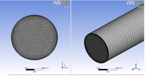
3.1 Geometry and mesh
with smooth transition are used for meshing the computational domain. Inflation layers allow refined mesh near the wall boundary region. There are approximately 382004 elements in the mesh. (Fig. 1).
Fig -1: View of mesh used in this study.
3.2 Boundary Conditions
Three boundary conditions for the flow domain are introduced namely inlet boundary, wall boundary and outlet boundary. Velocity and efflux solid concentrations have been introduced to the inlet boundary. No slip boundary conditions are applied for wall and pressure outlet boundary condition has been introduced for outlet boundary. A fully developed flow at outlet is used for concentration and velocity profiles.
3.3 Solution Strategy
Second order upwind discretization scheme is used for momentum equation, turbulent kinetic energy and turbulent dissipation energy, first order discretization scheme is used for volume fraction. Pressure and velocity coupling phase coupled SIMPLE algorithm is used for multiphase flow. The under relaxation factors (URF) for momentum and volume fraction is reduced from 0.7 to 0.5 and 0.5 to 0.3 respectively. This combination ensures satisfactory accuracy, stability and convergence of the problem.
4. RESULTS AND DISCUSSIONS
4.1 Concentration distributions
Fig. 2 to 6 show the simulated contours of volumetric concentration of the solid particles along vertical centerline of the cross section of pipe outlet. Here
is predicted concentration of the solid particles along the cross section of pipe outlet, is local volumetric
concentration of the solid particles.
,
Y being the height of vertical centreline from top to bottom of the pipe cross section in y-direction.(a) V= 2m/s
(b) V= 5m/s
Fig-2: Solid concnetration distribution predicted at
[image:3.595.40.283.139.268.2]
(b) V= 5 m/s
Fig-3: Solid concnetration distribution predicted at
4
(a) V= 2m/s (b) V= 5m/s
Fig-4: plots of predicted solid concentration at
(a) V= 2 m/s (b) V= 5m/s
Fig-5: plots of predicted solid concentration at
It can be observed from Fig. 2 to 5 that the distribution of solid particles is asymmetrical along the vertical plane of the pipe outlet. The higher concentration zone is at the lower half of the pipe where the solid particles tend to settle down at the bottom of the pipe due to gravitational effect. This is observed at lower velocity say V=2 m/s. it is also observed that the asymmetry of the solid particle distribution decreases at a given efflux concentration
pipe. This happens because as velocity increases, the turbulent energy increases which allow the solid particles to mix properly with the fluid. It is also observed that the interaction of solid particles with the pipe wall increases at higher efflux concentration and higher velocity.
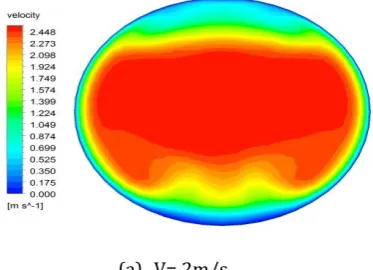
4.2 Velocity distributions
Fig.6 to 11 show the velocity distributions at efflux concentration level of 30% and 40% respectively. The velocity contours are obtained at outlet of the pipe.
[image:4.595.37.281.72.446.2](a) V= 2m/s
Fig-6: Simulated velocity distribution at
[image:4.595.63.262.83.240.2]
(b) V= 5m/s
Fig-7: Simulated velocity distribution at
(C) V= 2m/s
Fig-8: Simulated velocity distribution at
-0.5 -0.3 -0.1 0.1 0.3 0.5
0 1 2 3
Y'
C(Y')/Cvf
-0.5 -0.3 -0.1 0.1 0.3 0.5
0 1 2
Y'
C(Y')/Cvf
-0.5 -0.3 -0.1 0.1 0.3 0.5
0 1 2
Y'
C(y')/Cvf
-0.5 -0.3 -0.1 0.1 0.3 0.5
0 0.5 1 1.5
Y'
[image:4.595.340.527.226.361.2] [image:4.595.38.280.468.625.2] [image:4.595.338.530.596.738.2]V= 5m/s
Fig-9: Simulated velocity distribution at
(a) V= 2m/s
(b) V= 5m/s
Fig-10: Plots of simulated velocity distribution at
(a) V= 2m/s
(b) V= 5m/s
Fig-11: Plots of simulated velocity distribution at
From Fig. 6 to 11 it can be observed that the velocity distribution is parabolic an asymmetrical at the lower portion of the pipe. This asymmetrical nature of velocity distribution is more at low velocity say V= 2m/s this is due to the larger shear force as the particles settle down at the bottom of the pipe. However when velocity increases at given efflux concentration the velocity distributions become more symmetrical. It can also be observed that at any given velocity as the efflux concentration increases the asymmetrical nature of velocity distribution also increases.
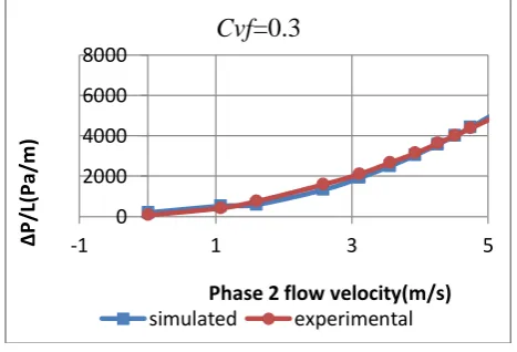
4.3 Pressure drop
[image:5.595.37.559.27.822.2]The effect of solid concentrations and solid particles flow velocity on pressure drop is analyzed in this section. The predicted simulated results of pressure drop have been validated with experimental data available in previous literature [28]. Differential pressure along the length (ΔP/L) is taken on Y-axis and phases 2 flow velocity of the solid particles is been taken on X-axis for plotting the graphs.
Fig-12: Comparison of simulated and experimental pressure gradient over phase 2 flow velocity at different
velocities and
-0.5 -0.3 -0.1 0.1 0.3 0.5
0 1 2 3
Y'
=Y/
D
flow velocity of solid particles
-0.5 -0.3 -0.1 0.1 0.3 0.5
0 2 4 6
Y'
=Y/
D
flow velocity of solid particles
-0.5 -0.3 -0.1 0.1 0.3 0.5
0 1 2 3
Y'
=Y/
D
flow velocity of solid particles (m/s)
-0.5 -0.3 -0.1 0.1 0.3 0.5
0 2 4 6 8
Y'
=Y/
D
flow velocity of solid particles (m/s)
0 2000 4000 6000 8000
-1 1 3 5
ΔP
/L
(P
a/
m
)
Phase 2 flow velocity(m/s)
Cvf
=0.3
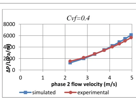
[image:5.595.319.553.568.727.2]Fig-13: Comparison of simulated and experimental pressure gradient over phase 2 flow velocity at different
velocities and
From Fig.12 and 13 the development of pressure drop with an increase in velocity can be observed and increase in flow velocity leads to increase in pressure drop. It can also be observed that at a given velocity, the rate of increase in pressure drop is less at lower efflux and the rate increases rapidly at higher efflux concentrations.
5. CONCLUSIONS
Based on the simulated results the following conclusions can be drawn:
The solid particle distributions are asymmetrical along the vertical plane of the pipe cross section.
At low velocities the higher concentration zone is at the lower portion of the pipe, particles tend to settle at the bottom of the pipe.
The asymmetrical nature of the particles distributions decreases for higher velocities where particles are lifted from the bottom of the pipe under the influence higher of turbulent energy.
The particles interaction with pipe wall becomes more vivid at higher velocities.
Velocity distributions are parabolic and asymmetrical at the lower portion of the pipe.
For a given efflux concentration velocity distributions become more symmetric at higher velocities.
The asymmetrical nature of velocity distribution increases at higher efflux concentration at a given velocity.
Pressure drop increases with increase in flow
For a given velocity at lower concentration the rate of increase in pressure drop is less and at higher concentrations the rate increases rapidly and abruptly.
REFERENCES
[1] O’Brien, M.P., 1933. Review of the theory of
turbulent flow and its relations to sediment transport. Transaction of the American Geophysical Union 14, 487–491.
[2] Rouse, H., 1937. Modern conceptions of the
mechanics of fluid turbulence. Transactions of ASCE, 102, 463–505.
[3] Shook, C.A., Daniel, S.M., 1965. Flow of
suspensions of solids in pipeline: I. Flow with a stable stationary deposit. The Canadian Journal of Chemical Engineering, 43, 56–72.
[4] Shook, C.A., Daniel, S.M., Scott, J.A., Holgate, J.P.,
1968. Flow of suspensions in pipelines. The Canadian Journal of Chemical Engineering, 46, 238–244.
[5] Karabelas, A.J., 1977. Vertical distribution of
dilute suspensions in turbulent pipe flow. AIChE Journal, 23, 426–434
.
[6] Seshadri, V., 1982. Basic process design for a
slurry pipeline. In: Proc. The Short Term Course on Design of pipelines for transporting liquid and solid materials, IIT, Delhi.
[7] Seshadri, V., Malhotra, R.C., Sundar, K.S., 1982.
Concentration and size distribution of solids in a slurry pipeline. In: Proc. 11th Nat. Conference on Fluid mechanics and fluid power, B.H.E.L., Hyderabad.
[8] Roco, M.C., Shook, C.A., 1983. Modeling of slurry
flow: The effect of particle size. The Canadian Journal of Chemical Engineering, 61, 494–503.
[9] Roco, M.C., Shook, C.A., 1984. Computational
methods for coal slurry pipeline with heterogeneous size distribution. Powder Technology, 39, 159–176.
[10] Gillies, R.G., Shook, C.A., Wilson, K.C., 1991. An
improved two layer model for horizontal slurry pipeline flow. The Canadian Journal of Chemical Engineering, 69, 173–178.
[11] Gillies, R.G., Shook, C.A., Wilson, K.C., 1991. An
improved two layer model for horizontal slurry pipeline flow. The Canadian Journal of Chemical
0 2000 4000 6000 8000
0 1 2 3 4 5
ΔP
/L
(P
a/
m
)
phase 2 flow velocity (m/s)
Cvf=0.4
[12] Gillies, R.G., Hill, K.B., Mckibben, M.J., Shook, C.A.,
1999. Solids transport by laminar Newtonian flows. Powder Technology, 104, 269–277.
[13] Gillies, R.G., Shook, C.A., 2000. Modeling high
concentration settling slurry flows. The Canadian Journal of Chemical Engineering, 78, 709–716.
[14] Wasp, E.J., Aude, T.C., Kenny, J.P., Seiter, R.H.,
Jacques, R.B., 1970. Deposition velocities, transition velocities and spatial distribution of solids in slurry pipelines. In: Proc. Hydro transport 1, BHRA Fluid Engineering, Coventry, UK, paper H4.2, pp. 53–76.
[15] Doron, P., Granica, D., Barnea, D., 1987. Slurry
flow in horizontal pipes-experimental and modeling. International Journal of Multiphase Flow, 13, 535–547.
[16] Sundqvist, A., Sellgren, A., Addie, G., 1996. Slurry
pipeline friction losses for coarse and high density products. Powder Technology, 89, 19–28.
[17] Mishra, R., Singh, S.N., Seshadri, V., 1998.
Improved model for prediction of pressure drop and velocity field in multisized particulate slurry flow through horizontal pipes. Powder Handling and Processing Journal, 10, 279–289.
[18] Ghanta, K.C., Purohit, N.K., 1999. Pressure drop
prediction in hydraulic transport of bi-dispersed particles of coal and copper ore in pipeline. The Canadian Journal of Chemical Engineering, 77, 127–131.
[19] Wilson, K.C., Clift, R., Sellgren, A., 2002. Operating
points for pipelines carrying concentrated heterogeneous slurries. Powder Technology, 123, 19–24.
[20] Toda, M., Komori, N., Saito, S., & Maeda, S. (1972).
Hydraulic conveying of solids through pipe bends. Journal of Chemical Engineering of Japan, 5(1), 4-13.
[21] Turian, R. M., & Yuan, T. F. (1977). Flow of
slurries in pipelines. AIChE Journal, 23(3), 232-243.
[22] Doron, P., Granica, D., & Barnea, D. (1987). Slurry
flow in horizontal pipes—experimental and modeling. International Journal of Multiphase Flow, 13(4), 535-547.
[23] Geldart, D., & Ling, S. J. (1990). Dense phase
conveying of fine coal at high total pressures. Powder Technology, 62(3), 243-252.
[24] Doron, P., & Barnea, D. (1995). Pressure drop and
limit deposit velocity for solid-liquid flow in pipes. Chemical engineering science, 50(10), 1595-1604.
[25] Mukhtar, A., Singh, S. N., & Seshadri, V. (1995).
Pressure drop in a long radius 90° horizontal bend for the flow of multisized heterogeneous slurries. International journal of multiphase flow, 21(2), 329-334.
[26] Turian, R. M., Ma, T. W., Hsu, F. L. G., & Sung, D. J.
(1998). Flow of concentrated non-Newtonian slurries: 1. Friction losses in laminar, turbulent
and transition flow through straight
pipe. International journal of Multiphase
flow, 24(2), 225-242.
[27] Bellas, J., Chaer, I., & Tassou, S. A. (2002). Heat
transfer and pressure drop of ice slurries in plate
heat exchangers. Applied Thermal
Engineering, 22(7) ,721-732.
[28] Kaushal, D.R., & Tomita, Y. (2007). Experimental