Reduced Partition Function Ratio in the Frequency Complex Plane: A Mathematical Approach

http://dx.doi.org/10.4236/ojg.2014.412049

How to cite this paper: Yuan, J. (2014) Reduced Partition Function Ratio in the Frequency Complex Plane: A Mathematical Approach. Open Journal of Geology, 4, 654-664. http://dx.doi.org/10.4236/ojg.2014.412049

Reduced Partition Function Ratio in

the Frequency Complex Plane:

A Mathematical Approach

Jie Yuan

Key Laboratory of Earth and Planetary Physics, Institute of Geology and Geophysics, Chinese Academy of Sciences, Beijing, China

Email: [email protected]

Received 25 September 2014; revised 20 October 2014; accepted 18 November 2014

Copyright © 2014 by author and Scientific Research Publishing Inc.

This work is licensed under the Creative Commons Attribution International License (CC BY). http://creativecommons.org/licenses/by/4.0/

Abstract

This paper gives a mathematical approach to calculate the fractionation factor of isotopes in a general cluster (also known as super-molecule), which composes of necessary chemical effect within three bonds outside the interested atom(s). The cluster might have imaginary frequencies after being optimized in quantum softwares. The approach includes the contribution of the dif-ference, which is resulted from the substitution of heavy and light isotopes in the cluster, of vibra-tions of imaginary frequencies to give precise prediction of isotope fractionation factor. We call the new mathematical approximation “reduced partition function ratio in the frequency complex plane (RPFRC)”. If there is no imaginary frequency for a cluster, RPFRC is simplified to be Urey (1947) or Bigeleisen and Mayer (1947) formula. Final results of this new algorithm are in good agreement with those in earlier studies.

Keywords

Isotope Fractionation, Cluster, Reduced Partition Function Ratio, Frequency Complex Plane

1. Introduction

In 1933, Urey and Rittenberg [1] pointed out that the isotopic fractionation factor in different systems could be calculated from spectroscopic data. A more convenient method for the calculation is known as Urey (1947) [2]

655

vibrational frequencies [4], RPFR cannot evaluate the isotope fractionation factor since it does not deal with imaginary frequencies (see details in Section 2.2).

To overcome this difficulty, Rustad et al. (2008) [4] applied the partial Hessian vibrational analysis (PHVA)

[5] in the carbonate (e.g., calcite, aragonite and magnesite) clusters to predict the distributions of isotopes in these minerals; this operation neglects all imaginary frequencies (as well as some real ones) and then the re-mainder of real frequencies in the sets are used in RPFR, giving the carbon isotope fractionation factors in these minerals. But when using PHVA, also neglected is the contribution of the differences (due to the substitution of heavy and light isotopes in clusters) of imaginary frequencies to the isotope fractionation effect [6]. Therefore, previous problem is still under debate.

This study gives a new approach, i.e. reduced partition function ratio in the frequency complex plane (RPFRC),

to the calculation of isotope fractionations in general clusters. This new approach involves a more detailed physical figure of atom vibrations for the calculation than PHVA did; that is, the vibrations of all atoms due to the substitution of heavy and light isotopes in clusters are included to predict the isotope fractionations. This new approach is finally tested by studying isotope fractionation factors in liquid and mineral phases.

2. Theory

2.1. General Cluster for Isotope Research

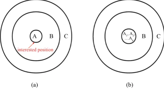
We firstly give the theoretical background on building a general cluster for isotope research. The general cluster (Figure 1) includes three parts: A) interested isotopic atom(s) of an element at specific position; B) atoms link-ing three chemical bonds outside the interested atom(s). Stern and Wolfsberg (1966) [7] had theoretically proved that the biggest necessary influence of chemical effects on an interested isotope is within three bonds; and C) atoms to make the system to be converged in softwares. This kind of cluster could model isotope fractionations in both liquid and solid phases. In practical, researchers cut off atoms from a large periodical system to form solid-phase (e.g., calcite and aragonite in Ref. [4]) clusters, and terminate the outside-broken bonds in part B

with some hydrogen atoms in part C. For liquid phase, one adds few water molecules (and sometimes few ions

[8]) around the interested isotope to simulate its water environments; this technique is also called as “wa-ter-droplet” method [4] [9] [10]. For convenience, we represent the general cluster as a super-molecule XAp, where A and X represent the interested atom and all atoms in parts of both B and C respectively and the subscript

p the number of interested atoms of the same element in the center of the cluster (Figure 1(b)).

2.2. Harmonic Frequencies in Complex Plane

As discussed above, the super-molecule is sufficient to describe the chemical influence on isotopes at interested position; then one can use ab initio molecular orbital theory to get the frequencies. In Ref. [11], mass-weighted

Figure 1. (a) 2-D schematic diagram of general cluster/super-molecule XA

[image:2.595.163.433.513.662.2]

656 force constants are defined by

1 2 1 2

jk jk j k

f′ = f m− m− (1)

where mk is the mass of the kth atom in the molecule, and the force-constant fjk is the second energy deriva-tives for coordinates Rj and Rk._. And the kth normal-mode displacements has the form

(

)

exp 2π

k k

r =a vit (2)

where

2 2

4π

jk j k

j

f a′ = ώ a

∑

(3)

in which 4π2v2 are the eigenvalues of the matrix fjk′, and ώ are the harmonic frequencies (Hz). This equa-tion gives one set of frequencies for the heavy-isotope system and another for the light-isotope system; these two sets of frequencies are used to calculate the isotope fractionation factor.

The two sets of harmonic frequencies for a super-molecule would, however, sometimes have imaginary fre-quencies [12]. This is due to the fact that one cannot find a local minimal on the potential energy surface for all atoms of the cluster. And there will be some minus force constants in Equation (1). Upon taking the square root of the left hand side of Equation (3) for a minus mass-weighted force constant, a factor of complex unit i will emerge, and there will be some imaginary frequencies for the molecule. Under this case, one cannot use RPFR to calculate the distribution of isotopes in the super-molecule, because only real frequencies are suitable for RPFR.

For a super-molecule, we suggest that all frequencies, especially the imaginary ones, should be included in the calculation of isotope fractionation. The reasons come from the following facts [11]: for a random frequency

k

ώ , Equations (2) and (3) give the displacement (ak and aj) of each and every atom in the cluster. In other

words, it gives a very important physical figure: all atoms in cluster will have a motion (with amplitude aj) for frequency ώk. From this point of view, even an imaginary frequency has motions of all atoms in the molecule, and it will affect the difference of the isotope fractionation as vibrational contribution (see the next subsection).

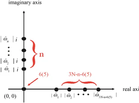
In mathematics [13], each set of frequencies has characteristic properties. The frequencies can be plotted on the complex plane (Figure 2), which is a geometric representation of the complex numbers established by the real axis and the orthogonal imaginary axis. For a general super-molecule, the eigenvalues of the mass-weighted matrix will have 3N frequencies, which might include n imaginary ones, 6 (5) (6, for nonlinear molecular, 5, for linear and diatom molecular) zeros (corresponding to translations and rotations), and 3N− −n 6 5

( )

real ones. All non-zero frequencies locate on those two axes, and the zeros at the origin. A real frequency equals its ownmodulus, i.e. ώreal= ώreal ; and an imaginary one equals its own modulus multiplying the unit of complex

number, i.e. ώimaginary = ώimaginary i.

Figure 2.Plots of frequencies for one cluster/super-molecule on

[image:3.595.179.412.522.695.2]

657

2.3. Evaluation of Partition Function and Free Energy of the Super-Molecule

Based on the Born-Oppenheimer approximation (i.e. nearly harmonic approximation) [14], the translational and rotational, and vibrational energies are the main contribution to the difference of isotope exchange reactions [2] [3]. The followings discuss the partition functions of these three kinds of energies and give the total free energy for the super-molecule.

The translational and rotational energies are in the form of

2 2 2 2

2 2 2

8 y x z trans n n n h E

M a b c

 

= _ + + _

 

(

nx y z, , =1, 2,

)

and

(

)

2 2 1 8π rot

h J J E

I

+

=

(

J =0,1, 2,

)

[15], which are all real numbers. So the translational partition function for

the super-molecule is

3 2 2 2π b trans Mk T Q V h  

= _ _ (4)

where V is the volume of the cluster, M is the mass of the cluster, kb is the Boltzmann constant, T is the absolute temperature, h is the Plank constant. And the rotational partition function is

2 2 8π b rot Ik T Q h σ

= (5)

for diatomic and linear molecules

(

)

3 2

(

)

1 2 1 2 2

3

π 8π b A B C rot

k T I I I

Q

h

σ

= (6)

for nonlinear molecules, where σ is the symmetry number of the molecule, and IA is the moment of inertia with respect to the appropriate principal axis.

The vibrational energy is in the form of

1

1 2 n

vib k i

k

E hώ υ

=

 

= _ + _

 

∑

(each υ =i 0,1, 2,); but the imaginary fre- quencies cannot be included in this expression and the partition function in the classical mechanism [15]. How-ever, as shown in previous subsection, this study needs to introduce the contribution of all imaginary frequencies into the partition function and free energy to calculate the isotope fractionation factor. Thus, only for isotope re-search in ab initio studies, we suggest the vibrational partition function of the super-molecule to be

( )

3 6 5 2 1 e 1 e k b k b hc

N k T

vib _hc k k T Q ω ω − − ∗ − = −

=

_∏



 (7)

where ώk is the modulus of the kth frequency from Equation (3). If ώk is real, Qvib k ∗

is the vibrational par-tition function; and if ώk is imaginary, Qvib k

∗

is defined as imaginary-frequency correction to the vibrational partition function. Thus we call Qvib

∗

the imaginary-frequency-corrected vibrational partition function. Fur-thermore, the imaginary-frequency-corrected Helmholtz free energy of this super-molecule is given by

( )

ln

F∗= −RT Q∗ (8)

where R is gas constant and

trans rot vib

Q∗=Q Q Q∗ (9)

2.4. Teller-Redlich Product Rule in the Frequency Complex Plane

In Ref. [16], Equation (3) can also be expressed as

[ ] [ ]

FG F µ µ1 2 µN λ λ1 2 λN

∗

658

where

[ ]

G is the kinetic energy matrix, µk is the reciprocal mass of the kth atom in the molecule,

[ ]

F is the force-constant matrix, and

2 2 2 2 2

4π 4π

k vk c k

λ = = ω (11)

Since

[ ]

F will be identical for the molecule of different isotopes with the same method (i.e. the same ex-change-correlation functional/basis set), now taking Equation (11) into Equation (10) gives

1 2 1 3 1 2 3 1 3 1 2 3

N N

N N

m m m

m m m

ω ω ω ω ′ ′   =  _{′ ′ ′}      

   (12)

where the superscript “ ′ ” denotes the molecule with heavy isotopes.

Let us submit the frequencies with complex form. The number n of complex unit i is dependent on left hand side of Equation (3) and right hand side of Equation (1). Because mk, mk′ are real and nearly the same for one element, and the force constant matrix fij is identical for a cluster with given method, n are the same in the numerator and denominator of Equation (12). We get

1 2 1 1 3 1 2 3 1 1 3 1 2 3

k k N N

k k N N

i i m m m

i i m m m

ω ω ω ω

ω ω ω ω

+ + ′ ′ ′ ′   =  _{′ ′ ′}          

       (13)

After the cancellation of i, we have

1 2 1 1 3 1 2 3 1 1 3 1 2 3

k k N N

k k N N

m m m

m m m

ω ω ω ω

ω ω ω ω

+ + ′ ′ ′ ′   =  _{′ ′ ′}          

       (14)

Equation (14) is valid only when 3N motions are vibrational normal modes. We consider those 6 (5) mo-tions, corresponding to translational and rotational momo-tions, convert of low frequency corresponding to weak forces. Then the ratio for the translational frequencies and rotation frequencies can be written as:

1 2 T T M M ω ω ′ _{ } =  _′   

 (15)

1 2 R R I I ω ω ′ _{ } =  _{ ′} 

 (16)

Submitting Equations (15) and (16) into Equation (14), we obtain the Teller-Redlich product rule in the fre-quency complex plane:

1 2 _{3 2} 3 5 3

1 1

N N

k i

k k i i

m M I

m M I

ω ω − = = ′ ₌    ′  ′  _′ _   _{  }  

∏

_

∏

(17a)

for diatom and linear molecules and

1 2 3 2 1 2 3 6 3

1 1

N N

k i A B C

k k i i A B C

m M I I I

m M I I I

ω ω − = = ′ ₌    ′  ′ ′ ′   _′ _ _      

∏

_

∏

(17b)

for nonlinear molecules.

3. Reduced Partition Function Ratio in Frequency Complex Plane

The differences for the isotopes in the super-molecule can be written as a typical chemical exchange reaction [2] [3]:

1 1

p p

XA A XA A

p + ′= p ′ +

659 The equilibrium constant for this reaction is given by

(

)

exp

K = −∆G RT (18)

Because different isotopes have negligible difference of volume, isotope exchange reactions do not involve significant pressure-volume work [15]. The Gibbs free energy is equivalent to the Helmholtz free energy and we take Equation (8) into Equation (18), K can be written as partition function ratio:

( )

( )

( )

( )

1p p p

Q XA Q A

K Q A Q XA ∗ ∗  ′  ′   =     (19)

Let us substitute Equations (5)-(8) into Equation (19). For diatom and linear molecules, we have

( )

( )

( )

_{( )}

( )

_{( )}

( ) ( ) ( ) ( ) 1 1 3 2

3 2 _{2 2}

3 5 _{e e}

1 e 1 e

k p k p

p

k p k p

p

p

u XA u XA

N XA

p p

u XA u XA

k XA

p p

M XA I XA

m A K

m A M XA I XA

σ σ − ′ − − − ′ − − ′ _{ ′  ′    }   _{  }       =_{ ′} _{     }× _{ }  

  _{ }

∏

_ − _{ } − _{ } (20a)

and for nonlinear molecules,

( )

( )

( )

_{( )}

( ) ( ) ( )

_{( ) ( ) ( )}

( ) ( ) ( ) ( ) 1 1 3 2

3 2 _{2 2}

3 6 _{e e}

1 e 1 e

k p k p

p

k p k p

p

p

u XA u XA

N XA

p A p B p C p

u XA u XA

k XA

p A p B p C p

M XA I XA I XA I XA

m A K

m A M XA I XA I XA I XA

σ σ − ′ − − − ′ − − ′ _{ ′  ′ ′ ′    }   _{      }   =_{ ′} _{     }× _{ }  

  _{ }

∏

_ − _{ } − _{ } (20b)

where uk =hcώ k Tk b .

Equation (20) can be reduced to a more general expression by using Equation (17):

( )

( )

( )

( )

( )

{

{

( )

( )

}

}

' 1 3 6 5

C

1 exp

exp 2

RPFR

exp 2 1 exp

p p p N k p k p

XA k p

p

k _{k p k p}

XA k p

u XA u XA

u XA XA

u XA u XA u XA

σ σ −  _{′ − ′  − − }          =   _{ −  − − ′ } _      

∏

(21)

whereRPFRCis short forreduced partition function ratio in the frequency complex plane.

Obviously, one can see that if the super-molecule is at a local minimal on the potential energy surface (i.e. 0

n= ), all frequencies locate on the real-axis in the frequency complex plane (Figure 2). In such case, RPFRC

becomes Urey (1947) or Bigeleisen and Mayer (1947) formula. Due to the fact that the set of real numbers (i.e.

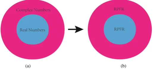
frequencies here) is the subset of the set of the complex numbers [13], the set of fractionation factors given by Urey (1947) or Bigeleisen and Mayer (1947) formula (i.e. RPFR) is the subset of the set of fractionation factors given by Equation (21) (i.e. RPFRC) (Figure 3). In other words, this work extends Urey and Rittenberg’s (1933)

idea [1] to focus on isotope fractionation research in the frequency complex plane. The fractionation factor between two clusters can be written as:

C1 C2

RPFR RPFR

α = (22)

[image:6.595.170.433.547.664.2]

(a) (b)

Figure 3. (a) The set of real numbers (i.e. frequencies here) is a subset of the set of the complex numbers; (b) The set of RFPR is a subset of the set of RPFRC. The arrow indicates the process of the calculation of the isotope

fractionation factors. Using real frequencies and imaginary ones in the

660

4. Tests of Present Approach

To understand the new algorithm, we compute RPFRC and/or α in typical isotope systems. Two examples are

depicted below not for the accuracy prediction of experimental data, butfor the abilities of our algorithm. All frequencies needed in RPFRC are implemented in Gaussian09 [12]. The optimized geometries and frequencies

for all examples are presented in the “Electronic supplementary materials”. Present RPFRC and α results are

compared with corresponding references, i.e. those previously calculated from all real frequencies in published literatures. The difference ε (in ‰) between present result and the reference is in the form of

(

RPFRC RPFRref 1

)

1000

ε = − ∗ or ε=

(

α αref − ∗1

)

1000.

1) The geranium isotope fractionation factor α between GeO OH

( ) (

31- H O2

)

30

−

(Figure 4(a)) and Ge(OH)4-(H2O)30 (Figure 4(b)) (corresponding to

( ) (

)

1 2 3 30

GeO OH − - H O _B and Ge(OH)4-(H2O)30_D in Ref.

[10] respectively) is a good example of study of isotopes in liquid phase. After optimized, each cluster has an imaginary frequency (Table 1). When calculating α, Li et al. (2009) neglected the imaginary frequencies be-cause 1) the main vibration vector of this imaginary frequency belongs to a water molecule located at outside of the super-molecule; 2) it is less than 50 cm−1; and 3) RPFR is the same if they neglected it. The values of Li et al.’s

αs at different temperatures are taken as references. As shown in Figure 5, the maximum difference εmax be-

(a) (b)

Figure 4. Water-droplets for a)

(

) (

1 ₂

)

3 30

GeO OH − - H O , and b) Ge(OH)4-(H2O)30 (cyan

germanium, gray hydrogen, red oxygen). The optimized structures and frequencies are

[image:7.595.127.466.291.429.2]

tak-en from Li et al. (2009).

Figure 5.εα Ge(OH)4-(H2O)30-

(

) (

)

1 2

3 30

GeO OH − - H O versus T(K). The corresponding re-

[image:7.595.181.419.485.689.2]

661

tween Li et al.’s and present results is 8.2 × 10−5‰ (273.15 K); this shows that present approach is very efficient to study isotope fractionation in liquids.

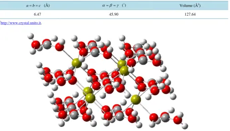
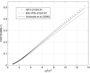
2) The carbon and 13C-18O clumped isotope fractionations in inner body of calcite are good examples of study of isotopes in solid phase. We cut a cluster (Figure 6) from the periodical calcite, of which the primitive cell parameters (Table 2) are calculated in CRYSTAL06 [17], by the way published in Rustad et al. (2008). The fitted polynomials of

3 CaCO -C

α and K3866 in Ref. [18] are taken as references.

Results shown in Figures 7-9 indicate that our new algorithm have high accuracy. For 3 CaCO -C

α in Figure 7,

max

ε s are −10.2‰ (273.15 K) and −4.8‰ (273.15 K) for HF/3-21G/0.91 (the scaling factor) and B3LYP/6- 31G/0.97 [19]-[21] levels, respectively; and the difference of εmaxs between present results and data given by

PHVA in Rustad et al. (2008) are −0.1‰ (=−4.1‰ - (−4‰), 298.15 K) and −3‰ (=−7‰ - (−4‰), 298.15 K)

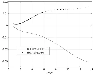
for HF/3-21G/0.91 and B3LYP/6-31G/0.97 levels, respectively. For K3866 in Figure 8 and Figure 9, εmaxs

between present result and data given by Schauble et al. (2006) are 0.015‰ (273.15K) and −0.031‰ (273.15K)

[image:8.595.88.540.293.399.2]

for HF/3-21G/0.91 and B3LYP/6-31G/0.97 levels, respectively. It seems clear that K3866 is not sensitive to the exchange-correlation functional/basis set/scaling factor, the number of imaginary frequency n and the magnitude of the frequencies (shown in Table 1 and the “Electronic supplementary materials”).

Table 1. Methods/basis_sets/scaling factors1 used in Gaussian09 and the results of super-molecules.

Super-molecule Method/Basis_set/Scaling factor

Imaginary Frequency (cm−1)*

n Minimal Maximal

( ) (1 )

2

3 30

GeO OH− - H O B3LYP/6-311+G**/1.052 1 −5.07 −5.07

Ge(OH)4-(H2O)30 B3LYP/6-311+G**/1.052 1 −22.23 −22.23

Calcite cluster HF/3-21G/0.91 76 −7119.47 −11.93

Calcite cluster B3LYP/6-31G/0.97 151 −3321.80 −69.95

1

[image:8.595.88.541.438.697.2]

http://cccbdb.nist.gov/. 2See Ref. [10]. n is the number of imaginary frequency. *The frequencies correspond to molecules with 70Ge, 12C16O.

Table 2. Primitive cell parameter of calcite from CRYSTALL06, with B3LYP/(Ca_86-511d3G, C_6-21Gd, O_8-411d1)1.

a= =b c (Å) α β γ= = (˚) Volume (Å3₎

6.47 45.90 127.64

1

http://www.crystal.unito.it.

Figure 6.Cluster for calcite (dark gray—carbon, gray—hydrogen, red—oxygen, and yellow—calcium) extracted by the way

[image:9.595.122.477.84.372.2]

662

Figure 7.ε αCaCO -C₃ versus T(K). The reference αCaCO -C3 s are from Schauble et al. (2006).

Figure 8. Comparison of K3866s versus T(K). Present K3866s are given by Equation (21) at HF/ 321G/0.91 (dots) and B3LYP/631G/0.97 (solid) levels. Schauble et al.’s (2006) K3866s (bold solid)

[image:9.595.123.476.398.684.2]

[image:10.595.140.462.85.344.2]

663

Figure 9.ε K3866 versus T(K). The reference K3866 is from Schauble et al. (2006).

5. Conclusion

For a general cluster for isotope research (defined in Section 2.1), we have a new Equation (21) to calculate the isotope fractionation factor in the cluster. The calculation based on this equation has a clearer background of physical mechanism, which includes the contribution of vibrations of all atoms to the factor, than that based on PHVA. If there is no imaginary frequencies for the cluster, Equation (21) is simplified to be the Urey (1947) or Bigeleisen and Mayer (1947) formula. The examples show that our new algorithm is valid and efficient with high accuracy. Although the accuracy is mathematically high, we again address that present approach should be only used tocalculate the isotope fractionation factor.

Acknowledgements

The author is grateful to Dr. Zhang Zhigang in IGGCAS for helpful discussions. All of the calculations are per-formed at the IGGCAS computer simulation lab. This work is supported by the National Natural Science Foun-dation of China (Grant No. 41303047, 41020134003 and 90914010).

References

[1] Urey, H.C. and Rittenberg, D. (1933) Some Thermodynamic Properties of the H1H2, H2H2 Molecules and Compounds Containing the H2 Atom. Journal of Chemical Physics, 1, 137-143. http://dx.doi.org/10.1063/1.1749265

[2] Urey, H.C. (1947) The Thermodynamic Properties of Isotopic Substances. TheJournal of the Chemical Society, 562- 581. http://pubs.rsc.org/en/Content/ArticleLanding/1947/JR/jr9470000562

[3] Bigeleisen, J. and Mayer, M.G. (1947) Calculation of Equilibrium Constants for Isotopic Exchange Reactions. Journal of Chemical Physics, 15, 261-267. http://dx.doi.org/10.1063/1.1746492

Rustad, J.R., Nelmes, S.L., Jackson, V.E. and Dixon, D.A. (2008) Quantum-Chemical Calculations of Carbon-Isotope Fractionation in CO2 (g), Aqueous Carbonate Species, and Carbonate Minerals. TheJournal of Physical Chemistry A, 112, 542-555. http://dx.doi.org/10.1021/jp076103mhttp://www.ncbi.nlm.nih.gov/pubmed/18166027

[4] Li, H. and Jensen, J.H (2002) Partial Hessian Vibrational Analysis: The Localization of the Molecular Vibrational Energy and Entropy. Theoretical Chemistry Accounts, 107, 211-219. http://dx.doi.org/10.1007/s00214-001-0317-7

664

[6] Stern, M.J. and Wolfsber, M. (1966) Simplified Procedure for Theoretical Calculation of Isotope Effects Involving Large Molecules. TheJournal of Chemical Physics, 45,4105. http://dx.doi.org/10.1063/1.1727463

[7] Driesner, T., Ha, T.K. and Seward, T.M (2000) Oxygen and Hydrogen Isotope Fractionation by Hydration Complexes of Li+, Na+, K+, Mg2+, F−, Cl−, and Br−: A Theoretical Study. Geochimica et Cosmochimica Acta, 64, 3007-3033.

http://dx.doi.org/10.1016/S0016-7037(00)00407-5

[8] Liu, Y. and Tossell, J.A. (2005) Ab Initio Molecular Orbital Calculations for Boron Isotope Fractionations on Boric Acids and Borates. Geochimica et Cosmochimica Acta, 69, 3995-4006. http://dx.doi.org/10.1016/j.gca.2005.04.009

[9] Li, X.F., Zhao, H., Tang, M. and Liu, Y. (2009) Theoretical Prediction for Several Important Equilibrium Ge Isotope Fractionation Factors and Geological Implications. Earth and Planetary Science Letters, 287, 1-11.

http://dx.doi.org/10.1016/j.epsl.2009.07.027

[10] Pople, J.A., Schlegel, H.B., Krishnan, R., Defrees, D.J., Binkley, J.S., Frisch, M.J., Whiteside, R.A., Hout, R.F. and Hehre, W.J. (1981) Molecular-Orbital Studies of Vibrational Frequencies. International Journal of Quantum Chemistry, 20, 269- 278. http://dx.doi.org/10.1002/qua.560200829

[11] Frisch, M.J., Trucks, G.W., Schlegel, H.B., Scuseria, G.E., Robb, M.A., Cheeseman, J.R., Montgomery, J.J.A., Vreven, T., Kudin, K.N., Burant, J.C., Millam, J.M., Iyengar, S.S., Tomasi, J., Barone, V., Mennucci, B., Cossi, M., Scalmani, G., Rega, N., Petersson, G.A., Nakatsuji, H., Hada, M., Ehara, M., Toyota, K., Fukuda, R., Hasegawa, J., Ishida, M., Nakajima, T., Honda, Y., Kitao, O., Nakai, H., Klene, M., Li, X., Knox, J.E., Hratchian, H.P., Cross, J.B., Adamo, C., Jaramillo, J., Gomperts, R., Stratmann, R.E., Yazyev, O., Austin, A.J., Cammi, R., Pomelli, C., Ochterski, J.W., Ayala, P.Y., Morokuma, K., Voth, G.A., Salvador, P., Dannenberg, J.J., Zakrzewski, V.G., Dapprich, S., Daniels, A.D., Strain, M.C., Farkas, O., Malick, D.K., Rabuck, A.D., Raghavachari, K., Foresman, J.B., Ortiz, J.V., Cui, Q., Baboul, A.G., Clifford, S., Cioslowski, J., Stefanov, B.B., Liu, G., Liashenko, A., Piskorz, P., Komaromi, I., Martin, R.L., Fox, D.J., Keith, T., Al-Laham, M.A., Peng, C.Y., Nanayakkara, A., Challacombe, M., Gill, P.M.W., Johnson, B., Chen, W., Wong, M.W., Gonzalez, C. and Pople, J.A. (2009) Gaussian 09, Revision A.01. Gaussian, Inc., Wallingford.

[12] Fong, C.F.C.M., Kee, D.D. and Kaloni, P.N. (2002) Advanced Mathematics for Engineering and Science. World Scientific Publishing Co. Pte. Ltd., Singapore.

[13] Born, M. and Oppenheimer, R. (1927) On the Quantum Theory of Molecules. Annalen der Physik, 84, 457-484.

http://dx.doi.org/10.1002/andp.19273892002

[14] Levine, I.N. (1995) Physical Chemistry. 4th Edition, McGraw-Hill, Inc., New York.

[15] Wilson, E.B.J., Decius, J.C. and Cross, P.C. (1955) Molecular Vibrations: The Theory of Infrared and Raman Spectra. Dover Publications, New York.

[16] Dovesi, R., Saunders, V.R., Roetti, C., Orlando, R., Zicovich-Wilson, C.M., Pascale, F., Civalleri, B., Doll, K., Harri-son, N.M., Bush, I.J., D’Arco, P. and Llunell, M. (2006) CRYSTAL06 User’s Manual. University of Torino, Torino.

[17] Schauble, E.A., Ghosh, P. and Eiler, J.M. (2006) Preferential Formation of 13C-18O Bonds in Carbonate Minerals, Es-timated Using First-Principles Lattice Dynamics. Geochimica et Cosmochimica Acta, 70, 2510-2529.

http://dx.doi.org/10.1016/j.gca.2006.02.011

[18] Becke, A.D. (1993) Density-Functional Thermochemistry. III. The Role of Exact Exchange. Journal of Chemical Physics, 98, 5648-5652. http://dx.doi.org/10.1063/1.464913

[19] Lee, C.T., Yang, W.T. and Parr, R.G. (1988) Development of the Colle-Salvetti Correlation-Energy Formula into a Functional of the Electron-Density. Physical Review B, 37, 785-789. http://dx.doi.org/10.1103/PhysRevB.37.785

[20] Vosko, S.H., Wilk, L. and Nusair, M. (1980) Accurate Spin-Dependent Electron Liquid Correlation Energies for Local Spin-Density Calculations—A Critical Analysis. Canadian Journal of Physics, 58, 1200-1211.

http://dx.doi.org/10.1139/p80-159

Electronic Supplementary Materials

Optimized Geometries and Frequencies (cm

−1

_{) of All Clusters in the Text}

1. GeO OH

(

)

₃−-(H2O)30, Optimized Geometry (B3LYP/6-311+G(d,p))

1 0.284286 −4.281461 −0.021179 1 −0.227554 −2.821388 0.163978 8 −1.940404 −1.379942 −2.887707 1 −1.782683 −1.515882 −1.912623 1 −2.859030 −1.073731 −2.957104 8 1.934450 1.952057 4.580577 1 2.013396 1.014557 4.808848 1 0.997211 2.080198 4.346005 8 2.685883 5.221302 −1.833844 1 3.157977 5.016948 −2.647923 1 2.762427 4.407197 −1.310465 8 −4.483698 0.827015 −0.170051 1 −4.866731 0.023592 0.283481 1 −4.729783 1.607381 0.356255 8 3.523484 −3.658566 3.670302 1 3.192271 −4.436502 4.127411 1 3.082582 −2.889803 4.092676 8 3.144140 −2.957518 0.949211 1 2.213532 −3.187023 0.738114 1 3.337150 −3.377177 1.810134 8 4.597973 −2.272653 −1.443332 1 4.249163 −2.608847 −0.599296 1 3.805391 −2.173335 −2.005481 8 3.971820 2.066121 −2.562518 1 3.474098 2.275912 −1.757844 1 4.672941 1.448873 −2.261045 8 −4.622492 −0.191863 −2.707139 1 −4.613120 0.336281 −1.875300 1 −4.945259 0.393223 −3.399227 8 0.094938 −5.351034 −1.479023 1 0.066776 −4.701081 −2.224952 1 −0.605132 −5.985306 −1.651906 8 2.154240 −1.645105 −2.764170 1 1.787052 −1.130723 −2.027964 1 2.341278 −0.952721 −3.448065 8 0.062239 −3.445681 −3.426849 1 −0.699771 −2.843083 −3.412012 1 0.839447 −2.866540 −3.286664 8 −5.565204 −2.680908 −1.715460 1 −5.326260 −1.869024 −2.200186 1 −4.867932 −3.311400 −1.922399 8 5.794520 0.199586 −1.553250 1 6.163317 0.385340 −0.685046 1 5.406249 −0.706661 −1.488260 8 −5.418074 −1.452748 0.853642 1 −5.538109 −2.031146 0.077259 1 −4.657728 −1.812485 1.353188 8 2.453482 0.523722 −4.378814 1 2.977952 1.141617 −3.826756 1 1.532754 0.824715 −4.319686 Frequencies (not scaled) Ge-70:

−5.0668 25.2219 26.4774

39.3241 41.7256 44.9236

45.8672 46.9418 52.7282

53.8094 55.8579 60.1392

61.7466 63.3261 65.0698

66.5297 67.7003 70.2875

72.7825 75.2523 78.5047

79.7737 80.2059 82.0553

85.3947 86.1371 87.8570

90.6197 92.3606 94.4506

807.3475 812.2181 816.9983 821.4843 836.5895 840.7348 854.0293 855.9679 863.1113 871.5906 881.6800 892.9068 908.1346 911.2110 919.8440 921.6876 929.5758 935.3924 953.3906 982.5497 1005.9739

1010.4208 1023.2002 1033.2698

1035.8893 1059.6119 1096.4750

1217.8723 1243.5883 1252.8465

1647.3773 1649.8385 1654.6022

1664.2926 1666.0608 1670.3453

1672.3593 1673.5404 1681.0771

1683.2199 1684.8552 1688.1825

1690.5686 1693.9056 1697.0781

1700.2305 1702.3239 1703.2890

1704.0138 1705.4095 1707.3200

1710.0453 1713.1124 1719.9819

1722.3737 1725.2227 1727.4139

1734.4425 1738.0789 1740.3854

3139.4735 3173.1036 3264.0573

3276.2085 3279.2707 3307.9602

3312.4005 3332.1576 3350.8184

3366.9917 3393.3387 3405.0437

3409.5885 3449.8980 3463.4164

3466.6185 3473.8176 3476.9342

3485.1213 3496.5444 3498.2129

3505.5025 3509.8664 3515.0034

3530.9420 3544.1369 3546.2703

3548.3123 3561.4907 3562.9984

3580.5408 3588.5519 3596.5550

3598.1483 3606.7150 3608.6345

3611.0240 3631.4225 3639.9418

3644.3322 3655.3541 3669.7740

3675.5280 3677.9754 3682.0254

3685.9738 3695.0533 3695.5546

3699.0678 3720.0607 3724.2312

3736.9712 3743.2078 3748.3595

3764.0547 3778.6409 3871.2555

3873.3062 3880.5070 3882.0263

3885.7924 3888.5458 3895.7477

Frequencies (not scaled) Ge-74:

−5.0643 25.2133 26.4674

29.6708 31.2793 36.9845

39.2968 41.6789 44.9075

45.8075 46.9055 52.7095

53.7415 55.7294 60.1157

61.7143 63.2936 64.9343

66.5190 67.6923 70.2713

79.7200 80.0094 81.9800

85.3455 86.1141 87.8169

90.6059 92.3203 94.3766

107.0656 113.0744 115.4538 117.6493 122.5855 124.1085 127.9737 133.3224 133.7436 142.4367 147.0887 148.8962 151.5739 154.9430 156.6208 158.3356 161.1584 164.5454 168.1628 170.1113 175.1637 176.8799 181.8885 182.9734 184.3915 187.1507 188.6341 193.2785 194.7849 196.7696 200.1267 201.5844 205.7502 208.7339 212.4106 215.2986 217.8011 221.5395 225.1432 226.6914 229.7992 232.5563 237.7252 241.8830 245.5309 246.6399 247.7760 252.8223 255.6675 261.4198 263.5830 267.9678 269.9575 274.7377 277.8046 282.2005 290.5083 293.9856 298.0922 299.2603 306.4116 313.2903 322.0383 330.7451 348.8647 360.6636 364.1913 403.6273 420.6422 427.5643 450.2132 459.3936 463.4534 464.3587 468.8661 476.1612 481.2143 492.9507 503.9182 509.8331 511.5522 516.0053 541.6493 542.9005 547.7711 556.5982 560.3098 563.3369 571.6622 583.1215 584.7932 592.1727 594.9515 600.0891 604.4338 610.7464 612.8143 621.0248 625.2868 627.3615 634.2759 634.9881 642.8499 646.1902 652.9881 657.9451 659.5618 666.9272 668.8740 679.2008 681.5888 686.2180 692.3272 698.3964 699.4308 707.6221 719.0922 722.9846 728.9587 733.3143 738.7843 747.3133 761.4888 766.9324 770.3400 775.3799 781.9760 784.6409 794.7308 804.4872 812.1692 816.8852 820.7164 836.5632 840.7292 854.0113 855.9532 863.0288 871.5387 881.6729 892.8805 908.1313 911.1394 919.8339 921.6810 929.5656 935.3104 953.3631 982.5350 1005.9565

1010.4001 1023.1979 1033.2637

1035.8835 1059.6006 1096.4746

1647.3771 1649.8385 1654.6021

1664.2922 1666.0583 1670.3450

1672.3591 1673.5403 1681.0762

1683.2195 1684.8550 1688.1822

1690.5684 1693.9055 1697.0776

1700.2301 1702.3236 1703.2876

1704.0127 1705.4093 1707.3197

1710.0450 1713.1124 1719.9809

1722.3735 1725.2223 1727.4132

1734.4419 1738.0774 1740.3852

3139.4729 3173.0991 3264.0540

3276.2045 3279.2696 3307.9592

3312.4002 3332.1575 3350.8181

3366.9916 3393.3342 3405.0437

3409.5862 3449.8969 3463.4157

3466.6183 3473.8166 3476.9331

3485.1202 3496.5443 3498.2128

3505.5018 3509.8663 3515.0034

3530.9411 3544.1367 3546.2701

3548.3123 3561.4907 3562.9981

3580.5407 3588.5518 3596.5547

3598.1481 3606.7150 3608.6331

3611.0237 3631.4224 3639.9416

3644.3322 3655.3538 3669.7739

3675.5276 3677.9754 3682.0254

3685.9734 3695.0532 3695.5546

3699.0677 3720.0605 3724.2312

3736.9709 3743.2077 3748.3594

3764.0546 3778.6409 3871.2555

3873.3062 3880.5070 3882.0263

3885.7924 3888.5458 3895.7477

2. Ge(OH)4-(H2O)30, Optimized Geometry (B3LYP/6-311+G(d,p))

8 4.647910 1.885172 1.028067 1 4.148960 1.160779 1.463045 1 4.175263 2.067773 0.195242 8 6.594152 0.156687 0.039851 1 7.179097 −0.109557 0.755298 1 6.005328 0.852023 0.412059 8 −4.064501 −3.553669 −1.440730 1 −4.805431 −4.007242 −1.856060 1 −4.310997 −2.596506 −1.416687 8 1.621749 −0.315308 −4.666636 1 1.695099 −0.327285 −5.627085 1 1.243127 0.561545 −4.434560 8 −0.766575 −2.156433 −4.306221 1 0.083617 −1.693766 −4.357868 1 −1.416104 −1.476753 −4.038728 8 −3.433825 −4.229589 1.223869 1 −2.992468 −5.084296 1.224070 1 −3.690367 −4.054711 0.295513 8 0.684981 2.104095 −3.701568 1 0.195863 2.743542 −4.228966 1 0.125078 1.910628 −2.920334 8 −3.260165 4.939510 2.377751 1 −2.708552 5.307102 1.660372 1 −3.014833 5.399151 3.185657 8 0.654477 −3.424814 5.128548 1 0.467173 −4.116740 5.768920 1 0.666824 −3.849176 4.254563 Frequencies (not scaled) Ge-70:

−22.2257 19.6523 28.3783

33.0113 33.5203 35.2689

37.7866 44.6476 44.9917

46.0637 48.5373 49.8224

50.8145 53.3679 55.7730

56.8876 59.0893 60.5302

61.0407 64.9039 67.2880

69.3018 69.6522 70.4868

73.5490 75.2931 76.7631

77.1337 80.3302 81.3045

84.0066 87.7519 90.8378

92.1415 94.6306 104.2453

231.1274 235.5255 242.1860 244.5260 248.6356 254.5778 256.3999 256.7121 258.7711 266.7019 269.7869 278.6038 281.6766 286.6844 289.6794 289.9550 308.0023 311.6381 315.1413 318.5303 323.3357 328.2466 328.7730 338.7565 342.2524 346.9835 349.1994 354.0360 361.1901 374.1939 385.5776 412.1751 421.1706 427.6115 438.1148 439.4553 447.6792 451.3011 467.0777 473.4897 477.8566 479.7783 482.3430 497.1452 508.0102 512.1131 522.5043 527.1514 529.5171 535.5315 537.1088 545.0029 546.8211 551.9551 559.4088 566.4328 571.6828 576.8908 584.8178 591.8511 594.7960 598.8018 609.7641 629.8630 630.7873 641.8239 648.4057 658.9653 665.6999 672.4113 676.6044 679.5191 684.5625 687.2885 690.8769 703.8074 708.1784 708.8463 714.7296 723.0098 724.6398 729.1566 736.3073 740.1334 747.0604 750.1703 751.9887 761.3937 762.2208 770.3300 772.0863 777.9889 781.4050 792.8682 798.1769 802.4982 813.1956 827.7274 833.9391 853.4112 861.4767 862.9729 870.8832 889.5086 910.0778 916.2186 919.5493 923.8791 934.5573 942.7036 946.6920 961.6640 968.9220 1026.8224

1032.2364 1058.7412 1070.9684

1162.9268 1264.8927 1273.6644

1293.0930 1347.7565 1623.7113

1631.9879 1654.9239 1655.5733

1656.4717 1664.4790 1666.6971

1667.3911 1668.4594 1669.5516

1671.9284 1676.5365 1677.1699

1679.1071 1684.7503 1688.8095

1691.5839 1692.8089 1696.3112

1697.7049 1703.1011 1703.7148

1708.9120 1716.4307 1720.9780

1724.9416 1725.8472 1734.4971

1735.7154 1738.6210 2731.2509

3066.2107 3074.8076 3100.3878

3301.5269 3318.1188 3329.5014

3350.0309 3377.9426 3391.6679

3436.8102 3454.5668 3461.0578

3483.2468 3493.2054 3516.6984

3524.6411 3525.8713 3533.1320

3559.0827 3561.4088 3573.0608

3585.5851 3585.8865 3587.3008

3593.4910 3601.2218 3609.0311

3618.0837 3624.1737 3625.5726

3630.7311 3631.9500 3639.1683

3646.9939 3650.3645 3653.2042

3655.8800 3668.5314 3670.0370

3683.3482 3692.1045 3693.8278

3694.6933 3707.5970 3708.1947

3711.3797 3741.2914 3745.0075

3773.4150 3806.2244 3847.1549

3861.3956 3866.8538 3871.4351

3873.8987 3874.6260 3881.0434

3882.3324 3890.9624 3896.6846

Frequencies (not scaled) Ge-74:

−22.2237 19.6322 28.3402

32.9965 33.4966 35.2481

37.7513 44.6305 44.9851

46.0075 48.5024 49.7140

50.7903 53.3426 55.7118

56.8450 59.0707 60.4978

60.9914 64.8902 67.1390

69.2678 69.6257 70.4493

73.5027 75.2538 76.7376

77.1179 80.3198 81.2788

83.9661 87.7067 90.8316

92.1249 94.6054 104.1907

3618.0829 3624.1734 3625.5726 3630.7299 3631.9499 3639.1674 3646.9933 3650.3640 3653.2041 3655.8795 3668.5300 3670.0370 3683.3477 3692.1042 3693.8277 3694.6931 3707.5970 3708.1947 3711.3797 3741.2914 3745.0075 3773.4150 3806.2244 3847.1549 3861.3956 3866.8538 3871.4351 3873.8987 3874.6260 3881.0434 3882.3324 3890.9624 3896.6846

3. Calcite-Super-Molecule

3.1. Calcite-Super-Molecule, Optimized Geometry (HF/3-21G) C 0.0239840 −0.0040300 −0.0029460

H 2.1834790 −4.9325970 −0.9994320 H 2.6449220 −4.5745940 −1.8847980 H −3.5598700 7.4207260 −3.6882040 H −2.0666420 7.0252400 −1.3187040 H −0.7380330 4.5140220 −4.3207500 H 0.7988680 4.8466880 −3.8675640 H 3.8820690 2.0193680 −3.9880530 H 4.6796960 1.8724560 −3.7171890 H −8.2224940 0.1725250 3.8212030 H −4.4260650 −6.8549250 −3.8844530 H −5.5666300 −4.9485040 −1.8635230 H 7.8699580 −0.5637470 −4.1620440 H 7.3005350 −2.2340590 −1.8898810 H 3.8656570 −6.8031440 4.2466530 H 4.2902070 6.9574440 3.8450990 H 5.0862830 −6.1608230 1.8475000 Frequencies (not scaled) C-12(1st atom)O16(2nd atom): −7119.4749 −6335.0897 −4612.2910

1557.0856 1561.7647 1564.2617 1567.2605 1568.5578 1571.6594 1579.6686 1580.1270 1582.2919 1585.2333 1586.2137 1592.0404 1600.4244 1603.1718 1604.8824 1615.5937 1617.8312 1628.1017 1643.7996 1649.8148 1651.1021 1655.7770 1659.6966 1661.6017 1672.2366 1673.7823 1678.9429 1690.7486 1695.1116 1702.7114 1707.2381 1717.6136 1721.6222 1724.5166 1726.1274 1728.2765 1752.3313 1778.0554 1802.7602 1809.1477 1811.5290 1831.2270 1834.3375 1873.7979 1894.9971 1900.4094 2856.4555 9814.0644

Frequencies (not scaled) C-12(1st atom)O18(2nd atom): −7119.4675 −6335.0834 −4612.2766

1556.9701 1561.3978 1563.7261 1567.0709 1568.3140 1571.1583 1579.6360 1580.0139 1581.7254 1585.1009 1586.1972 1591.9971 1598.7239 1600.8220 1604.3641 1615.4694 1617.5474 1622.7576 1643.5101 1649.8140 1651.1011 1655.7739 1659.6885 1661.2582 1672.2338 1673.7792 1678.9350 1690.7191 1695.1106 1702.7111 1707.2236 1717.6134 1721.6171 1724.5154 1726.1274 1728.2765 1752.3254 1778.0523 1802.7579 1809.1453 1811.5094 1831.2256 1834.3337 1873.7938 1894.9964 1900.4051 2856.4555 9814.0477

Frequencies (not scaled) C-13(1st atom)O16(2nd atom): −7119.4628 −6335.0656 −4612.2624

1555.4910 1558.2101 1562.3738 1565.8758 1567.9335 1569.8729 1575.1994 1579.6584 1580.2550 1584.6306 1584.9052 1586.2304 1591.6147 1592.4390 1602.5165 1610.9930 1615.9651 1618.6408 1643.2853 1649.8117 1651.0875 1655.7658 1659.6764 1660.8878 1672.2295 1673.7734 1678.9065 1690.6567 1695.0944 1702.7064 1707.2054 1717.6130 1721.6090 1724.5153 1726.1269 1728.2765 1752.3038 1778.0472 1802.7473 1809.1146 1811.4886 1831.2221 1834.3072 1873.7838 1894.9912 1900.3940 2856.4553 9814.0150

Frequencies (not scaled) C-13(1st atom)O18(2nd atom): −7119.4554 −6335.0592 −4612.2478

1554.4780 1557.5790 1561.8507 1565.8289 1567.8725 1568.9236 1573.9972 1579.5881 1580.2376 1584.0476 1584.8522 1586.2247 1589.9893 1592.3546 1602.4736 1610.0989 1615.9111 1618.5214 1643.2350 1649.8115 1651.0870 1655.7649 1659.6714 1660.7950 1672.2286 1673.7724 1678.9036 1690.6448 1695.0939 1702.7062 1707.1976 1717.6129 1721.6064 1724.5142 1726.1268 1728.2765 1752.3000 1778.0450 1802.7458 1809.1126 1811.4742 1831.2211 1834.3043 1873.7807 1894.9906 1900.3907 2856.4553 9813.9982

3.2 Calcite-Super-Molecule, Optimized Geometry (B3LYP/6-31G) C −0.0010620 −0.0345180 −0.0213170

H −0.9516350 −5.6592180 0.5680710 H −0.2426820 −4.7665620 2.3003210 H −1.3063490 5.5949480 −0.5725140 H 0.5744860 4.9824650 −0.5738880 H −0.5430540 4.7486760 −2.3049520 H −0.2029390 −7.6716010 −3.2727990 H −0.8787250 −7.0864230 −1.9028810 H −0.9739050 −4.5201890 −3.7143210 H −2.9511100 −3.4377560 −3.4538600 H −3.8653890 −0.2408890 −3.5231730 H −5.3349520 0.9023180 −3.3650710 H 6.9379720 −3.3160690 3.4306000 H 6.7094480 3.7278750 −3.4832220 H 6.8010860 2.4627720 −2.3298920 H −6.3886590 3.9353690 −3.6126170 H −5.6690310 4.6594240 −2.2988200 H −0.6520820 7.4451910 3.6800810 H −6.3461110 −4.2982400 3.4430410 H −1.4439690 7.4161540 2.2979840 Frequencies (not scaled) C-12(1st atom)O16(2nd atom): −3321.7981 −1602.5775 −1352.7928

3124.1373 3139.4996 3143.8235 3156.5196 3170.4048 3181.6290 3190.5344 3208.8917 3211.7270 3220.6028 3221.9582 3230.6192 3237.4886 3248.4949 3249.2595 3255.5952 3256.6788 3264.3165 3269.0521 3276.8967 3278.8036 3281.4508 3284.8670 3292.7586 3296.8925 3301.8276 3306.2414 3314.0576 3317.8605 3322.7167 3325.8866 3326.5315 3329.3634 3332.9838 3337.2468 3339.5104 3342.8975 3346.6696 3350.7381 3360.4953 3377.5613 3382.6810 3386.7782 3399.1933 3399.5642 3408.2199 3410.7488 3419.6224 3423.2761 3436.3044 3459.9827 3469.1146 3473.6331 3494.5962 3507.4135 3512.0593 3561.4252

Frequencies (not scaled) C-12(1st atom)O18(2nd atom): −3321.7957 −1602.5741 −1352.7868

3124.1371 3139.4995 3143.8234 3156.5195 3170.4047 3181.6284 3190.5343 3208.8915 3211.7270 3220.6027 3221.9582 3230.6192 3237.4886 3248.4949 3249.2594 3255.5951 3256.6788 3264.3164 3269.0520 3276.8966 3278.8036 3281.4508 3284.8669 3292.7586 3296.8925 3301.8274 3306.2412 3314.0575 3317.8605 3322.7167 3325.8866 3326.5315 3329.3633 3332.9837 3337.2467 3339.5104 3342.8974 3346.6695 3350.7381 3360.4952 3377.5613 3382.6809 3386.7781 3399.1932 3399.5642 3408.2199 3410.7488 3419.6224 3423.2761 3436.3044 3459.9827 3469.1145 3473.6331 3494.5962 3507.4135 3512.0593 3561.4252

Frequencies (not scaled) C-13(1st atom)O16(2nd atom): −3321.7963 −1602.5771 −1352.7870

3124.1367 3139.4989 3143.8231 3156.5194 3170.4034 3181.6274 3190.5342 3208.8914 3211.7270 3220.6025 3221.9581 3230.6190 3237.4885 3248.4948 3249.2594 3255.5951 3256.6788 3264.3164 3269.0520 3276.8967 3278.8036 3281.4507 3284.8669 3292.7586 3296.8924 3301.8274 3306.2411 3314.0575 3317.8604 3322.7167 3325.8866 3326.5315 3329.3632 3332.9837 3337.2467 3339.5102 3342.8974 3346.6696 3350.7381 3360.4952 3377.5613 3382.6809 3386.7781 3399.1932 3399.5642 3408.2199 3410.7488 3419.6224 3423.2761 3436.3044 3459.9827 3469.1145 3473.6331 3494.5962 3507.4135 3512.0593 3561.4252

Frequencies (not scaled) C-13(1st atom)O18(2nd atom): −3321.7938 −1602.5736 −1352.7809