The Estimates of Diagonally Dominant Degree and Eigenvalue Inclusion Regions for the Schur Complement of Matrices

(1)

http://dx.doi.org/10.4236/apm.2015.510058

The Estimates of Diagonally Dominant

Degree and Eigenvalue Inclusion Regions

for the Schur Complement of Matrices

Dongjie Gao

Department of Mathematics, Heze University, Shandong, China

Email: [email protected]

Received 29 July 2015; accepted 23 August 2015; published 26 August 2015

This work is licensed under the Creative Commons Attribution International License (CC BY).

http://creativecommons.org/licenses/by/4.0/

Abstract

The theory of Schur complement plays an important role in many fields such as matrix theory, control theory and computational mathematics. In this paper, some new estimates of diagonally, α-diagonally and product α-diagonally dominant degree on the Schur complement of matrices are obtained, which improve some relative results. As an application, we present several new eigen-value inclusion regions for the Schur complement of matrices. Finally, we give a numerical exam-ple to illustrate the advantages of our derived results.

Keywords

Schur Complement, Gerschgorin Theorem, Diagonally Dominant Degree, Eigenvalue

1. Introduction

Let n n× denote the set of all n n× complex matrices, N=

{

1, 2, ,n

}

and

( )

aij n n

(

n 2

)

×

= ∈ ≥

A . We

write

( )

,

( )

, ,

i ij i ji

j i j i

R a C a i N

≠ ≠

=

∑

=

∑

∈

A A

( )

{

( )

,

}

,

( )

{

( )

,

}

.

r ii i c ii i

N A = i a >R A i∈N N A = i a >C A i∈N

We know that A is called a strictly diagonally dominant matrix if

( )

> , .

ii i

a R A ∀ ∈i N

(2)

( ) ( )

> , , , .

ii jj i j

a a R A R A ∀i j∈N i≠ j

n

SD and OS_n will be used to denote the sets of all n n× strictly diagonally dominant matrices and the sets

all n n× Ostrowski matrices, respectively.

As shown in [2], for 1≤ ≤i n and

α

∈

[ ]

0,1 , we call a_ii −R_i

( )

A , a_ii −

α

R_i

( ) (

A − −1

α

) ( )

C_i A and

( )

1

ii i i

a − _R A  _{ }α C A _−α the i-th diagonally, α-diagonally and product α-diagonally dominant degree of A,

respectively.

For

β

⊆N, denote by

β

the cardinality of β and β =N β. If

β γ

, ⊆N, then A

(

β γ

,

)

is the

subma-trix of A with row indices in β and column indices in γ. In particular, A

(

β β

,

)

is abbreviated to A

( )

β

. If

( )

β

A is nonsingular,

( )

( ) ( )

( )

1

( )

, , ,

β = β = β − β β _ β _− β β

A A A A A A A

is called the Schur complement of A with respect to A

( )

β

.

The comparison matrix of A, µ

( )

A =

( )

α_ij , is defined by

, if , , if .

ij ij

ij

a i j

α _{= } =

− ≠



A matrix A=

( )

a_ij ∈n n× is called an M-matrix, if there exist a nonnegative matrix B and a real number

( )

>

s

ρ

B , where

ρ

( )

B is the spectral radius of B, such that A=sI−B. It is known that A is an h-matrix if

and only if

µ

( )

A is an m-matrix, and if A is an m-matrix, then the Schur complement of A is also an m-matrix

and detA>0 (see [3]). We denote by Hn and Mn the sets of h-matrices and m-matrices, respectively.

The Schur complement of matrix is an important part of matrix theory, which has been proved to be useful tools in many fields such as control theory, statistics and computational mathematics. A lot of work has been done on it (see [4]-[8]). We know that the Schur complements of strictly diagonally dominant matrices are strictly diagonally dominant matrices, and the Schur complements of Ostrowski matrices are Ostrowski matrices. These properties have been used for deriving matrix inequalities in matrix analysis and for the convergence of iterations in numerical analysis (see [9]-[12]). More importantly, studying the locations for the eigenvalues of the Schur complement is of great significance, as shown in [2] [6] [13]-[18].

The paper is organized as follows. In Section 2, we give some new estimates of diagonally dominant degree on the Schur complement of matrices. In Section 3, we present several new eigenvalue inclusion regions for the Schur complement of matrices. In Section 4, we give a numerical example to illustrate the advantages of our de-rived results.

2. The Diagonally Dominant Degree for the Schur Complement

In this section, we present several new estimates of diagonally, α-diagonally and product α-diagonally dominant

degree on the Schur complement of matrices.

Lemma 1. [3] If A∈H_n, then _µ

( )

A _−1≥ A−1 .

Lemma 2. [3] If A∈SD_n or A∈OS_n, then A∈H_n, i.e.,

µ

( )

A ∈Mn.

Lemma 3. [6] If A∈SD_n or A∈OS_n and

β

⊆N, then the Schur complement of A is in SD_{| |}_β or OS_{| |}_β,

where β =N−β is the complement of β in N and β is the cardinality of β.

Lemma 4. [16] Let a>b, c>b, b> 0 and 0≤ ≤α 1. Then

(

) (

)

1

.

a cα −α ≥ a b− α c b− −α+b

Theorem 1. Let A=

( )

a_ij ∈n n× ,

β

=

{

i i₁, , ,₂ik

}

⊆Nr

( )

A ≠

φ

,

β

=

{

j j1, 2, , jl

}

, 1≤k<n and

( )

ats

β

= ′

A . Then for all 1≤ ≤t l,

(

)

( )

,

tt t j j_{t t} j_t j_t j j_{t t} j_t

a′ −R A β ≥ a −R A +δ ≥ a −R A (1)

and

(

)

( )

,

tt t j j_{t t} j_t j_t j j_{t t} j_t

(3)

where

( )

₁

1 1

1,

, max ,

| |

v v v u v v v

t t v

v v

v v v u v

l

i i i j k

i i i _u

j j i _k

v k

v i i

i i i i i

u v

a a a P

a r

a

a a R

δ = ≤ ≤ = = ≠ − = =   −    

∑

A

( )

, 1 .

v v

i i

P A =rR ≤ ≤v k

Proof. Since

β

⊆N_r

( )

A ≠

φ

, then A

( )

β

∈H_k and µ

(

A

( )

β ∈

)

M_k. From Lemma 1 and Lemma 2, we have

( )

(

)

1

( )

1

.

µ β − β −   ≥ _ _  A  A

Thus, for any ε> 0 and 1≤ ≤t l, we obtain

(

)

(

)

( )

(

)

( )

(

)

(

( )

)

( )

1 1 1 1 1 1 1 1 1 1 1 , , , , , , t s

t t t t k t s t t k

k t k s

s

t t t s t t k

k s

t t t tt t

i j i j

l

j j j i j i j j j i j i

s t

i j i j

i j

l l

j j j j j i j i

s t s

i j

k

j j j v

a R

a a

a a a a a a

a a

a

a a a a

a

a R a

β β β µ β − − ≠ − ≠ = = ′ −         = − _ _ _ _ − − _ _ _ _                 ≥ − − _ _{ }      = − +

∑

      A A A A

A

(

) (

)

(

)

(

( )

)

( )

(

)

₍

_{( )}

₎

1 1 1 1 1 1 1 1 1 , , 1 det . det s

t v t t t t k

k s

t v t t t k

s

t t t t

k s

i j l

j i j j j i j i

s

i j

k

j i j j i j i

v l

i j s

j j j j

l i j s a a a a

a a a

a

a R

a

δ ε δ ε µ β

δ ε

µ β _µ _β

− = = = =         + − − − − _ _{ }       ₋ ₊ ₋ ₋        −   = − + − + _ _          ₋     

∑

    A A A A

For any j_t∈β , denote

( )

(

)

1 1 1 1 .

t t k

v

k v

j i j i

l i j v t l i j v

x a a

a a µ β = =  ₋ ₋      −     ≡     ₋     

∑

  B A If

( )

1 , v t v v v k i j i

v _{i i}

P

x a

a

=

(4)

then there exists sufficiently small positive number ε₀ such that

( )

0 1

.

v t v

v v k

i j i

v _{i i}

P x a

a ε

=

 

 

> +

 

 

∑

A (3)

Construct a positive diagonal matrix X=diag x x

(

₁, ₂, ,xk+₁

)

, where

( )

1 1 1

0

1, if 1

, if 2, 3, , 1.

t

t t i t

i i

t

P x

t k

a ε

−

− −

= 



=  ₊ ₌ ₊ 

 

A

Let B=B_tX =

( )

b_pq . For p=1, by (3), we have

( )

1

( )

11 1 0

2 1

0.

v t v

v v

k k

i

pp p j j i

j v _{i i}

P b R b b x a

a ε

+

= =

 

 

− = − = − + >

 

 

∑

 B   A

And for p=2, 3, ,k+1, by v

( )

v v i

i i P

r

a ≤

A

, 1≤ ≤v k, we obtain

( )

1

1 1 1 1

1 1

1 1 1 1 1 1

1 1 1

0 0

1 1

0

1 1 1

0

1

p v

p p p v p v

v v p p

v

p p p p v p v p v

v v

p p p v

pp p

k l

i i

i i i i i j

v p _{i i} v

i i

k k l

i

i i i i i i i i j

v p v p _{i i} v

k

i i i i

v p

b R

P P

a a a

a a

P

P a a a a

a

a a

ε ε

ε

−

− − − −

− −

− − − − − −

− − −

≠ − =

≠ − ≠ − =

≠ −

−

  _ _

  _ _

= _ + _− + −

 

  _ _

 

 

= + _ − _− −

 

= −

∑

 _B

A A

( )

1 1

0.

v

p v p v

v v

k k

i

i i i i

v p v p _{i i}

P

r a a

a

− −

≠ − ≠ −

 

+ − >

 

 

∑

A

Thus, B∈SD_k+₁, and so Bt∈Hk+1. Note that Bt =

µ

( )

Bt ∈Mk+1, then

detBt >0. (4)

Let x be

1 t v t k

j i j v

a δ ε

=

− +

∑

in B_t. Then

( )

1 1

1 1 1

0.

v

t v t t v

v v

v v v v

t v t v t v

v v v v

k k

i

j i j j i

v v _{i i}

k k k

i i i i

j i j i j i

v v _{i i} v _{i i}

P

a a

a

a P P

a a a

a a

δ ε

ε

= =

= = =

− + −

−

= − − + >

∑

A

A A

Since det_µ

(

A

( )

β

)

 >_ 0, by (4), we have

(

)

>

( )

.

t t t t

tt t j j j j

a′ −R Aβ a −R A +δ −ε

Let ε→0. Then we obtain (1). Similarly, we can prove (2). □

Remark 1. Note that

( )

, 1 .

v v

i i

P A ≤R A ≤ ≤v k

This shows that Theorem 1 improves Theorem 2 of [17] and [2], respectively.

Next, we present some new estimates of α-diagonally and product α-diagonally dominant degree of the Schur

(5)

( )

a_ij ∈n n× ,

β

=

{

i i1, ,2,ik

}

⊆Nr

( )

A Nc

( )

A ≠

φ

,

β

=

{

j j1, 2, , jl

}

, 1≤k<n

and A

β

=

( )

ats′ . Then for all 1≤ ≤t l, 0≤ ≤α 1,

(

)

(

)

(

)

1

(

( )

)

(

( )

)

1

,

T

tt t t j j_{t t} j_t t j_t t

a′ − R A

β

α C A

β

−α ≥ a − R A −

δ

α C A −

δ

−α (5)

and

(

)

(

)

(

)

1

(

( )

)

(

( )

)

1

,

T

tt t t j j_{t t} j_t t j_t t

a′ + R A

β

α C A

β

−α ≤ a + R A −

δ

α C A −

δ

−α (6)

where for any 1≤ ≤v k,

( )

1

1 1

, max ,

v v v v

t v

v v

v l

i i i j k

i i i _v

t j i k

k

v _{i i}

i i i i i

v

a a

a P

a

a a R

ω ω ω

ω ω ω ω

ω

δ η =

≤ ≤ = ≠ − = =  ₋     

∑

A A

( )

1 1 1

, max ,

v v v v

v t

v v

v l

i i j i k

i i i

T v

t i j _k

k

v _{i i}

i i i i i

v

a a

a Q

a

a a C

ω ω ω

ω ω ω ω

ω

δ ξ =

≤ ≤ = ≠ − = =  ₋     

∑

A A

( )

,

( )

.

v v v v

i i i i

P A =

η

R A Q A =

ξ

C A

Proof. By Lemma 1 and Lemma 2, we have _µ

(

A

( )

β

)

 ≥ _−1 _A

( )

β _−1 . Thus, for all 1≤ ≤t l, 0≤ ≤α 1, we have

(

)

(

)

(

)

(

)

( )

(

)

( )

(

)

( )

1 1 1 1 1 1 1 1 1 1 , , , , , , t s

t t t t k t s t t k

k t k s

t

s t s s k

k t

tt t t

i j i j

l

j j j i j i j j j i j i

s t

i j i j

i j l

j j j i j i s t

i j

a R C

a a

a a a a a a

a a

a

a a a

a α α α β β β β β − − − ≠ − ≠ ′ −             = −     − +               _  _  _ _    × +            

∑

A A A A A      

(

)

(

( )

)

(

)

(

( )

)

(

)

(

( )

)

1 1 1 1 1 1 1 1 1 1 , , , , , , t s

t t t t k t s t t k

k t k s

t

s t s s k

k t

i j i j

l

j j j i j i j j j i j i

s t

i j i j

i j l

j j j i j i s t

i j

a a

a a a a a a

a a

a

a a a

a

α

µ β µ β

µ β − − − ≠ − ≠                           ≥ − _ _ − + _ _                              × + _        

∑

A A A       1 . α −             _   Let

(

1

)

(

( )

)

1 1

, , .

t

t t k

k t i j

j i j i

i j a

a a

a

ζ µ β −

        = _ _{ }     

 A 

(6)

(

₁

)

(

( )

)

1 1

( )

, , .

s

t s t t k t

k s i j l

j j j i j i j t

s t

i j a

a a a R

a

µ β − δ ζ

≠

  

  

 + _  _ ≤ − −

  

 

 _ _

 

∑

 A  A

Similarly, we have

(

₁

)

(

( )

)

1 1

( )

, , .

t

s t s s k t

k t i j l

T

j j j i j i j t

s t

i j a

a a a C

a

µ β − δ ζ

≠

  

  

 + _  _ ≤ − −

  

 

 _ _

 

∑

 A  A

By Lemma 4, we have

(

)

(

)

(

)

( )

(

)

(

( )

)

( )

(

)

(

( )

)

( )

(

)

(

( )

)

1

.

t t t t

tt t

T

j j j t j t

T

j j j t j t

T

j j j t j t

a R C

α α

β β

ζ δ ζ δ ζ

ζ δ δ ζ

δ δ

−

′ −

≥ − − − − − −

 

≥ − −_ − − − _

 

= − − −

A A

Hence, (5) holds. Similarly, we can prove (6).

Remark 2. Note that

( )

,

( )

.

i_v i_v i_v i_v

P A ≤R A Q A ≤C A

This shows that Theorem 3 improves Theorem 4 of [2].

Similar as the proof of Theorem 2, we can prove the following theorem immediately, which improves Theo-rem 2 of [2].

( )

a_ij ∈n n× ,

β

=

{

i i1, ,2,ik

}

⊆Nr

( )

A Nc

( )

A ≠

φ

,

β

=

{

j j1, 2, , jl

}

, 1≤k<n

and A

β

=

( )

ats′ . Then for all 1≤ ≤t l, 0≤ ≤α 1,

(

) (

)

( ) (

) ( )

(

)

( ) (

) ( )

1

1 1

1 ,

t t t t

tt t t

T

j j j j t t

j j j j

a R C

α β α β

α α αδ α δ

α α

′ − − −

≥ − − − + + − ≥ − − −

A A

and

(

) (

)

( ) (

) ( )

(

)

( ) (

) ( )

1

1 1

1 .

t t t t

tt t t

T

j j j j t t

j j j j

a R C

α β α β

α α αδ α δ

α α

′ + + −

≤ + + − − − − ≤ + + −

A A

3. Eigenvalue Inclusion Regions of the Schur Complement

In this section, based on these derived results in Section 2, we present new eigenvalue inclusion regions for the Schur complement of matrices.

( )

a_ij ∈n n× ,

β

=

{

i i₁, , ,₂i_k

}

⊆N_r

( )

A ≠

φ

,

β

=

{

j j₁, ₂, , j_l

}

, 1≤k<n and

( )

ats

β

= ′

A and λ be eigenvalue of A β. Then there exists 1≤ ≤t l such that

( )

.

j j_{t t} j_t j_t j_t

a R R

λ− ≤ A −δ ≤ A (7)

Proof. By Gerschgorin Circle Theorem, we know that there exists 1≤ ≤t l such that

λ

−att′ ≤Rt

(

A

β

)

.

(7)

(

)

(

)

( )

(

)

( )

(

)

(

( )

)

1 1 1 1 1 1 1 1 1, 1 1, 1 0 , , , , , , t s

t t t t k t s t t k

k t k s

s

t t t s t t k

k s

t tt t

i j i j

l

j j j i j i j j j i j i

s t

i j i j

i j

l l

j j j j j i j i

s t s

i j

j

a R

a a

a a a a a a

a a

a

a a a a

a

λ β

λ β β

λ µ β

λ − − = ≠ − = ≠ = ′ ≥ − −         = − + _ _ _ _− − _ _ _ _                 ≥ − − − _ _{ }      = −

∑

A A A A      

( )

(

)

(

( )

)

( )

1 1 1 1 1 | | , , , s

t t t v t t t t k

k s

t t t t

i j

k l

j j j i j j j i j i

v s

i j

j j j j

a

R a a a

a a R

δ δ µ β

λ δ − = =         − + + − − _ _{ }      ≥ − − +

∑

A A A   i.e.,

( )

.

t t t t t

j j j j j

a R R

λ− ≤ A −δ ≤ A Thus, (7) holds.

Lemma 5. [2] Let A=

( )

a_ij ∈n n× and 0≤ ≤α 1. Then for any eigenvalue µ of A, there exists 1≤ ≤t n such that

( )

(

)

(

( )

)

1

.

tt t t

a R α C α

µ− ≤ A A −

( )

a_ij ∈n n× ,

β

=

{

i i₁, ,₂,i_k

}

⊆N_r

( )

A N_c

( )

A ≠

φ

,

β

=

{

j j₁, ₂, , j_l

}

, 1≤k<n,

( )

ats

β

= ′

A and λ be eigenvalue of A β. Then for any 0≤ ≤α 1, there exists 1≤ ≤t l such that

( )

(

)

(

( )

)

1

(

( )

)

(

( )

)

1

.

t t t t t t

T

j j j t j t j j

a R α C α R α C α

λ

− ≤ A −

δ

A −

δ

− ≤ A A − (8)

Proof. By Lemma 5, we know that there exists 1≤ ≤t l such that

(

)

(

)

(

)

1

.

tt t t

a R α C α

λ− ′ ≤ A β A β −

Therefore,

(

)

(

)

(

)

(

)

( )

(

)

( )

(

)

( )

1 1 1 1 1 1 1 1 1 1, 1 1, 0 , , , , , , t s

t t t t k t s t t k

k t k s

t

s t s s k

k t

tt t t

i j i j

l

j j j i j i j j j i j i

s t

i j i j

i j l

j j j i j i

s t

i j

a R C

a a

a a a a a a

a a

a a a a

a

α α

α

λ β β

β − − − = ≠ − = ≠ ′ ≥ − −             = − −     − +               _  _     × + _ _{ }_ _   

∑

A A A A A      

(

)

( )

(

)

( )

(

)

( )

1 1 1 1 1 1 1 1 1 1, 1 1, , , , , , , t s

t t t t k t s t t k

k t k s

t

s t s s k

k t

i j i j

l

j j j i j i j j j i j i

s t

i j i j

i j l

j j j i j i

s t

i j

a a

a a a a a a

a a

a a a a

a

α

λ β β

(8)

Similar as the proof of Theorem 2, we can prove

(

)

( )

(

)

( )

(

)

( )

1 1

1

1,

1

1,

, ,

t

t t k

k t

s

t s t t k

k s

t

s t s s k

k t i j

j i j i

i j

i j l

j j j i j i s t

i j

i j l

j j j i j i s t

i j a

a a

a

a a a

a

a a a

a

α

β

−

− = ≠

     _{ } _  

   

   

   

+_  +    _

  

 __ _ ___

 

   

   

×_  +    

  

 __ _ ___ 

∑

 

A

( )

(

)

(

( )

)

1

.

t t

T

j t j t

R C

α

α α

δ δ

−

    ≤ A − A −

Thus, we have

(

)

(

)

(

)

( )

(

)

(

( )

)

1

0

.

t t t t

tt t t

T

j j j t j t

a R C

α α

α

λ β β

λ δ δ

−

′

≥ − −

≥ − − − −

A A

Further, we obtain (8).

4. A Numerical Example

In this section, we present a numerical example to illustrate the advantages of our derived results.

Example 1. Let

{ }

20 2 5 1 4 2 15 2 4 1

, 1, 3 . 2 3 17 2 1

4 3 4 8 1

5 1 3 3 12

β

 

 

= =

 

 

A

By calculation with Matlab 7.1, we have that

( )

1 12; 2 9; 3 8; 4 12; 5 12;

R A = R A = R A = R A = R A =

( )

1 13; 2 9; 3 14; 4 10; 5 7;

C A = C A = C A = C A = C A =

2 2.1800; 4.3600; 4.2500; 1.4550; 0.8404; 1.7813.4 5 2 4 5

T T T

δ

=

δ

=

δ

=

δ

=

δ

=

δ

=

Since

β

∈Nr

( )

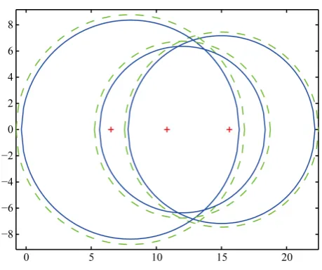
A , by Theorem 4, the eigenvalue inclusion set of Aβ is

{

} {

}

1 λ λ 15 6.8200 λ λ 8 7.6400 λ λ 12 7.7500 .

Γ = − ≤ ∪ − ≤ ∪ − ≤

From Theorem 4 of [2], the eigenvalue inclusion set of Aβ is

{

} {

}

1 λ λ 15 7.1412 λ λ 8 8.2824 λ λ 12 8.4118 .

′

Γ = − ≤ ∪ − ≤ ∪ − ≤

We use Figure 1 to illustrate Γ ⊂ Γ₁ ₁′. And the eigenvalues of A β are denoted by “+” in Figure 1. The

blue dotted line and green dashed line denote the corresponding discs Γ₁ and Γ₁′ respectively.

Meanwhile, since

β

∈N_r

( )

A ∩N_c

( )

A , by taking α=0.5 in Theorem 5, the eigenvalue inclusion set of

β

(9)

[image:9.595.200.431.83.268.2]

Figure 1. The blue dotted line and green dashed line denote the corresponding discs Γ1 and Γ1′, respectively.

Figure 2. The blue dotted line and green dashed line denote the corresponding discs Γ₂ and Γ₂′, respectively.

{

} {

}

2 λ λ 15 7.1733 λ λ 8 8.3654 λ λ 12 6.3596 .

Γ = − ≤ ∪ − ≤ ∪ − ≤

From Theorem 5 of [2], the eigenvalue inclusion set of A β is

{

} {

}

2 λ λ 15 7.4492 λ λ 8 8.7751 λ λ 12 6.7544 .

′

Γ = − ≤ ∪ − ≤ ∪ − ≤

We use Figure 2 to illustrate Γ ⊂ Γ₂ ′₂. And the eigenvalues of A β are denoted by “+” in Figure 2. The

blue dotted line and green dashed line denote the corresponding discs Γ₂ and Γ₂′ respectively. It is clear that

1 2

Γ _Γ and Γ₂Γ₁.

References

[1] Cvetković, Lj. (2009) A New Subclass of h-Matrices. Applied Mathematics and Computation, 208, 206-210. http://dx.doi.org/10.1016/j.amc.2008.11.037

[2] Liu, J.Z. and Huang, Z.J. (2010) The Dominant Degree and Disc Theorem for the Schur Complement. Applied Ma-thematics and Computation, 215, 4055-4066. http://dx.doi.org/10.1016/j.amc.2009.12.063

[image:9.595.199.429.303.495.2]

(10)

http://dx.doi.org/10.1017/CBO9780511840371

[4] Carlson, D. and Markham, T. (1979) Schur Complements on Diagonally Dominant Matrices. Czechoslovak Mathe-matical Journal, 29, 246-251.

[5] Ikramov, K.D. (1989) Invariance of the Brauer Diagonal Dominance in Gaussian Elimination. Moscow University Computational Mathematics and Cybernetics, 2, 91-94.

[6] Li, B. and Tsatsomeros, M. (1997) Doubly Diagonally Dominant Matrices. Linear Algebra and Its Applications, 261, 221-235. http://dx.doi.org/10.1016/S0024-3795(96)00406-5

[7] Smith, R. (1992) Some Interlacing Properties of the Schur Complement of a Hermitian Matrix. Linear Algebra and Its Applications, 177, 137-144. http://dx.doi.org/10.1016/0024-3795(92)90321-Z

[8] Zhang, F.Z. (2005) The Schur Complement and Its Applications. Springer-Verlag, New York. http://dx.doi.org/10.1007/b105056

[9] Demmel, J.W. (1997) Applied Numerical Linear Algebra. SIAM, Philadephia.

[10] Golub, G.H. and Van Loan, C.F. (1996) Matrix Computations. 3rd Edition, Johns Hopkins University Press, Baltimore. [11] Kress, R. (1998) Numerical Analysis. Springer, New York. http://dx.doi.org/10.1007/978-1-4612-0599-9

[12] Xiang, S.H. and Zhang, S.L. (2006) A Convergence Analysis of Block Accelerated Over-Relaxation Iterative Methods for Weak Block H-Matrices to Partition π. Linear Algebra and Its Applications, 418, 20-32.

http://dx.doi.org/10.1016/j.laa.2006.01.013

[13] Liu, J.Z., Li, J.C., Huang, Z.H. and Kong, X. (2008) Some Properties on Schur Complement and Diagonal Schur Com-plement of Some Diagonally Dominant Matrices. Linear Algebra and Its Applications, 428, 1009-1030.

[14] Liu, J.Z. and Huang, Y.Q. (2004) The Schur Complements of Generalized Doubly Diagonally Dominant Matrices. Li-near Algebra and Its Applications, 378, 231-244. http://dx.doi.org/10.1016/j.laa.2003.09.012

[15] Liu, J.Z. and Huang, Y.Q. (2004) Some Properties on Schur Complements of H-Matrices and Diagonally Dominant Matrices. Linear Algebra and Its Applications, 389, 365-380. http://dx.doi.org/10.1016/j.laa.2004.04.012

[16] Liu, J.Z. and Huang, Z.J. (2010) The Schur Complements of γ-Diagonally and Product γ-Diagonally Dominant Matrix and their Disc Separation. Linear Algebra and Its Applications, 432, 1090-1104.

[17] Liu, J.Z. and Zhang, F.Z. (2005) Disc Separation of the Schur Complements of Diagonally Dominant Matrices and Determinantal Bounds. SIAM Journal on Matrix Analysis and Applications, 27, 665-674.

http://dx.doi.org/10.1137/040620369