Spatial Distance Preservation based Methods for
Non-Linear Dimensionality Reduction
Rashmi Gupta
Member IEEE,Department of Electronics and Communication
Engineering, Ambedkar Institute of Advanced Communication Technologies and Research, Affiliated to Guru Gobind Singh
Indraprastha University, Delhi, India.
Pooja Pandey
Department of Electronics and Communication Engineering,
Ambedkar Institute of Advanced Communication Technologies and Research, Affiliated to Guru Gobind Singh
Indraprastha University, Delhi, India.
Rajiv Kapoor
Member IEEE,Departmentof Electronics and Communication
Engineering,
Delhi Technological University (Formerly Delhi College of
Engineering), Delhi, India.
ABSTRACT
The preservation of the pairwise distances measured in a data set ensures that the low dimensional embedding inherits the main geometric properties of the data like the local neighborhood relationships. In this paper, distance preserving technique namely, Sammons nonlinear mapping (Sammon‟s NLM) and Curvilinear Component Analysis (CCA) have been discussed and compared for non-linear dimensionality reduction. Basic principle in both the technique is that local neighborhood relationship is maintained. The results have beencompared for both the techniques on artificially generated data set using MATLAB software.
General Terms
Neighborhood relationship, Variance, PCA, Manifold, Non-linear, Convergence.
Keywords
MDS, Dimensionality Reduction, Nonlinear Mapping, Vector Quantization, Quasi Newton Optimization, Gradient Descent.
1.
INTRODUCTION
Basic meaning of dimensionality reduction is the transformation of a high dimensional data to a meaningful representation of low dimensional data [1]. There are various techniques which are used for dimensionality reduction like distance preserving technique and topology preserving technique. In this paper main emphasis is on „Distance Preserving Technique‟. Historically distance preservation has been the first criterion used to achieve dimensionality reduction in a nonlinear way [5]. In the linear case, simple criterion like maximizing the variance preservation or minimizing the reconstruction error, combined with a basic linear model, lead to robust method like Principal Component Analysis (PCA) and Multi-Dimensional Scaling (MDS) [2-3]. In the nonlinear case however the use of same simple criteria requires the definition of more complex data models, which is little bit difficult. In this context distance preservation appears as a nongenerative way to perform dimensionality reduction [12]. The criterion does not need any explicit model: no assumption is made about the mapping from latent variables to the observed ones. The motivation behind distance preservation is that any manifold can be fully described by pairwise distance [3-4]. Hence if low-dimensional representation can be built in such a way that the initial distances are reproduced, then the dimensionality reduction is successful [9]: the information content conveyed by the manifold its geometrical structure is preserved. It is clear that
if close points are kept close and if far points remain far, then the initial manifold and its low dimensional embedding share the same shape [10-13]. This is the basic approach which is used in all two techniques discussed in this paper. First technique which is discussed is Sammon‟s nonlinear mapping, which is a nonlinear technique. Main objective of this technique is to preserve the structure of data through Nonlinear mapping from high dimension to low dimension [4]. Second technique which is discussed is CCA [6-7]. Thistechnique mainly uses the concept of vector quantization [7-8]. It is a first method to combine the concept of vector quantization along with dimensionality reduction [11]. In this work emphasis is mainly given to show how these techniques perform the embedding from high dimension to low dimension by preserving the distance between the data points.This paper is organized as follows: Section 2 describes the CCA and Sammons nonlinear mapping theoretical concepts in detail. Experimental results are shown in Section 3. Finally the conclusions are drawn in Section 4
.
2.DISTANCE PRESERVATION BASED
TECHNIQUES
2.1 Sammon’s Nonlinear Mapping
It is a method proposed by Sammon to establish a mapping between a high dimensional space and a lower dimensional one. It is a nonlinear technique. The concept of Sammon‟s NLM is closely related to MDS. But in this case no generative model is used like MDS only a stress function is defined. Consequently the low dimensional representation can be totally different from the distribution of the true latent variables. Sammons NLM minimizes the following stress function:
2
( ( , ) ( , ))
1
1, ( , )
d i j d i j
N x y
E
i i j
c dx i j
(
1)
Where
d
y
( , )
i j
is a distance measure between ith and jth points in the P-dimensional latent spacedx( , )i j is a distance measure between the ith and jth points in the D-dimensional data space (P<D) and normalizing constant C is defined as:( , )
1, x
N
c d i j
i i j
From eqn. (1) we find there is a factor
1
( , )
which is weighting the summed terms is clear: It gives less importance to errors made on large distances. More precisely the weighting factor simply adjusts the importance to be given to each distance in Sammon‟s stress, according to its value: the preservation of long distances is less important than the preservation of shorter ones, and therefore the weighting factor is chosen to be inversely proportional to the distance. Thus our main motive is to minimize this Stress function. The optimization technique which is used to minimize above function is Quasi-Newton optimization which is iterative in nature. This optimization method is a good tradeoff between the exact Newton method, which involves the Hessian matrix, and a gradient descent, which is less efficient. From the concept of Quasi-Newton update rule, the parameter yk (i) can
be updated as follows:
( ) ( ) ( ) 2 2 ( ) E
yk i
y i y i
k k
E
yk i
(2)Where α is called as magic factor and Sammon recommends its value between 0.3 and 0.4.
Minimization of Stress Function can be achieved in following ways:
( , )
( )
( , )
( )
( , )
( , )
( , )
2
1,
( , )
( )
( , )
( , ) (
( )
( ))
2
1,
( , )
( , )
d
i j
E
E
y
y
k
i
d
y
i j
y
k
i
d
i j
d
i j
d
i j
N
x
y
y
j
j i
c
d
x
i j
y
k
i
d
i j
d
i j
y
i
y
j
N
x
y
k
k
j
j i
c
d
x
i j
d
y
i j
( , )
( , )
2
(
( )
( ))
1,
( , )
( , )
d
i j
d
i j
N
x
y
y
i
y
j
k
k
j
j i
c
d
x
i j d
y
i j
(3)After this we calculate second derivative in following way: 2
2 ( , ) ( , ) ( ( ) ( ))
2
( )
2 1, ( , ) ( , ) 3
( ) ( , )
d i j d i j y i y j
N
E x y k k
j j i
c d i j d i j
y i y x dy i j
k
(4)
For getting the minima calculation of 1st derivative and 2nd derivative is required.AlgorithmSammons Nonlinear Mapping
Step1. Compute all pair wise distances
d i j
x( , )
in the D-dimensional data space.main drawback it lacks the ability to generalize the mapping to new points.
2.2 Curvilinear Component Analysis (CCA)
CCA belongs to the class of distance preserving method. CCA was actually the first method to combine Vector Quantization [9-10] with a non-linear dimensionality reduction achieved by distance preservation. Like dimensionality reduction, Vector Quantization can be defined a way to reduce the size of a data set. However, instead of lowering the dimensionality of the observation, vector quantization reduces the number of observation. In practice it is achieved by replacing the original data points with a smaller set of points called units, centroids. Vector Quantization is basically an optional preprocessing of the data. It can be applied to reduce the number of vectors in large databases, for DR method. For small databases or sparsely sampled manifolds, however, it is often better to skip Vector Quantization in order to fully exploit the available information. In other words Vector Quantization can be thought of as an “Approximator”. Inorder to reduce the data points we take round-off value or mean value between the various data points. Concept of vector quantization is shown in fig10
2
4
6
8
X
X
X
X
1
3
5
7
Fig 1: 1-D vector quantization
All the points between 0-2 are considered as one point at 1.Similarly for other points values are taken.
Stress or Error Function which is minimizes by CCA can be defined as: 1 2 (( ( , ) ( , )) ( ( , )) 1, 1 2 N
E dx i j dy i j F dy i j
i j
(
5)
Where,
d
y
( , )
i j
is the Euclidean distances in the embedding space of dimension P (P<D) and dx( , )i j is the Euclidean distance in the data space of dimension D.To maintain the global shape of the manifold it is always require preserving the short distance as compare to longer distance. That‟s why
F
is typically chosen as a monotonically decreasing function of its argument. But inCCA we find that
F
depends on the distances in the embedding space which are varying and could temporarily be very small. While in sammon‟s stress function, the weighting depends on the constant distance measured in the data space. The optimization procedure which is used to determine the minimization of equation (5) can be calculated as:d
E E y
( )
( )
( )
y i
y i
E
y i
(7)Where α is a positive learning rate scheduled according to the Robbins-Monro condition.
The embedding of highly folded manifolds requires focusing on short distances .Longer distances have to be stretched in order to achieve the unfolding and their contribution must be lowered in stress function „E‟. Therefore
F
is usually chosen as a positive and decreasing function.For example(
)
exp(
d y
)
F
d y
(
8)
Where
controls the decreaseAlgorithm
(CCA)
Step1. Perform the vector Quantization to reduce the size of data set, if required.
Step2. Compute all pair wise Euclidean distances
d i j
x( , )
in the D-dimensional data space.Step3. Initialize the P-dimensional coordinates of all points y(i),either randomly or on the hyper plane spanned by the first principal components. Let q be equal to 1.
Step4. Give the learning rate α and the neighborhood width
their scheduled value for epoch no. Q.Step5. Select a point Y (i), and update all other ones according to update rule.(Using equation 6 and 7)
Step6. Return to step 5 until all points y (i) have been selected exactly once during the current epoch.
Step7. Increase Q and if convergence is not achieved return to step 4.
By comparison with Sammon‟s NLM, CCA proves much more flexible, mainly because the user can choose and
parameterize the weighting function
F
in equation (5) atwill. This allows one to limit the range of considered distances and focus on the preservation of distances on a
given scale only. Moreover the weighting function
F
depends on the distances measured in the embedding space this allows tearing some regions of the manifold .This is better solution than crushing the manifold, like Sammon‟s NLM does.
3.
RESULT
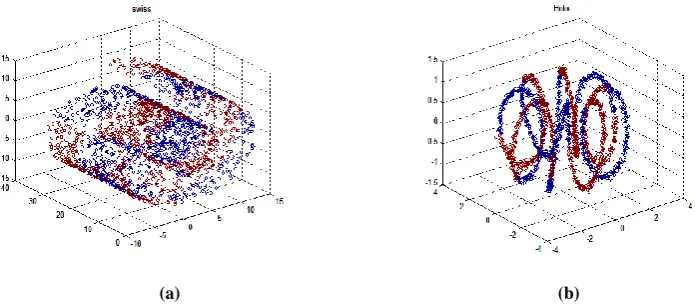
[image:3.595.116.464.431.585.2]In this section results of the proposed algorithm are presented for some artificially generated data set: Swissroll and Helix. All artificial Data set consists of 2,000 samples. Fig. 2shows the data set on which different techniques are applied These data set is in 3-D. Fig 3 shows the result of two techniques CCA and Sammons Nonlinear Mapping on Swiss roll data set. Fig 4 shows the result of both the techniques applied on Helix Data set. 3-D data set are converted to 2-D. After analysis of result (as shown in Fig.3 and 4), it is found that data points are not bijective in case of Sammon‟s nonlinear mapping. Superposition of data points occurs from one curve to the other. In other words we can say that Euclidean distance between the data points in the embedded space is not maintained, which is the important criteria for getting the error free result
(a) (b)
Fig 3: Results of Dimensionality Reduction on Swiss Roll Data Set
Fig4: Results of Dimensionality Reduction on Helix Data Set
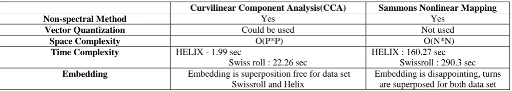
In case of Helix data set also the result of Sammon‟s Nonlinear Mapping is disappointing. But the result of CCA is much more convincing. In this case we find that the result is almost superposition free (from Fig.2 and3). Euclidean distance between the data points is maintained in a much closer sense in the Embedding space too. This is what we achieve from visualization point of view. Other criteria of comparison between the two techniques are Time Complexity and Space Complexity. In CCA Space Complexity is much less as compare to Sammon‟s Nonlinear mapping because the number of data points get reduced after vector quantization. In this data points get reduced from „N‟ to „P‟ (N<P) Unlike
Sammon‟s Nonlinear mapping in which data points are „N‟. Along with this Time Complexity for both the data set is also less in case of CCA as compare to Sammon‟s Nonlinear Mapping. Time complexity is calculated during the run time of both algorithms. All this comparison between the two techniques can be summarized in Table1. Both the techniques are Non-spectral method. Non-spectral method gives better tradeoff between computation time and flexibility than spectral methods (which is used in the technique like PCA, MDS). In this method we choose an objective function and accordingly we choose an adequate optimization technique. But in spectral method we mainly use the concept of EVD.
Table 1
.
Curvilinear Component Analysis(CCA) Sammons Nonlinear Mapping
Non-spectral Method Yes Yes
Vector Quantization Could be used Not used
Space Complexity O(P*P) O(N*N)
Time Complexity HELIX - 1.99 sec
Swiss roll : 22.26 sec
HELIX : 160.27 sec Swissroll : 290.3 sec Embedding Embedding is superposition free for data set
Swissroll and Helix
[image:4.595.49.549.535.624.2][3] H. Robins and S.Monro. 22:400-407, 1951 A stochastic approximation methods. Annals of Mathematical Statistics.
[4] E.Pekalska, D. de Ridder, R.P.W. Duin, and M.A. Kraaijveld,1999 A new method of generalizing Sammon mapping with application to algorithm speed-up. In M. Boasson, J.A. Kaandorp, J.F.M. Tonino, and M.G. Vosselman, editors, Proceedings of ASCI‟99, 5th Annual Conference of Advanced School for Computing and Imaging, pages 221-228. ASCI, Delft, the Netherlands, June
[5] J.W. Sammon.1969 A nonlinear mapping algorithm for data structure analysis. IEEE Transactions on Computers, CC-18(5):401-409.
[6] P. Dermatines and J. Herault, September 1995 CCA: Curvilinear component analysis. In 15th Workshop GRETSI, Juan-les-Pins (France).
[7] P. Dermatines and J. Herault. January 1984 Curvilinear component analysis. A self-organizing neutral network for nonlinear mapping of data sets. IEEE Transactions on Neutral Networks, 8(1):148-154.
[8] P. Dermatines and J. Herault, 1993. Vector quantization and projection neural network. Volume 686 of Lecture Notes in Computer Science, pages 328-333. Springer-Verlag, New York,
[9] Gray, R.M, Stanford university, Stanford, CA, U.S.A, April 1984. Vector Quantization, Volume:1 Issue:2 ASSP Magazine, IEEE, Volume:1 Issue:2.
[10] Rashmi Gupta and Rajiv Kapoor, August-2012, Extension and Analysis of Local Nonlinear Techniques, vol. 51-No.13.
[11] Lu Xu, Yang Xu, Tommy W.S. Chow, Pattern Recognition (43),2010, Department of Electronic Engineering, City University of Hong Kong, 83 Tat Chee Avenue, Kowloon, Hong Kong,Elsevier Ltd.
[12] Jigang Sun, Malcolm Crowe, Colin Fyfe, 2013. Incorporating visualization quality measures to curvilinear component analysis, 2012, Information Science 223, 75-101.