Software Reliability Growth Models with Log-logistic
Testing-Effort Function: A Comparative Study
N. Ahmad and Md. Zafar Imam
University Department of Statistics and Computer Applications T. M. Bhagalpur University, Bhagalpur-812007, India
ABSTRACT
Software reliability growth model is one of the basic techniques to assess software reliability quantitatively and it provides the essential information for software development activities. In this paper we compare the predictive capability of popular software reliability growth models (SRGM), such as exponential growth, delayed S-shaped growth and inflection S-shaped growth models. We first review the log-logistic testing-effort function and also discuss exponential type and S-shaped types SRGM with log-logistic testing-effort. We analyze the real data applications and compare the predictive capability of these SRGM. The experimental results reveal that inflection S-shaped type SRGM has better prediction capability as compare to exponential type SRGM.
Keywords
Software reliability growth models, testing-effort function, software testing, non-homogeneous Poisson process, estimation methods.
1.
INTRODUCTION
Software reliability is defined as the probability of failure-free operation of a computer program for a specified time in a specified environment (Musa et al., 1987; Lyu, 1996) and is a key factor in software development process. Numerous software reliability growth models (SRGMs) have been developed during the last three decades and they have applied successfully in practice to improve software reliability (Musa et al., 1987; Xie, 1991; Lyu, 1996; Pham, 2000).
In the past years, several SRGMs based on NHPP which incorporates the testing–effort functions (TEF) have been proposed by many authors (Yamada et al., 1984; 1986; 1993; Yamada and Ohtera, 1990; Huang et al., 2007; Kuoet al., 2001; Ahmad et al. 2008; 2010; Bokhari and Ahmad, 2006; Quadriet al., 2011). Currently, Ahmad et al. (2010a; 2011) also proposed a new SRGM with Log-logistic testing-effort functions to predict the behavior of failure and fault of software.
This paper first reviews the Log-logistic testing-effort function and then incorporates the Log-logistic testing-effort function into exponential and S-shaped NHPP growth models. Actual data applications are analyzed and the predictive capability of these two SRGM is compared.
2.
REVIEW OF LOG-LOGISTIC
TESTING-EFFORT
Recently, Bokhari and Ahmad, 2006 and Ahmad et al. (2010a; 2011) proposed Log-logistic testing-effort function to predict the behavior of failure and fault of a software product. They have shown that Log-logistic testing-effort function is very suitable and more flexible testing resource for assessing the reliability of software products. The cumulative testing-effort expenditure consumed in (0, t] is depicted in the following:
1
( ) [1 {1 ( ) } ]
W t t [( t) / (1 ( t) )], t0. (1)
Therefore, the current testing-effort expenditure at testing t is given by:
1 2
( ) [ ( ) ] / [1 ( ) ]
w t t t ,t0,0,0,0.(2)
where
is the total amount of testing-effort consumption required by software testing, is the scale parameter, and
is the shape parameter.The testing-effort
w t
( )
reaches its maximum value at time1
max
1 1
1
t
3.
SOFTWARE RELIABILITY
GROWTH MODELS WITH TESTING
EFFORT
In this section, we have discussed three basic software reliability growth models, such as Exponential growth model, delayed S-shaped, and inflection S-shaped growth models. These models have been shown to be very useful in fitting software failure data.
3.1
Exponential Type SRGM with
Log-logistic testing-effort
1985; Yamada et al., 1986; 1993; Yamada and Ohtera, 1990; Bokhari and Ahmad, 2006):
( )
/ ( ) ( ) , 0, 0 1
dm t
w t b a m t a b
dt , (3)
where
m
(
t
)
represent the expected mean number of errors detected in time(
0
,
t
]
which is assumed to be a bounded non-decreasing function oft
withm
(
0
)
0
,w
(
t
)
is the current testing-effort expenditure at timet
,a
is the expected number of initial error in the system, and b is the error detection rate per unit testing-effort at timet
. Solving the above differential equation, we have( )
( ) (1 bW t)
m t a e (4) Substituting W t( )from (1), we get
( )
( )
1 ( )
( ) (1 )
t b
t
m t a e
. (5)
This is an NHPP model with mean value function considering the Log-logistic testing-effort expenditure.
3.2
Delayed S-shaped Type SRGM with
Log-logistic testing-effort
Delayed S-shaped NHPP model was proposed by Yamada et al. (1984). Later, Huang et al. (2007) modified this model and incorporated the logistic testing-effort in an NHPP growth model. On the basis of assumptions (Huang et al., 2007), we obtain the following differential equation:
( ) 1
( ) ( )
( ) dm t
t a m t
dt w t , (6)
where 2 ( ) , 1 r t t rt
r( 0) is the inflection rate and
represents the proportion of independent errors present in the software. Solving (6) with the initial condition that, at
0, ( ) 0, ( ) 0
t W t m t , we obtain the mean value function
( )
1 ( )
( )
(1
)
rW ta W t
m t
r
e . (7)Substituting W t( )from (1), we get
( ) /(1 ( ) )
1 ( ) / (1 ( ) )
( )
a(1
t t)
r t tm t
r
e
. (8)3.3
Inflection S-shaped Type SRGM with
Log-logistic testing-effort
Ohba (1984; 1984a) raised the inflection S-shaped NHPP model. Later, Ahmad et al. (2011) modified the inflection S-shaped model and incorporated the Log-logistic testing-effort in an NHPP growth model.
On the basis of assumptions, if the error detection rate with respect to current testing-effort expenditures is proportional to the number of detectable errors in the software and the proportionality increases linearly with each additional error removal, we obtain the following differential equation:
( ) 1
( ) ( )
( ) dm t
t a m t
dt w t , (9) where
( ) ( )t b r (1 r)m t ,
a
( 0)
r
is the inflection rate and represents the proportion of independent errors present in the software. Solving (9) with the initial condition that, at t0,W t( ) 0, m t( )0, we obtain the mean value function:( ) ( )
1
1 ((1 ) / )
( )
bW t bW t a r re
m t
e
. (10)Substituting
W
(
t
)
from (1), we get[( ) /(1 ( ) )] [( ) /(1 ( ) )] 1
1 ((1 ) / )
( )
b t t
b t t
a r r e m t e
. (11)4.
ESTIMATION OF PARAMETERS BY
LEAST SQUARE METHOD
Least Square Estimation (LSE) technique is used to estimate the model parameters (Musa et al., 1987; Musa, 1999; Lyu, 1996). It minimizes the sum of squares of the deviations between what we expect and what we actually observe. That is, we can estimate the parameters
,
, and
of the logistic testing function in (1) and the parametersa
,b
, andr
given in (5), (8), and (11) by the method of least squares. These estimates can be obtained by minimizing the following:2 1 ( , , ) ( ) n k k k
S W W t
2 1 ( , , ) = ( ) n k k kS a b r m m t
interval
(
0
,
t
k]
and m t( )k is the estimated cumulative number of detected errors in (5), (8), and (11).Table I: Summary of studied actual data sets.
Data Set References Errors Removed Observation Period Software Project
DS1 Ohba (1984) 328, after 3.5 years: 188 19 weeks PL/1 application software, Execution Time: 47.65CPU hours, Size: 1317000 line of code
DS2 Musa et al. (1987) 136, after a long time of testing: 358 21 weeks Rome Air Development Center Project, Execution Time: 25.3 CPU hours, Size: 21700 line of code
5.
COMPARISON OF PREDICTIVE
CAPABILITY
Least Square estimation (LSE) techniques are used to estimate the model parameters (Musa et al., 1987; Musa, 1999; Lyu, 1996; Ahmad et al., 2008; 2010; 2011). The parameters of the SRGM are estimated based upon the data given in Table I. In order to compare predictive capability of exponential growth model and inflection S-shaped model with LLTEF, experiments on two actual software failure data are performed. The description of the data sets is given in Table I.
5.1 Predictive Validity
The predictive validity is defined (Musa et al., 1987; Musa, 1999) as the capability of the model to predict future failure behavior from present and past failure behavior. Assume that we have observed
q
failures by the end of test timet
q. Weuse the failure data up to time
t
e(
t
q)
to determine the parameters ofm t
( )
. Substituting the estimates of these parameters in the mean value function yields the estimate of the number of failuresm t
ˆ ( )
q byt
q. The estimate is compared with the actually observed numberq
. This procedure is repeated for various values oft
e. The ratioˆ ( )q
m t q
q
is called the relative predictive error (RPE). Values close to zero for RPE indicate more accurate prediction and hence a better model. We can visually check the predictive validity by plotting the relative error for normalized test time
t
e/
t
q.DS 1: Table II lists the comparisons of exponential growth model and inflection S-shaped growth model with LLTEF. Results reveal that the inflection S-shaped growth model with LLTEF has better performance. We compute the relative error in prediction of exponential growth model and inflection S-
shaped growth model with LLTEF for this data set. Results are presented in Tables III and IV. Figures 1 and 2 show the relative error plotted against the percentage of data used (that is,
t
e/
t
q). Figures 1, 2 and Tables II, III, IV reveal that the [image:3.595.320.536.413.615.2]inflection S-shaped growth model with LLTEF predicts the future behavior well as compare to exponential growth model.
Table II: Comparison results of exponential model and inflection S-shaped model
Model a r b AE
(%)
MSE
Exponential model with LLTEF
565.73 0.0196 58.02 116.74
Inflection S-shaped model with LLTEF
385.63 0.37 0.0622 7.54 87.69
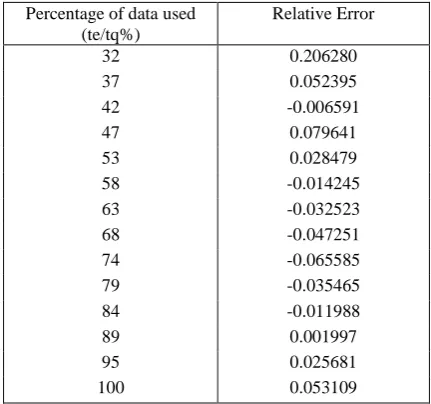
Table III: Relative error of exponential growth model
Percentage of data used (te/tq%)
Relative Error
32 0.206280
37 0.052395
42 -0.006591
47 0.079641
53 0.028479
58 -0.014245
63 -0.032523
68 -0.047251
74 -0.065585
79 -0.035465
84 -0.011988
89 0.001997
95 0.025681
100 0.053109
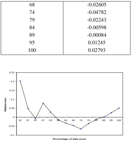
Table IV: Relative error of inflection S-shaped model
Percentage of data used (te/tq%)
Relative Error
32 0.15391
37 0.02753
42 -0.01371
47 0.08569
53 0.04369
58 0.00592
[image:3.595.321.537.654.767.2]68 -0.02605
74 -0.04782
79 -0.02243
84 -0.00598
89 -0.00084
95 0.01245
[image:4.595.57.278.70.307.2]100 0.02793
[image:4.595.314.541.72.126.2]Figure 1: Predictive Relative Error Curve of exponential growth model with LLTEF
Figure 2: Predictive Relative Error Curve of inflection S-shaped growth model with LLTEF
[image:4.595.315.540.165.563.2]DS 2: Table V shows the comparisons of exponential model and inflection S-shaped model with LLTEF. Results in the table reveal that the inflection S-shaped model has better performance for this data set. The relative error in prediction is calculated for exponential growth model and inflection S-shaped growth model with LLTEF and the results are presented in Tables VI and VII. These results are shown graphically in Figures 3 and 4. Finally, from the Figures and Tables, it can be concluded that the inflection S-shaped model gets reasonable prediction as compare to exponential model.
Table V. Comparison results of exponential model and inflection S-shaped model
Model a r b AE
(%)
MSE
Exponential model with LLTEF
133.28 0.1571 29.11 100.18
Inflection S-shaped model with LLTEF
161.02 168.37 0.0011 14.36 75.19
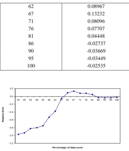
Table VI. Relative error of exponential growth model
Percentage of data used (te/tq%)
Relative Error
24 -0.979329
29 -0.949302
33 -0.869559
38 -0.852834
43 -0.814512
48 -0.642782
52 -0.507276
57 -0.201915
62 -0.019577
67 0.083816
71 0.081938
76 0.102183
81 0.072370
86 -0.008853
90 -0.029318
95 -0.037738
100 -0.037529
Figure 3: Predictive Relative Error Curve of exponential model
Table VII. Relative error of inflection S-shaped model
Percentage of data used (te/tq%)
Relative Error
24 -0.97151
29 -0.93019
33 -0.82091
38 -0.79932
43 -0.75063
48 -0.53194
52 -0.38056
57 -0.05245
-0.1 -0.05 0 0.05 0.1 0.15 0.2 0.25
32 37 42 47 53 58 63 68 74 79 84 89 95 100
Pe rce ntage of data us e d
R
el
at
iv
e
er
ro
r
-0.1 -0.05 0 0.05 0.1 0.15 0.2
32 37 42 47 53 58 63 68 74 79 84 89 95 100
Pe rce ntage of data us e d
re
la
tiv
e
er
ro
r
-1.2 -1 -0.8 -0.6 -0.4 -0.2 0 0.2
24 29 33 38 43 48 52 57 62 67 71 76 81 86 90 95 100
Percentage of data used
R
e
la
ti
v
e
e
rr
o
[image:4.595.314.543.176.437.2] [image:4.595.59.289.365.501.2] [image:4.595.52.284.694.771.2]62 0.08967
67 0.13232
71 0.08096
76 0.07707
81 0.04448
86 -0.02737
90 -0.03669
95 -0.03449
[image:5.595.55.276.67.326.2]100 -0.02535
Figure 4: Predictive Relative Error Curve of inflection S-shaped model
6.
CONCLUSION
This paper discussed exponential type and S-shaped type SRGMs with Log-logistic testing-effort. We estimated the parameters and analyzed the predictive capability of exponential growth and S-shaped growth models with LLTEF for the actual data applications. We then compared its predictive capability. The findings reveal that inflection S-shaped type SRGM has better prediction capability as compare to exponential type SRGM.
7.
ACKNOWLEDGMENTS
The authors are thankful to the Editor and the Reviewers for their valuable comments and suggestions to improve the manuscript.
8.
REFERENCES
[1] Ahmad, N., Bokhari, M. U., Quadri, S. M. K. and Khan, M. G. M. (2008), “The Exponetiated Weibull Software Reliability Growth Model with Various Testing-Efforts and Optimal Release Policy: A Performance Analysis”, International Journal of Quality and Reliability Management, Vol. 25 (2), 211– 235.
[2] Ahmad, N., Khan, M. G. M. and Islam, S. F. (2012), “Optimal Allocation of Testing Resource for Modular Software based on Testing-Effort Dependent Software Reliability Growth”, in Proceedings of the third International Conference on Computing Communication & Networking Technologies (ICCCNT-2012), IEEE Computer Society, Coimbatore, India, pp. 1-7.
[3] Ahmad, N., Khan, M.G.M and Rafi, L.S. (2011), “Analysis of an Inflection S-shaped Software Reliability Model Considering Log-logistic Testing-Effort and Imperfect Debugging”, International Journal of Computer Science and Network Security, Vol. 11 (1), pp. 161 – 171.
[4] Ahmad, N., Khan, M.G.M and Rafi, L.S. (2010), “A Study of Testing-Effort Dependent Inflection S-Shaped Software Reliability Growth Models with Imperfect Debugging”, International Journal of Quality and Reliability Management, Vol. 27 (1), pp. 89 – 110. [5] Ahmad, N., Khan, M.G.M and Rafi, L.S. (2010a),
“Software Reliability Modeling Incorporating Log-Logistic Testing-Effort with Imperfect Debugging”, in Proceedings of the International Conference on Modeling, Optimization and Computing (ICMOC-2010), Durgapur, India, Published by American Institute of Physics, pp. 651 – 657
[6] Ahmad, N., Quadri, S.M.K. and Razeef, M. (2011), “Comparison of Predictive Capability of Software Reliability Growth Models with Exponentiated Weibull Distribution”, International Journal of Computer Applications, DOI 10.5120/1949-2607, Vol. 15 (6), pp. 40–43.
[7] Bokhari, M.U. and Ahmad, N. (2006), “Analysis of a Software Reliability Growth Models: the Case of Log-logistic Test-effort Function”, in: Proceedings of the 17th IASTED International Conference on Modeling and Simulation (MS’2006), Montreal, Canada, pp. 540-545. [8] Goel, A.L. and Okumoto, K. (1979), “Time Dependent
Error-detection Rate Model for Software Reliability and Other Performance Measures”, IEEE Transactions on Reliability, Vol. R- 28, No. 3, pp. 206-211.
[9] Huang, C.Y., Kuo, S.Y. and Lyu, M.R. (2007), “An Assessment of Testing-effort Dependent Software Reliability Growth Models”, IEEE Transactions on Reliability, Vol. 56, no.2, pp. 198-211.
[10]Kuo, S.Y., Hung, C.Y. and Lyu, M.R. (2001), “Framework for Modeling Software Reliability, Using Various Testing-efforts and Fault Detection Rates”, IEEE Transactions on Reliability, Vol. 50, no.3, pp 310-320.
[11]Lyu, M.R. (1996), Handbook of Software Reliability Engineering, McGraw- Hill.
[12]Musa J.D. (1999), Software Reliability Engineering: More Reliable Software, Faster Development and Testing, McGraw-Hill.
[13]Musa, J.D., Iannino, A. and Okumoto, K. (1987), Software Reliability: Measurement, Prediction and Application, McGraw-Hill.
[14]Ohba, M. (1984), “Software Reliability Analysis Models” IBM Journal. Research Development, Vol. 28, no. 4, pp. 428-443.
[15]Ohba, M. (1984a), “Inflection S-shaped Software Reliability Growth Models”, Stochastic Models in Reliability Theory (Osaki, S. and Hatoyama, Y. Editors), pp. 144-162, Springer-Verlag, Merlin.
[16]Pham, H. (2000), Software Reliability, Springer-Verlag, New York.
[17]Quadri, S.M.K., Ahmad, N., and Farooq, S.U. (2011), “Software Reliability Growth Modeling with Generalized Exponential Testing-effort and Optimal Software Release Policy”, Global Journal of Computer Science and Technology, Vol. 11 (2), pp. 26 – 41.
-1.2 -1.0 -0.8 -0.6 -0.4 -0.2 0.0 0.2
24 29 33 38 43 48 52 57 62 67 71 76 81 86 90 95 100
Percentage of data used
R
e
la
ti
v
e
E
rr
o
[18]Xie, M. (1991), Software Reliability Modeling, World Scientific Publication, Singapore.
[19]Yamada, S., Hishitani J. and Osaki, S. (1993), “Software reliability growth model with Weibull testing-effort: a model and application”, IEEE Transactions on Reliability, Vol. R-42, pp. 100-105.
[20]Yamada, S., Ohba, M. and Osaki, S. (1984), “S-shaped Software Reliability Growth Models and their Applications”, IEEE Transactions on Reliability, Vol. R-33, pp. 289-292.
[21]Yamada, S. and Ohtera, H. (1990), “Software Reliability Growth Models for Testing Effort Control”, European Journal of Operational Research, Vol. 46, 3, pp. 343-349. [22]Yamada, S., Ohtera, H. and Norihisa, H. (1986), “Software Reliability Growth Model with Testing-effort”, IEEE Transactions on Reliability, Vol. R-35, no. 1, pp.19-23.