Tibia Bone Segmentation in X ray Images A Comparative Analysis

Tibia Bone Segmentation in X-ray Images - A

Comparative Analysis

Nathanael .E. Jacob

VIT, Pune.Country- India

M.V. Wyawahare

ABSTRACT

Segmentation techniques in the medical field are used to segment anatomical structures or other region of interest from medical images obtained from different modalities. This paper deals with segmentation techniques like manual thresholding, Otsu thresholding, watershed, traditional active contours and growcut in X-ray modality, for segmenting the tibia bone. This paper analyzes the performance of these algorithms on a database of 48 clinical X-ray images. The images have been obtained from different X-ray machines and vary in their resolution and dimensions. The performance of the algorithms have been measured and validated empirically.

General Terms

Medical imaging, machine vision, biomedical image analysis.

Keywords

X-ray, tibia bone, segmentation, growcut, validation.

1.

INTRODUCTION

A common ailment that affects the tibia bone is fractures and account for approximately 20% occupancy in hospitals [1]. The fractures that occur in tibia bones are varied and pose difficulties to a doctor in finding and assessing them accurately. Misdiagnosis of fractures can occur in clinical setting due to factors such as a tired radiologist, huge volume of data to be analyzed; satisfaction of search etc [2].This can result in loss of money, time and litigations. Therefore there is a need to design systems that can aid experts in assessing bone anomalies.

Development in machine vision can enable doctors to use computers as second opinion to diagnose fractures in bone. [3]. Such systems called Computer aided diagnosis (CAD) systems can prove very useful to analyze large volumes of medical data, as well as improve the accuracy of interpretation while reducing time for diagnosis. A CAD for fracture detection system consists of four blocks: preprocessing, segmentation, fracture detection and location of fracture [4]. This is shown in the Fig 1 below.

Fig 1: Block diagram of bone fracture CAD system

This paper deals with the first and second blocks. It focuses on applying threshold based, region based, deformable model and cellular automata based segmentation techniques to solve the problem of segmenting tibia bone accurately from X-ray images. This is followed by validation of segmentation using

time, sensitivity, specificity, Jaccard and Dice coefficients as performance metrics.

2.

RELATED WORK

Segmentation of bones plays an important role not only in fracture detection [5] but also surgery, quantitative analysis and planning for surgery. Segmentation has been researched in different modalities like CT, MRI and ray. In case of X-ray images the segmentation is quite challenging. This is because of bone boundaries being less clear in X-ray images as compared to images in CT or MRI [6].

Region based algorithm involving region growing, region merging and region labelling has been applied by [7] Manos et al. to segment hand and wrist bones. [8] El-Feghi et al. used a fuzzy set algorithm to segment bone in lateral skull x-ray images. The algorithm however suffers from the problem of disjoined segmented regions. [9] Vinhais et al. segmented the rib cage in posterior-anterior chest X-ray images using a deformable prior model, which is deformed using a deformation grid. The segmented output defines the lung region, which is used in Computer aided diagnosis system. On the other hand [10] Zhanjun Yue et al., rib finding algorithm uses Hough transform to approximate and finally localize the rib bones using active contour model in chest radiographs. Geodesic active contour incorporating prior shape information has been used by [11] Yuchong Jiang et al. to segment the leg bone. The algorithm is robust to background noise of the casting material overlaying on the fractured leg. [12] Ying Chen et al. worked on developing a model based code to automatically extract femur bone from X-ray images. Initially a model femur contour is registered to the x-ray image, followed by active contour with shape constrains to refine the contour. [13] G. Behielset al. uses active shape model (ASM), involving a regularizing smoothness constrain to segment femur, humer and calcaneus bones in the human body.

3.

PREPROCESSING

Algorithm:

1. Start

2. Read input image, I

3. Resize the input image I, by a scale of 0.15 to get the resized image Iresized.

4. Apply Otsu segmentation [14] to the image, Iresized.

5. Calculate area of every region in the threshold image, Iotsu.

6. Select the region with maximum area as the ROI. 7. Calculate its inclination.

8. Correct the inclination of the bone using the formula 8.1. If the bone is inclined to the right, then it is rotated

in anti-clockwise direction by an angle equal to “90-angle” (i.e. Anglecorrected= 90 - Angleoriginal)

8.2. But if the bone is inclined to the left, then it is rotated in clockwise direction by an angle equal to “-90-angle” (i.e. Anglecorrected = - 90 -

Angleoriginal). Here the value obtained will be

negative. This denotes that the image should be rotated in clockwise direction.

9. The new image obtained is Irot. Next, the co-ordinates of

the bounding box of the maximum area region in the above image are obtained.

10. Using these coordinates a rectangle containing the bone region (ROI) is cropped from the image Irot. The new

image obtained is Icrop, which is the final pre-processed

image I_new. 11. Stop

The size of test images obtained after pre-processing fall in the following range: height = 367 – 530 (in pixels) and width = 50 – 191 (in pixels).One of the results is shown in Table 1.

Table 1. Preprocessing result

Before After

Image

Size (in pixels) 2446 x 2010 461 x 100

Angles (in degree) 60.22543 0

The segmentation algorithms adopted must be robust to such interpolated images, obtained due to pre-processing. Once the ROI is obtained from segmentation, the binary mask of the ROI is rescaled and rotated back to its original size and inclination. The binary mask is then used to crop the ROI from the original, unaltered medical image. This ensures that the final ROI obtained contains pixels having intensities that have been originally provided to the segmentation system and the system is in no way modifying the intensities of the ROI by processing it.

Prior to segmentation, the images are rotated and scaled. Scaling and rotation of images involve interpolation. The less frequently this technique is used, the lesser is the distortion in the image. This is because interpolation never adds additional details to an image other than what is already present. Interpolation adopts the strategy of guessing pixel values at additional new locations based on the neighbouring pixel values of those locations. This causes loss of quality of images and hence is generally avoided on sensitive medical images

4.

SEGMENTATION METHODS

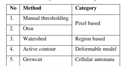
The methods discussed in this section are categorized in Table 2.

Table 2. Segmentation Techniques No Method Category

1. Manual thresholding

Pixel based 2. Otsu

3. Watershed Region based 4. Active contour Deformable model 5. Growcut Cellular automata The following section explains the concepts behind the segmentation techniques.

4.1

MANUAL THRESHOLDING

Manual thresholding requires user effort for selecting the right threshold value and is usually done with the help of a histogram, using trial and error method. It involves converting the input image into binary image based on a fixed threshold. The input image pixels having intensities greater than the threshold level are assigned the value 1 and all the other pixels are assigned the value 0 in the output image. The manual thresholding does not hold good since the intensity distribution range for the 3 classes (Skin, bone and background) is not unique and varies with different images as well as the X-ray modality used. Often the three classes are found to overlap for a given area on the histogram. Due to these reasons this method is not suitable for tibia bone segmentation problem. The segmentation result for a threshold value of 153 is shown in Table 3.

4.2

OTSU THRESHOLDING

Table 3. Manual thresholding results

Input Image Segmented Tibia bone

X

-ra

y

M

ac

h

in

e

1

X

-ra

y

M

ac

h

in

e

2

Here three thresholds are found using Otsu method. The first threshold (T1) is only good enough to segment the leg from the background. So in order to get the bone the leg region is provided to the Otsu algorithm to get the second threshold (T2). But this results in over segmentation. So the region having intensities between T1 and T2 is provided to the algorithm to get a third threshold (T3). This has been tested to give better results than T1 and T2.

The Threshold values can be shown on the intensity axis as follows:-

Fig 2: Threshold values on the intensity axis

The threshold values are: T1 = 108, T2 = 191 and T3 = 151 for the example shown in Table 4.

Table 4. Otsu segmentation results

Input Image

Segmented Tibia bone

for T1

Segmented Tibia bone

for T2

Segmented Tibia bone

for T3

4.3

WATERSHED SEGMENTATION [15]

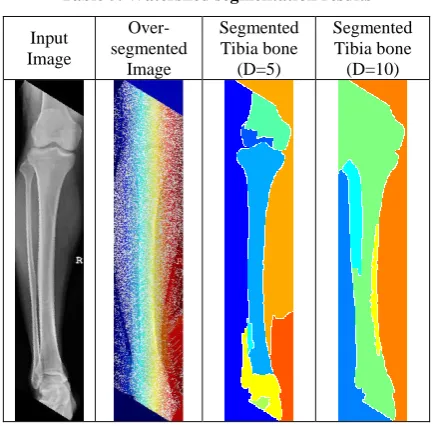
The watershed segmentation is known to face over segmentation error due to irregularities in the gradient of the image to be segmented. To overcome this markers are defined on the image from where, the topological surface is flooded. The algorithm used in Matlab for watershed segmentation is the Meyer‟s flooding algorithm developed in the early 1990‟s. A disc marker of radius 5 or 10 has been used to obtain the results. The size of marker to be used for a given image is empirically set. The results obtained using the above approach is shown below.

Different regions of the Watershed output for one of the input images have been indicated by different colours in Table 5.

Table 5. Watershed segmentation results

Input Image

Over- segmented

Image

Segmented Tibia bone

(D=5)

Segmented Tibia bone (D=10)

4.4

ACTIVE CONTOUR

SEGMENTATION

Active contours [16] or Snakes are widely used for edge detection in the field of image processing. A snake can be defined as a spline curve which tends to minimize its energy. The energy of the snake is dependent on its shape (internal energy) and its location (external energy). The total energy of the snake is given by:-

The above equation involves a parametric snake given by s(p) = (x(p),y(p)). Eint and Eext are the internal and external energies of the snake.

Eint can is given by the formula,

It controls the mechanical behaviour of the snake by determining its shape. Here α and β are constants. If alpha is less, the snake can elongate more and if beta is less the snake can bend more. The internal energy is meant to force the snake to be small and smooth.

Eext is given by the equation,

It depends on the properties of the image. The simplest form of external energy is the inverse of the gradient magnitude of the input image.

Internal and external forces determine the shape and position of the snake. The internal force keeps the snake smooth whereas the external force guides the snake towards the image features.

The output of the snake model is a closed contour. This is very advantages if the region boundary has discontinuities. The snake tends to take the general shape of the image boundary. Also the edges of output of the snake model are very fine. This will prove to be advantages if ones interest lies in extracting features pertaining to the edges.

Table 6. Active contour segmentation results

Input Image

External Force Field

Spline Image

Segmented Tibia bone

However the active contour method is known to face problems at concavities. Furthermore the snake needs to be initialized close to the ROI. This is often done manually. The snake is found to be highly sensitive to its parameters which are initialized empirically to values that vary for different types of images. The result for AC model is given in Table 6.

4.5

GROWCUT

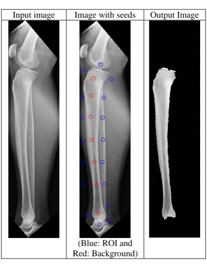
GrowCut [17] segmentation is an interactive process, modelled by evolution of cellular automata. Here every pixel in an image can be considered as a cell. The cells can be initialized as foreground, background, or undefined. As the algorithm proceeds, these cells compete to dominate the image domain. Some cells capture their neighbours, replacing their labels. The ability of a cell to spread depends on its feature vector and strength. There can be more than 2 class labels in an image. It can be extended to N dimensions. The growcut involves „for‟ loops which prove to be computationally expensive in Matlab. To solve this problem, the code for growcut has been written in C in Matlab (i.e. as a binary mex file). Mex stands for Matlab executable.

The most important challenged faced in applying the growcut algorithm is the computation time for large medical images. The results reported in the original paper of growcut [17], mention a segmentation time of 4 sec for a 256x256 image on a 2.5 GHz processor. However for large images the computation time required is 10 minutes, which is quite large. To address this problem the images were resized. The mex code for growcut has been implemented by Shawn Lankton and can be downloaded from [18].

The results obtained are given in Table 7.

Table 7. Active contour segmentation results

Input image Image with seeds Output Image

(Blue: ROI and Red: Background)

5.

VALIDATION

develop more better and efficient codes, evaluation parameters will be needed [20] .These parameters help to evaluate the quality or “goodness” of image segmented by the above algorithms. In general validation techniques can be categorized as follows:-

1. Analytical 2. Empirical

a. Empirical Goodness b. Empirical Discrepancy

The paper uses empirical discrepancy method for validation and analysis.

Since the output of a segmentation algorithm is affected by multiple parameters, it is not possible that a single evaluation parameter will prove effective in evaluating the “goodness” of segmentation. Therefore four metrics have been used to validate the segmentation results. They include: Sensitivity, Specificity, Jaccard and Dice co-efficient. The parameters are chosen, such that they complement each other in their ability to evaluate a segmented output. The ground truth images have been produced manually, by tracing a polygon on the boundaries of the tibia bone in the X-ray images.

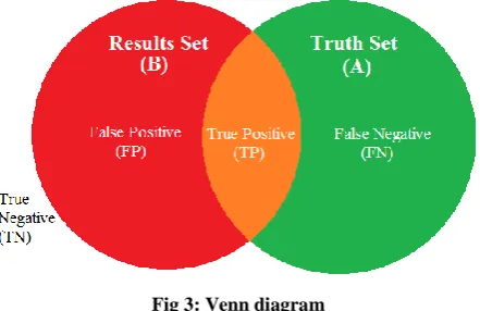
The Venn diagram below will help to visualize the spatial differences between a Segmented output (Results set) and its corresponding gold standard (Truth set) [21]

Fig 3: Venn diagram

Let X be the set of all pixels in the image. Then set A is the set of pixels identified as tibia bone by gold standard segmentation and B is the set of pixels identified as tibia bone by a segmentation algorithm. True positive set (TP) is then defined as the set of pixels identified as tibia bone by both gold standard and user defined segmentation.

i.e. TP = A ∩ B

True Negative set (TN) is the set of pixels identified as non-tibia bone by both the algorithms.

TN = (A ∪ B)’

Similarly False Positive (FP) and False Negative (FN) are given as,

FP = (A‟ ∩ B) and FN = (A ∩ B‟)

Using these regions four evaluation parameters are defined as, 1. Sensitivity = TP/(TP + FN)

2. Specificity = TN/(TN + FP)

3. Jaccard Co-efficient = TP/(FP + TP + FN) 4. Dice Co-efficient = 2TP/(FP + 2TP + FN)

1. Sensitivity (S)

It measures the proportion of tibia bone pixels that have been accurately segmented by the segmentation algorithm. Using sensitivity, false negative rate (fnr) is obtained and is given by:-

False negative rate (%) = (1-sensitivity) x 100 Since sensitivity gives the amount of foreground pixels correctly segmented as foreground pixels, false negativity rate can be defined at the percentage of foreground pixels classified as background pixels or in other words false negative rate is the percentage of under segmentation error.

2. Specificity (Sp)

Similarly using specificity, false positive rate (fpr) is defined as the percentage of over segmentation error and is given by:-

False positive rate (%) = (1-specificity) x 100

3. Similarity metrics a) Jaccard co-efficient (J)

The Jaccard co-efficient measures the ratio of area of overlap between the segmented output and the ground truth to the union of their areas. This is defined as:-

J = |A ∩ B| / |A ∪ B|

b) Dice co-efficient (D)

The dice co-efficient is another metric used to define segmentation quality or measure of similarity between the segmented image and the gold standard image. It is defined as:-

J = 2 |A ∩ B| / (|A| ∪ |B|)

The dice co-efficient is more commonly used parameter to measure spatial overlap and is used when the number of non-ROI pixels is greater than the number of non-ROI pixels [22]. Using the Jaccard co-efficient, the dice co-efficient can be easily obtained, since the dice efficient and Jaccard co-efficient are equivalent to each other and there exists a monotonic relationship between them i.e.

D=2J / (1+J)

Both the coefficients give value between 0 and 1. Here 1 implies perfect similarity of the segmented image to its gold standard and 0 implies total dissimilarity between the two. The Jaccard co-efficient gives a low percentage of similarity as compared to Dice co-efficient for cases where the spatial overlap is very less [23].

However both the Jaccard and dice coefficients are unable to distinguish between over and under segmentation errors and assume equal cost for both these errors. Also small errors in the segmented image cannot be identified by these parameters [22].

Table 8. Averages of validation parameters

Methods

AVERAGES t (sec) fnr

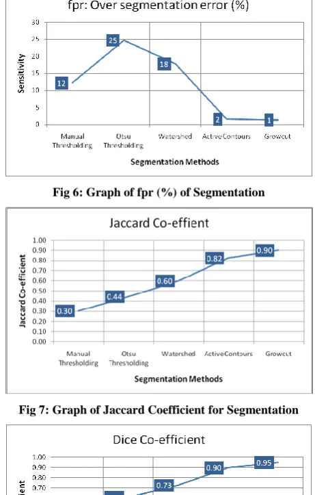
(%) fpr (%)

J D

Manual Thresholding 0.40 54 12 0.30 0.44 Otsu Thresholding 0.48 17 25 0.44 0.61 Watershed 0.89 17 18 0.60 0.73 Active Contours 8.69 13 2 0.82 0.90 Growcut 3.78 6 1 0.90 0.95

For the sake of analysis, the average values of every parameter are plotted against the segmentation methods in Figs 4 to 8.

Fig 4: Graph of Segmentation time

The first three segmentation algorithms give results in very less time as compare to Active contour and Growcut. However their accuracy is less. Active contour and Growcut however give better segmentation results with an increase in computation time. Among active contour and growcut, growcut is less computationally expensive with higher accuracy and is worth considering for automation.

Fig 5: Graph of fnr (%) of Segmentation

Sensitivity gives an idea of accuracy as well as segmentation error. Manual segmentation gives a very low value which implies poor segmentation. This is because of an under segmentation (fnr) error of 54% and over segmentation (fpr) error of 12%. Otsu, watershed, active contour and growcut give a reasonably good value in the range 0.8 – 0.9. However Otsu gives a low value of specificity in the range 0.75 ± 0.07 and records a maximum over segmentation error (fpr) of 25%. Watershed gives the same value of 0.8 for sensitivity and specificity, which implies a reasonably good segmentation. Active contour has recorded a higher value for both sensitivity

and specificity as compared to watershed which means that its accuracy is higher compared to watershed. Its relatively higher value for specificity as compared to sensitivity implies that it suffers more from under segmentation error as compared to over segmentation error. Growcut performs the best among the 5 techniques and records a low value of 6% and 1% of under and over segmentation error respectively.

Fig 6: Graph of fpr (%) of Segmentation

Fig 7: Graph of Jaccard Coefficient for Segmentation

Fig 8: Graph of Dice Co-efficient for Segmentation

The average error information for the segmentation methods are provided by the Jaccard and Dice similarity metrics. Their ideal value is one for perfect segmentation and less than one if either one of the under or over segmentation errors occur. They record a high value only if both the segmentation errors are low.

6.

CONCLUSIONS

Based on the analysis the following points can be concluded:- 1. Intensity based algorithms fail to successfully

segment bone from X-ray images because of the intensity distribution of the bone and skin classes. There is no perfect separation of classes occurring in the histogram of the X-ray images. This cases over or under segmentation, which cannot be corrected even by normal morphological operations like region filling, image close, image open etc. 2. Although the watershed segmentation gives results

in very less time, the accuracy offered by the technique is unsuitable for medical applications. Also the selection of marker size has to be automated.

3. Active contour in its most basic form seems to give accurate result, but the process of selecting the snake parameters to give such results is tedious and is empirical in nature. Also it suffers from the problem of detecting concave boundaries at the end of the tibia bone. Therefore a better implementation of active contours is needed that can solve the issues. One such method is the GVF implementation of active contours.

4. Growcut has been proved to give better results as compared to Otsu, watershed and active contours both in terms of accuracy and speed of segmentation. Although the method appears promising, automation of growcut segmentation is essential if the technique is to have practical significance in the medical field. Automating the seed selection step will prove to be challenging. Also the automation process will tend to reduce the accuracy of the algorithm.

7.

FUTURE SCOPE

The importance of bone segmentation can be understood in clinical analysis, where it can be used for computer aided diagnosis and surgery [24]. Future work can include designing a computer aided diagnosis system (CAD). It is unlikely that such systems can replace surgeons because CAD is a system where both physicians and computers play complementary roles. Such systems will definitely help in assisting doctors in reducing diagnosis time and increasing accuracy of diagnosis. In future CAD and PACS (Picture archiving and communication systems) may be combined and used as a single unit for clinical diagnosis [25].

Future work can include designing a bone fracture computer aided diagnosis system (CAD). In such systems after successfully segmenting the bone image from X-ray, the next step for a fracture detection system would be to extract features from the segmented region. Once the features of interest unique to a normal and fractured bone have been obtained, various classifiers can then be used to classify the segmented bone as normal or fractured. A fractured bone can be further classified based on the type of fracture. Some of the classifiers that can be implemented are Bayesian, Neural networks, SVM etc.

8.

ACKNOWLEDGMENTS

The authors would like to thank Dr. Kapil Kapadnis (Poona Hospital), Dr. Hemant Deshmukh (KEM Hospital, Mumbai) and Dr. Ashwini Kulkarni (Deenanath Mangeshkar Hospital,

Pune) for their support in providing us the X-ray image database. Also a special thanks to the technicians Mr.Sanatan, Mr.Vinay and Miss Usha.

9.

REFERENCES

[1] Chipchase, L. S., K. McCaul, and T. C. Hearn. "Hip fracture rates in South Australia: Into the next century." Australian and New Zealand Journal of Surgery 70.2 (2000): 117-119.

[2] Berbaum, Kevin S., and Edmund A. Franken. "Satisfaction of Search in Radiographic Modalities." Radiology 261.3 (2011): 1000-1001. [3] Giger, Maryellen L. "Computer-aided diagnosis in

medical imaging-a new era in image interpretation." Medical Imaging Ultrasound (2000): 75-79.

[4] Umadevi, N., and S. N. Geethalakshmi. "Enhanced Segmentation Method for bone structure and diaphysis extraction from x-ray images." International Journal of Computer Applications 37.3 (2012): 30-36.

[5] Nathanael E Jacob and M V Wyawahare. “Survey of Bone Fracture Detection Techniques.” International Journal of Computer Applications 71.17(2013):31-34. [6] Ding, Feng, Wee Kheng Leow, and Tet Sen Howe.

"Automatic segmentation of femur bones in anterior-posterior pelvis x-ray images." Computer Analysis of Images and Patterns. Springer Berlin Heidelberg, 2007. [7] Manos, G. K., et al. "Segmenting radiographs of the hand

and wrist." Computer Methods and Programs in Biomedicine 43.3 (1994): 227-237.

[8] El-Feghi, I., et al. "X-ray image segmentation using auto adaptive fuzzy index measure." Circuits and Systems, 2004. MWSCAS'04. The 2004 47th Midwest Symposium on. Vol. 3. IEEE, 2004.

[9] Vinhais, Carlos, and Aurélio Campilho. "Genetic model-based segmentation of chest x-ray images using free form deformations." Image Analysis and Recognition. Springer Berlin Heidelberg, 2005. 958-965.

[10] Yue, Zhanjun, Ardeshir Goshtasby, and Laurens V. Ackerman. "Automatic detection of rib borders in chest radiographs." Medical Imaging, IEEE Transactions on 14.3 (1995): 525-536.

[11] Jiang, Yuchong, and Paul Babyn. "X-ray bone fracture segmentation by incorporating global shape model priors into geodesic active contours."International Congress Series. Vol. 1268. Elsevier, 2004.

[12] Chen, Ying, et al. "Automatic extraction of femur contours from hip x-ray images." Computer Vision for Biomedical Image Applications. Springer Berlin Heidelberg, 2005. 200-209.

[13] Behiels, Gert, et al. "Active shape model-based segmentation of digital X-ray images." Medical Image Computing and Computer-Assisted Intervention– MICCAI‟99. Springer Berlin Heidelberg, 1999.

[14] Otsu, Nobuyuki. "A threshold selection method from gray-level histograms."Automatica 11.285-296 (1975): 23-27.

[16] Kass, Michael, Andrew Witkin, and Demetri Terzopoulos. "Snakes: Active contour models." International journal of computer vision 1.4 (1988): 321-331.

[17] Vezhnevets, Vladimir, and Vadim Konouchine. "GrowCut: Interactive multi-label ND image segmentation by cellular automata." proc. of Graphicon. 2005.

[18] http://www.shawnlankton.com/?s=growcut.

[19] Torsney-Weir, Thomas, et al. "Tuner: Principled parameter finding for image segmentation algorithms using visual response surface exploration."Visualization and Computer Graphics, IEEE Transactions on 17.12 (2011): 1892-1901.

[20] Zhang, Yu Jin. "A survey on evaluation methods for image segmentation."Pattern recognition 29.8 (1996): 1335-1346.

[21] 52. Shattuck, David W., et al. "Online resource for validation of brain segmentation methods." NeuroImage 45.2 (2009): 431-439.

[22] Tahmasebi, Amir M., et al. "A validation framework for probabilistic maps using Heschl's gyrus as a model." Neuroimage 50.2 (2010): 532-544.

[23] Manning, Christopher D., and Hinrich Schütze. Foundations of statistical natural language processing. Vol. 999. Cambridge: MIT press, 1999. [24] Pham, Dzung L., Chenyang Xu, and Jerry L. Prince.

"Current methods in medical image segmentation 1." Annual review of biomedical engineering 2.1 (2000): 315-337.

[25] Doi, Kunio. "Computer-aided diagnosis in medical imaging: historical review, current status and future potential." Computerized medical imaging and graphics: the official journal of the Computerized Medical Imaging