Particle Swarm Optimization (PSO) based Tool Position Error Optimization

(1)

Particle Swarm Optimization (PSO) based Tool Position

Error Optimization

Prasant Kumar

Mahapatra

Biomedical Instrumentation Division (V-2), CSIR-Central

Scientific Instruments Organisation(CSIO), Sector-30,

Chandigarh 160030, India

Spardha

Scientific Instruments Organisation(CSIO), Sector-30,

Chandigarh 160030, India and UIET, PU, Chandigarh

Inderdeep Kaur

Aulakh

University Institute of Engineering and Technology

(UIET), Panjab University, Sector-25, Chandigarh 160014,

India

Amod Kumar

Scientific Instruments Organisation(CSIO),Sector-30,

Chandigarh 160030, India

Swapna Devi

National Institute of Technical Teachers’ Training and Research (NITTTR), Sector-26, Chandigarh 160026, India

ABSTRACT

High-precision tool positioning is one of the fundamental requirements for the industry now-a-days. Earlier, tool positioning and its verification were done using sensors etc. In this paper, an algorithm has been proposed to increase the tool positioning accuracy by analyzing the information obtained using CCD camera. The images of lathe tool are used for carrying out the experiments. Firstly, the images of lathe tool, before and after movement, are captured. From these images, the distance traversed by the tool is calculated which is the observed distance. Tool positioning can be achieved accurately if the errors arising out of target (distance expected to be traversed by the tool) and observed position of the tool are optimized. This paper addresses positional errors and presents an error optimization method using arithmetic measures such as mean, median and Particle Swarm Optimization (PSO) based nature-inspired technique. Finally, the results of the two arithmetic measures are compared with the results of PSO which shows the capability of PSO to converge towards the optimal solution.

General Terms

Soft Computing, Error Optimization

Keywords

Tool positioning, Error Optimization, Particle Swarm Optimization, Image Processing

1. INTRODUCTION

The push to improve the performance of various mechanical tools has led to the identification and correction of errors in the manufacturing industry. Different errors that are expected to occur may be due to

using sensors. To further improve the performance and hence the precision of the system, soft-computing techniques such as Artificial Neural Network (ANN), Fuzzy Logic, and Particle Swarm Optimization (PSO) have been employed [2-4]. Further, sensors have been replaced by CCD cameras to measure tool wear and tear [5]. But soft-computing techniques, on the data obtained using cameras, for tool position monitoring have been rarely applied till date. In this paper, the authors have proposed to apply Particle Swarm Optimization (PSO), a nature-inspired technique for minimizing the tool positional error as much as possible. The positional errors occur mainlydue to inaccurate positioning of the tool after the movement as observed through images.

PSO has been applied to a wide variety of optimization applications such as electrical distribution system [6], image clustering performance improvement [7], parameter optimization of tile manufacturing process [8], finding optimal routing path [9], higher calibration accuracy of three-axis magnetometer [10] etc. and also for optimization of Artificial Neural Networks [11]. Here, the capability of PSO is used for optimizing the positional errors of the tool.

The PSO method was implemented to improve the accuracy of the tool positioning in both horizontal and vertical axis. Initially, the arithmetic measures such as mean and median were employed to compute the positional errors. Further, the results of the two measures were compared with the results obtained using PSO which proved the efficiency of PSO over the arithmetic measures.

(2)

2. OVERVIEW OF PARTICLE

SWARM OPTIMIZATION (PSO)

PSO is a technique proposed by James Kennedy and Russell Eberhart in 1995 [12]. PSO mimics the behavior of birds for the optimization process. The birds are also known as particles which fly in the search space to find the optimal solution. Each particle in the search space occupies a particular position and moves with certain velocity representing a solution set. The particle updates its position, PD and velocity, VD according to certain optimal

solution in its neighborhood, lBest (localbest) or the optimal solution of the complete swarm, gBest (globalbest), PgD. Many parameters, controlling the acceleration of the particles, are also associated with PSO. The particles move in the search space according to the optimal position in the neighborhood. The movement of the particles leading to convergence towards the optimal solution is shown in Figure 1 [13].

The position of a particle is updated using equations in [14]

Xi+1=Xi+Vi+1 (1)

where Xi=Particle position

Vi=Particle velocity

The velocity is calculated as:

Vi+1=Vi+C1R1 (Pi-Xi) + C2R2(Pg-Xi) (2)

where Pi=Best particle position

Pg=Best global position

Ci=Social parameters

Ri=Random number between 0 and 1

3. EXPERIMENTAL SETUP

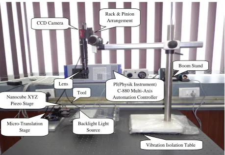
Computer-vision based system is used for carrying out experiments. The system includes hardware component and the software component. The entire hardware component is shown in Figure 2 which consists of a vibration isolation table (Thorlabs, PBG52510) for positioning the complete setup, a monochrome Charged Couple Device (CCD) camera (1.3 mega pixel, AVT Stingray) and Navitar lens (Part no.:1-60135) fitted to an adjustable mounting plate which is attached to the arm of boom stand. Advanced LED backlight (EO part no. NT66-840) is used to provide better illumination. Rack and pinion arrangement of the mounting plate is used to move the camera steadily along the X, Y directions and for interfacing the camera with PC (personal computer), a PCI express slot based IEEE 1394b card is used.

The software component includes the software code written in MATLAB for error optimization. The code is further used to analyze and process the data obtained through camera. The complete method used for coding is explained further.

pi4

Vi4

pi1

Vi1

Vi2

pi2

Vi5

pi5 piD

ViD

Vi3

pi3

pg1

Vi1

pi1

Vi3

pi3

Vi4

pi4

piD

ViD

pi5

Vi5

Vi1

Vi1 pg2

pi3

Vi3

pi5

Vi5

piD

ViD

pi1

Vi1

pi2

Vi2

pi3

(3)

[image:3.595.83.543.68.383.2]

Fig 2: Experimental setup

4. PROPOSED METHODOLOGY

Initially, the gray scale images of both start (reference image) and moved position of the tool are captured using the CCD camera. From these images, the distance traversed by the tool is calculated which is the observed distance. Then, the error is computed by differencing the observed movement from the target movement. Mathematically,

Error= Target distance- Observed distance (3) Where, target distance= distance expected to be traveled by the tool

Observed distance=distance calculated from images of start and moved position

The complete process of error calculation and optimization is described in detail later.

4.1 Obtaining Binary Images

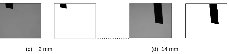
Global thresholding method [15] is used to obtain the binary images of the captured gray scale images. Thresholding basically separates foreground objects from the background preserving the image features and reducing the number of levels to only two (0 or 1). The MATLAB inbuilt functions graythresh() and im2bw() are used for this purpose. The graythresh() command selects an optimal gray level for thresholding and im2bw() generates the binary image by setting the pixels having value below the level to 0 (black) and above the level to 1 (white). The binary images thus obtained are shown in Figure 3.

Reference image (0 mm) (b) 1 mm

CCD Camera

Rack & Pinion Arrangement

Lens

Boom Stand

PI(Physik Instrument) C-880 Multi-Axis Automation Controller Tool

Nanocube XYZ Piezo Stage

Micro-Translation Stage

Backlight Light Source

(4)

………

[image:4.595.79.531.66.174.2]

(c) 2 mm (d) 14 mm

Fig 3: Gray scale and corresponding thresholded images. (a-d) Gray and thresholded images of reference, 1 mm, 2 mm and 14 mm tool movement respectively

4.2 Calculating distance travelled by the

tool

The binary images obtained above are further used to compute the distance moved by the tool. The black pixels of the binary image (Figure 3) represent the tool. The distance moved can be computed by calculating the edge to edge movement or between each black pixel of the moved and the reference image. Here, the distance between each black pixel is used. The distance is calculated in number of pixels using Euclidean distance, ED [16] formula as:

ED= (𝑥2 − 𝑥1)2

_{+ (𝑦2 − 𝑦1)}

2 ₍₄₎

where x1, y1 are the pixel coordinates of reference image and x2, y2 are the pixel coordinates of moved image

4.3 Calculating the real-world distance

traversed by the tool

A process known as calibration is used for computing the real-world distance. In this process, the real-world dimension of a single pixel is computed using EO grid [17] and LED backlight illumination. The images of EO grid having dimension of 25mm by 25mm are captured using camera. The total number of pixels is found out in that grid. Then total number of pixels is equated with 25mm dimension to compute the dimensions of a single pixel. The real-world dimension of a single pixel came out to be 0.0267 mm. The real-world dimensions of a single pixel thus calculated are multiplied with the ED (in pixels) moved by each pixel of the tool to compute the real-world distance.

4.4 Applying arithmetic measures

The arithmetic measures such as mean and median are applied further on the real-world distances calculated above to get the distance moved by the tool as a whole. The applied techniques are explained as follows:

Median=middle value, if number of ED is odd, else Median=average of middle two values, if number of ED is

even and

where n is the number of ED, X= Value of ED

(5)

[image:5.595.73.545.90.717.2]

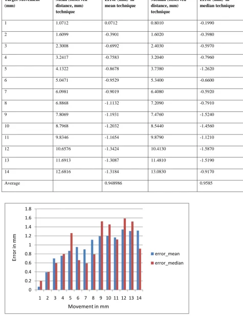
Table 1. Observed distances and the errors obtained using mean and median techniques

0 0.2 0.4 0.6 0.8 1 1.2 1.4 1.6 1.8

1 2 3 4 5 6 7 8 9 10 11 12 13 14

error_mean

error_median

Movement in mm

Erro

r

in

m

Target Movement (mm)

Mean (observed distance, mm) technique

Error (mm) in mean technique

Median (observed distance, mm) technique

Error (mm) in median technique

1 1.0712 0.0712 0.8010 -0.1990

2 1.6099 -0.3901 1.6020 -0.3980

3 2.3008 -0.6992 2.4030 -0.5970

4 3.2417 -0.7583 3.2040 -0.7960

5 4.1322 -0.8678 3.7380 -1.2620

6 5.0471 -0.9529 5.3400 -0.6600

7 6.0981 -0.9019 6.4080 -0.5920

8 6.8868 -1.1132 7.2090 -0.7910

9 7.8069 -1.1931 7.4760 -1.5240

10 8.7968 -1.2032 8.5440 -1.4560

11 9.8346 -1.1654 9.8790 -1.1210

12 10.6576 -1.3424 10.4130 -1.5870

13 11.6913 -1.3087 11.4810 -1.5190

14 12.6816 -1.3184 13.0830 -0.9170

[image:5.595.69.545.102.721.2]

(6)

4.5 Applying PSO for error optimization

The basic PSO technique is applied in the proposed algorithm. After applying PSO, the particles tend to move towards the global optimal solution. In this, each pixel covering the tool portion forms the solution set or is considered as a particle in the search space. The particles are assigned with a fitness value (the initial error), the particle’s individual best value and velocity which is the function of distance i.e., the distance moved per unit time. Each particle’s position, Ri is initialized as lying in between the maximum and minimum best value (error) of the pixels. Similarly, the velocity Vi of each particle is

initialized as varying between maximum and minimum velocity of the particles. Further, velocity of each particle is updated using equation:

V p,m ← chi*(w*(V p,m) + rand * C1 * (pBestValue p,m-R p,m) + rand * C2 *(gBestPosition p,m- R p,m)) (6)

where C1 and C2 are the cognitive and social parameters, whose values are taken as 2.05,

w is the inertial weight which controls the impact of previous velocity on the current,

rand are the random numbers distributed between [0, 1], pBestPosition is the particle’s best position and gBestPosition is the global best position which is the position with minimum error in the search space

Particle position or error is updated using equation

R i ← R i + Vi (7)

Further, the particle’s best position (pBestPosition) is computed by using the best value in the neighborhood. In the proposed algorithm, the size of neighborhood is chosen

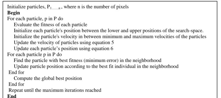
as two in all the four direction i.e., the best values of two pixels surrounding the single particle in each direction are compared. The particles update their best position with the best value (minimum error) in the neighborhood giving the lBestPosition or the local best solution of the particles within the group. The minimum error value or best value within the local best solution is used to further compute the global best solution, gBestPosition which is the optimal solution of the entire swarm. The pseudo code for the algorithm is explained below:

5. EXPERIMENTAL RESULTS

The experiments were performed using grayscale images of the lathe tool captured using the camera. The algorithm were written on MATLAB platform and the software code was tested on different movements of the tool ranging from 1-14 mm. The comparison among PSO, mean and median shows that PSO gives better results than two arithmetic measures. Table 2 demonstrates and compares the results obtained using arithmetic measures (mean and

median technique) and PSO. The negative value of error indicates that the tool is behind the target position and the positive values shows that the tool is ahead of the target position. The average error observed over 14 movements is 0.948986 for mean, 0.9585 for medianand 0.424564 for PSO. It explains the effectiveness of PSO over the other technique. Further, the results are compared graphically in Figure 5 which shows reduction in error using PSO technique.

Initialize particles, P1……n , where n is the number of pixels

Begin

For each particle, p in P do

Evaluate the fitness of each particle

Initialize each particle's position between the lower and upper positions of the search-space. Initialize the particle's velocity in between minimum and maximum velocities of the particles Update the velocity of particles using equation 5

Update each particle’s position using equation 6 For each particle p in P do

Find the particle with best fitness (minimum error) in the neighborhood Update particle position according to the best fit individual in the neighborhood End for

Compute the global best position End for

[image:6.595.75.460.323.493.2]

(7)

[image:7.595.127.548.85.731.2]

Table 2. Error obtained using mean, median and PSO techniques

Experimental Results

Target Movement (mm)

Error (mm) using Mean Technique

Error (mm) using Median Technique

Error (mm) using PSO Technique

1 0.0712 -0.1990 0.1009

2 -0.3901 -0.3980 0.3980

3 -0.6992 -0.5970 0.4090

4 -0.7583 -0.7960 0.6790

5 -0.8678 -1.2620 0.0800

6 -0.9529 -0.6600 0.6600

7 -0.9019 -0.5920 0.4290

8 -1.1132 -0.7910 0.7910

9 -1.1931 -1.5240 0.0819

10 -1.2032 -1.4560 0.3843

11 -1.1654 -1.1210 0.0497

12 -1.3424 -1.5870 0.5159

13 -1.3087 -1.5190 0.4482

14 -1.3184 -0.9170 0.9170

Average 0.948986 0.9585 0.424564

0 0.2 0.4 0.6 0.8 1 1.2 1.4 1.6 1.8

1 2 3 4 5 6 7 8 9 10 11 12 13 14

PSO

error_mean

error_median

Movement in mm

Erro

r

in

m

[image:7.595.126.549.89.507.2]

(8)

6. CONCLUSION

The proposed work is an effort to minimize the positional error of machine tools positioning used in mechanical industry and robotics etc. The authors have attempted to minimize the errors effectively by using Particle Swarm Optimization (PSO) algorithm. This resulted in precision of tool positioning in machine vision-based system both in horizontal and vertical axis. The results obtained using PSO are compared with the results obtained using arithmetic measure (mean and median) which proved the ability of PSO to carry out the optimization task more effectively. Further, many other nature inspired techniques such as artificial immune system, bacterial foraging algorithm, firefly algorithm and the latest bat algorithm may be tried for optimization and monitoring of the tool. Different techniques can also be used in combination, by selecting the best operators of each to achieve more satisfactory results.

7. ACKNOWLEDGMENTS

Authors would like to thank Director, CSIR-CSIO for his guidance during investigation.

8. REFERENCES

[1] Kennedy J. and Eberhart R. 1995.Particle swarm optimization. Proceedings of the IEEE International Conference on Neural Networks, University of Western Australia, Perth, Western Australia (27 Nov.-1 Dec.), vol. 4,1942-1948.

[2] Xiaohong R., Weidong X., Yong S. and Yinggao Y. 2011. Real-time thermal error compensation on machine tools using improved BP neural network. Proceedings of the International Conference on Electric Information and Control Engineering, Wuhan, China (April 15-17), 630-632.

[3] Zhitian W., Yuanxin W., Xiaoping H. and Meiping W. 2013. Calibration of Three-Axis Magnetometer Using Stretching Particle Swarm Optimization Algorithm. IEEE Transactions on Instrumentation and Measurement 62, 281-292.

[4] Sahoo N.C., Ganguly S. and Das D. 2012.Multi-objective planning of electrical distribution systems incorporating sectionalizing switches and tie-lines using particle swarm optimization. Swarm and Evolutionary Computation 3, 15-32.

[5] Man To W., Xiangjian H. and Wei-Chang Y. 2011. Image clustering using Particle Swarm Optimization. Proceedings of the IEEE Congress on Evolutionary Computation, New Orleans, USA (June 5-8), 262-268.

[6] Jurkovic J., Korosec M. and Kopac J. 2005.New approach in tool wear measuring technique using CCD vision system. International Journal of Machine Tools and Manufacture 45, 1023-1030.

[7] Nanda S.J. 2009 Artificial immune systems: principle, algorithms and applications. Master Thesis. Rourkela, National Institute of Technology.

[8] Yadav R. and Mandal D. 2011. Optimization of Artificial Neural Network for Speaker Recognition using Particle Swarm Optimization. International Journal of Soft Computing and Engineering 1,80-84.

[9] Gong C., Yuan J. and Ni J. 2000.Nongeometric error identification and compensation for robotic system by inverse calibration. International Journal of Machine Tools and Manufacture 40, 2119-2137.

[10]Alıcı G., Jagielski R., Ahmet Şekercioğlu Y. and Shirinzadeh B. 2006.Prediction of geometric errors of robot manipulators with Particle Swarm Optimisation method. Robotics and Autonomous Systems 54, 956-966.

[11]Schutte J. F. (2005), The Particle Swarm Optimization Algorithm [PowerPoint slides]. Retrieved fromhttps://www.google.co.in/url?sa=t&rct=j&q=&esrc =s&source=web&cd=1&ved=0CDcQFjAA&url=https% 3A%2F%2Fbitbucket.org%2F12er%2Fpso%2Fsrc%2Fe 1371b5bba75%2Fdoc%2Fliterature%2FSlides%2FPSO_ introduction.pdf&ei=tfiBUdmkAdHHrQeE14GgCA&us g=AFQjCNGcyiS37y_uhkL1bURIn3n502PvsA&sig2=C _2H0Bq3Q8dyOb2zpidAUw&bvm=bv.45960087,d.bmk

[12]Toofani A. 2012.Solving Routing Problem using Particle Swarm Optimization. International Journal of Computer Applications 52, 16-18.

[13]Huanglin Z., Yong S. and Haiyan Z. 2009.Thermal Error Compensation on Machine Tools Using Rough Set Artificial Neural Networks. Proceedings of the WRI World Congress on Computer Science and Information Engineering, Los Angeles, USA (31 Mar. - 2 April), 51-55.

[14] Navalertporn T. and Afzulpurkar N.V. 2011.Optimization of tile manufacturing process using particle swarm optimization. Swarm and Evolutionary Computation 1, 97-109.

[15]Gonzalez R.C., Woods R.E., and Eddins S.L. 2011. Digital Image Processing using MATLAB, 2nd ed., Tata McGraw-Hill Education Private Ltd, India, pp. 511-516.

[16]Shih F. Y. and Wu Y.-T. 2004. Fast Euclidean distance transformation in two scans using a 3 × 3 neighborhood. Computer Vision and Image Understanding 93, 195-205.