ABSTRACT
The real-time vehicle routing problem with time windows and simultaneous delivery products and pickup wastage materials (RT-VRPTWDPPWM) is formulated as extension of VRP. The real-time delivery/pickup demands are served by capacitated vehicles with limited initial loads. Moreover, pickup services aren’t necessarily done after delivery services in each route. A improved genetic algorithm ( master-slave genetic algorithm)is proposed. To generate offspring for the next generation for crossover (Sub Route Sequence Crossover Method (SRSCM) and for mutation (Sub Route Alter Mutation Method (SRAMM) methods are introduced. The results shows that the proposed algorithm can efficiently decrease the total route cost. Results of comparative tests are presented showing that the improved algorithm performs well on large populations.
Keywords
Genetic Algorithm (GA); Multi Objective Genetic Algorithm (MOGA); Sub Route Sequence Crossover Method (SRSCM); Sub Route Alter Mutation Method (SRAMM);Vehicle Routing Problem (VRP).
1.
INTRODUCTION
The vehicle routing problem with time windows (VRPTW) is a well-known NP-hard problem. Almost all VRPTW methods proposed are devoted to a static problem where all data are known before the route is constructed and do not change thereafter. The advancement of communication and information technology makes entrepreneurs more aware of the importance of just-in-time managerial strategies. In the past decade, express transshipment activities and e-commerce business have experienced a rapid growth. These developments have led to a gradual growth of a new class of problems, known as real-time routing and scheduling problems, where problem size and parameters change after the vehicle routes are constructed. In our research, we describe a real-time vehicle routing problem with time windows and simultaneous delivery/pickup wastage materials (real time pickup and delivery problem), an extension to traditional VRPTW [31, 32]. The problems that need to be solved in real-life situations are usually much more complicated than the classical VRP. One complication that arises in practice is that goods not only need to be brought from the depot to the customers, but also wastage product picked up at a number of customers and brought back to the depot. This problem is well
known as real-time vehicle routing problem with time windows and simultaneous delivery products and pickup wastage materials (RT-VRPTWDPPWM). RT-VRPTWDPPWM as an extension for vehicle routing problem, which is a complex combinational optimization problem, and is a well-know non-polynomial hard (NP-hard) Problem [4, 33]. RT-VRPTWDPPWM often encountered in fact, and has broad prospects in theory and practice, for example in the soft drink industry, where empty bottles must be returned, and in the delivery to grocery stores, where reusable pallets/containers are used for the transportation of merchandise [34, 35]. Reverse logistics is an important area in which the planning of vehicle routes takes the form of a RT-VRPTWDPPWM problem, as companies become interested in gaining control over the whole lifecycle of their products [36, 37]. For example, in some countries legislation forces companies to take responsibility for their products during lifetime, especially when environmental
issue are involved [38, 39]. In RT-VRPTWDPPWM some requests are made after the routes are constructed. Each of the new requests must be assigned to an appropriate vehicle in real time [40, 41]. The uncertainty comes from the occurrence of the new service requests. There is no knowledge of further incoming requests. The problem size of transport manager changes therefore in real time [42, 43]. The real-time vehicle routing problem with time windows and simultaneous delivery products and pickup wastage materials (RT-VRPTWDPPWM) can be modeled as an routing and scheduling problem.The RT-VRPTWDPPWM may involve a set of objectives usually conflicting and which have to be optimized simultaneously [44]. However optimizing one objective often happens at the expense of the others. This is the reason why a multi-objective approach may be more than relevant in this context. In this paper, the RT-VRPTWDPPWM addressed as a multi- objective combinatorial optimization problem(MCOP) with conflicting ciriteria [1, 2]. The objective function is computationally demanding. The main objective is to find a permutation of the customers (a prefixed tour) that minimizes the expected distance traveled by the vehicle and minimum number of tours, minimum routing time (means minimum servicing and travelling time). So we used non dominated solution ranking algorithm to optimize following objectives [3, 6]. Tournament selection with tournament size two is used for selection of better solutions in the population and to keep more copy of better solutions by removing worst solutions in the population. In this paper for reproduction Sub Route Sequence Crossover Method (SRSCM); Sub Route Alter Mutation Method (SRAMM) are applied. This paper is organized as follows. After introduction, a brief literature review is presented in Section 2. The RT-VRPTWDP definition and formulation described in section 3 and in section 4. In Section 5 details of multi objective optimization technique explained. In section 6 need of genetic algorithm and in 7 implementation part is narrated, where chromosome representation, proposed master-slave genetic algorithm, proposed crossover and mutation technique elaborated. To select parents for next generation tournament selection is explained. In section 8 experimental results explained.
2.
LITERATURE
REVIEW
Transportation is the most expensive logistics activity in terms of not only the transportation cost itself but also its ripple effects on the rests of processes which are sensitively affected by expected delivery time. Especially for the time constraint
Real Time Vehicle Routing Problem with Time Window
Simultaneously Delivery Products and Pick up
Wastage Materials with Proposed Master-Slave
Genetic Algorithm
Padmabati Chand J. R. Mohanty
School Of Computer Engineering School of Computer Application
KIIT University, Bhubaneswar, India KIIT University, Bhubaneswar, India
which is considered significantly for a variety of areas such as purchasing, inventory and customer delivery, on-time delivery has played an important role in improving the rest of processes and services. With growing sophisticated customer demands, the organizations and companies are under pressure to improve their transportation strategies and methods to satisfy these demands so that they can improve both service levels and fuel consumption. One of the transportation issues affecting operational performances is unexpected new demands or demand changes. In particular, if the vehicle is already operating with given delivery sequences, unexpected new demands or demand changes are very difficult to be reflected on the existing sequences. They should be applied in real-time to maintain overall transportation performance and guarantee minimum exchange costs. In terms of algorithm performance for transportation scheduling, metaheuristic or simulation methods rather than optimization approaches are usually used to reflect demand changes into existing solutions due to computational complexity. The important issue of heuristic or metaheuristic for the vehicle routing scheduling is to find appropriate methods to diversify search space and intensify routing solution to reduce both transportation cost and time gap from demands. Along with these common approaches, control theoretic approaches based on discrete event simulation have been developed recently. One of the most important benefits of this approach, in terms of algorithm performance, is quick convergence into a relatively good solution and this property provides significant benefits to highly changeable transportation environment. Reverse logistics can be defined as the reverse process of logistics. The Council of Logistics Management (CLM) defines reverse logistics as “The process of planning, implementing, and controlling the efficient, cost effective flow of raw materials, in-process inventory, finished goods and related information from the point of consumption to the point of origin for the purpose of recapturing value or proper disposal” [20, 21].The problems that need to be solved in real-life situations are usually much more complicated than the classical VRP. One complication that arises in practice is that goods not only need to be brought from the depot to the customers, but also must be picked up at a number of customers and brought back to the depot. This problem is well known as VRP with Pick-Up and Delivery (VRPPD). Vehicle routing problem with simultaneously pickup and delivery problem (VRP-SDP) as an extension for vehicle routing problem, which is a complex combinational optimization problem, and is a well-know non-polynomial hard (NP-hard) Problem. For example, in some countries legislation forces companies to take responsibility for their products during lifetime, especially when environmental issue are involved(as in the disposal of laser printers’ cartridges).Returned goods are another example where the definition of vehicle routes may take the form of a VRP-SDP problem. Owing to difficulty of the problem itself and deficiency of attention, even now little work can be found. In the literature, the VRPPD is also called VRP with Backhauls (VRPB) [18, 19]. The problem can be divided into two independent CVRPs [18, 26]; one for the delivery (linehaul) customers and one for the pickup (backhaul) customers, such that some vehicles would be designated to linehaul customers and others to backhaul customers. VRP-SDP is firstly proposed by [22], subsequently near 10 years, there are not correlative report until attach importance to reverse logistics, some researcher engaged in the problem [23, 24]. Most of the algorithms of solving the VRP-SDP are based on that of classical VRP. In recent years, most published research for the VRP-SDP has focused on the development of heuristics. Genetic algorithm (GA) is a powerful algorithm for solving engineering design and optimization problems [27, 28] and has
been used to tackle many combinatorial problems, including certain types of vehicle routing problem [25, 26]. Storn and Price [30] first introduced the differential evolutionary (DE) algorithm in 1996. DE was successfully applied to the optimization of some well-known nonlinear, non-differentiable and non-convex functions in Storn. DE combines simple arithmetic operators with the classical operators of crossover, mutation and selection to evolve from a randomly generated starting population to a final solution. DE is a population based and direct stochastic search algorithm (minimizer or maximizer), this simple, yet powerful and straightforward, features make it very attractive for numerical optimization. DE uses a rather greedy and less stochastic approach to problem solving compared to evolution algorithms. Recently, differential evolution algorithm have drawn great attention from researchers due to its robustness and flexibility and have been used to tackle many combinatorial problems, and it’s used field is fast expanding. But there are little work can be found about VRP that using differential evolution. In this paper, we developed a new extension of VRP i.e. RT-VRPTWDPPWM.
3.
PROBLEM
DEFINITION
Whenever the real time demands are generated, the routing schedule must change in response to new or altered requests. In the model we consider, there is an initial routing schedule that incorporates all works currently known. This routing schedule is adjusted as new work arrives, and can be improved providing this does not interfere with decisions that have already been committed to. To clarify the scope of the research, necessary assumptions are stated as follows:
1. There is a communication and transmission systems between the transport manager and drivers. Through the communication system, the transport manager informs the drivers which demand to serve next only when committing to that decision. Once a driver is en route to the next destination, however, he must necessarily serve this node. No diversion is allowed. 2. Real time demand means that the planning time span to transfer demand information from dispatcher to driver is short. 3. Delivery problems (delivering goods from a depot to the customer) and pickup problems (picking up wastage materials at the customer and bring back to a depot) are considered simultaneously.
4. Uncertainty comes from a single source, namely the occurrence of new requests. There is no uncertainty associated with the customer locations and travel times.
5. In a least commitment strategy, the drivers are asked to wait at their current location if some waiting time is expected at the next customer. The latest possible time allows last changes to the planned routing schedule.
6. Demand forecast is not tackled by this research. Expected quantities and occurrence times of orders can improve the solution quality of the real-time routing problem, but increase the complexity of the real-time routing problem.
7. Each customer is serviced exactly once by one vehicle. 8. Vehicle starting and ending location should be same.
4.
PROBLEM FORMULATION
In this paper following notations are used for problem definition.
n is the number of requests. C0 is the depot.
C is the set of all customers in the graph. 0 and 2n+1 are the start and end terminal respectively. K is the set of vehicles. G= (C, A) directed graph on which the problem is defined. A is the set of edges.
Q k0 is load of the vehicle k at depot 0.
Q k0i is load of the vehicle k after delivering goods from depot 0 to the demand of first customer i.
Q k i=1 j=2…N+1 &i≠j is load of the vehicle k after delivering goods from customer i to customer j.
Q k N+1 ,1,0 is load of the vehicle is wastage materials after picking from last customer to the first customer and return to the depot.
distance ij is the distance from customer i to customer j. [ei, li] time window of customer i.
di>0 duration of service at customer i. L is max deliver time of a request.
cij cost of traveling from customer i to customer j. (It is assumed that cij satisfies the triangle inequality).
tij time needed for going from customer i to customer j. (It is assumed that tij satisfies the triangle inequality).
xk
ij =1 if the kth vehicle goes straight from customer i to customer j.
L k
i is the delivery time of request i on vehicle k. P ki is the pick up time of request i on vehicle k. Subject to
Every request is served exactly once: 𝑥𝑖𝑗𝑘
𝑗 ∈𝑁
𝑘∈𝐾 = 1 i∈ 𝑁
Same vehicle starts from depot 0 and ends at the same depot:
𝑥0𝑖𝑘
𝑗 ∈𝑁 = 𝑗 ∈𝑁𝑥𝑁+10𝑘 k∈ K
The same vehicle that enters a customer leaves the customer: 𝑥𝑗𝑖𝑘
𝑗 ∈𝑁 – 𝑗 ∈𝑁𝑥𝑖𝑗𝑘 =0, k∈ 𝐾
Every vehicle enters the end terminal: 𝑥𝑖,𝑁+1𝑘
𝑖∈𝑁 = 1, k∈K
Every vehicle enters from end terminal to previous customers to first customer and return to the depot:
𝑥𝑁+1,𝑁−1,1,0𝑘
𝑖∈𝑁 = 1, k∈K
Setting and checking pick up time: (tkj+1 j + p
kj+1 )≤ cj
Setting and checking deliver time: (tkij +oj + L
k j + t
kjj+1)≤ oj+1
Setting and checking vehicle load: 𝑄𝑗𝑘≥ (𝑄𝑖𝑘+𝑞𝑗) 𝑥𝑖𝑗𝑘 i∈N, j∈ 𝑁, 𝑘 ∈ 𝐾
𝑄𝑖𝑘 ≤Q i∈N, 𝑘 ∈ 𝐾
Binary variables:
𝑥𝑖𝑗𝑘 ∈ 0,1 i∈N, j∈ 𝑁, 𝑘 ∈ 𝐾
Objective
min 𝑘∈𝐾 𝑖∈𝑁 𝑗 ∈𝑁𝑐𝑖𝑗𝑘𝑥𝑖𝑗𝑘
min 𝑘∈𝐾 𝑖∈𝑁 𝑗 ∈𝑁𝑑𝑖𝑠𝑡𝑎𝑛𝑐𝑒𝑖𝑗𝑘𝑥𝑖𝑗𝑘
min 𝑘∈𝐾 𝑖∈𝑁 𝑗 ∈𝑁𝑡𝑖𝑗𝑘𝑥𝑖𝑗𝑘
5.
M
ULTI-
OBJECTIVEG
ENETICA
LGORITHMA Multi Objective GA (MOGA) is proposed to solve multi objective problems combining both continuous and discrete variables [12, 13]. The MOGA was able to find the optimal solution for each objective function, as well as an important number of Pareto optimal solutions. Pareto optimality defines how to determine the set of optimal solutions. A solution is Pareto-optimal if no other solution can improve one objective function without a simultaneous deterioration of at least one of the other objectives. A set of such solutions is called the Pareto-optimal front [10, 11]. An example of a Pareto front is seen in Figure 1.Evolutionary algorithms (EAs) have recently attracted much attention in the exploration of Pareto-optimal fronts. It is claimed that EAs are the preeminent search algorithms for such tasks [14]. An overview of EAs in multi objective EAs can be
found in [11, 17]. Below we briefly touch on relevant terminology and definitions regarding multi objective optimization problems [15, 16]. The set of input parameters, or decision variable, is called the decision vector. The set of objective functions that measure the performance of the system is called the objective vector. In an evolutionary algorithm framework, a decision vector naturally corresponds to a candidate solution, and the functions comprising the objective vector are typically incorporated, by various techniques, into the fitness function(s) [11, 12]. A dominance test is a way to measure the relative performance among decision vectors. Given two decision vectors a and b, a dominates b if and only if a ties or exceeds b's performance on every objective, and there exists at least one objective where a's performance strictly exceeds b's. Using this test, we can pare down any given set of decision vectors and find the set of non dominated decision vectors. Such a set is said to form the non dominated front [11]. If the non dominated set resulted from testing every possible decision vector, then the non dominated set is the Pareto-optimal front. A coverage test adds a test for equality to the dominance test. Given two decision vectors a and b, a covers b if and only if a dominates b or a's objective vector is identical to b's. The dominance test will be used to cull dominated solutions produced by a given algorithm. The coverage test will be used to compare the solutions produced by algorithms head-to-head. In figure 1 pareto optimal front and in figure 2 working of genetic algorithm is explained. The outline of MOGA algorithm elaborated below. Step wise description of genetic algorithm explained in the following flow chart.
Fig.1: Pareto optimal front
Start
Step 1: Initialize population
Step 2: Repeat generation until to reach maximum generation {
Step 2(a): Decode and evaluate chromosomes of each solution in the population
Step 2(b): Count number of solutions dominated by certain individual. If j number of solutions dominated by solution i then fitness of i is j
Step 2(c): Repeat step 2(a) and 2(b) to get dominance relationship of rest of the solutions in the population
} End
varying the parameters involved in the genetic operators, GA provide an ideal platform for performing a flexible search in VRP. Genetic algorithm is widely used to solve optimization problems for its characteristic, especially vehicle routing problem [11, 12].
7.
IMPLEMENTATION
PART
7.1.
Proposed master-slave genetic algorithm
In this paper we modified the existing genetic algorithm and named as master-slave GA algorithm. Entire population is stored in master set. Population is divided into number of sub populations of equal size and store in number of slaves {slave 1, slave 2,…,slave 5}. Starting from first slave, we determined non dominated set from two slaves like from slave 1 and slave 2, kept it in another slave, suppose slave 6. Again non dominated sets from slave 2 and from slave 3 and stored it in suppose slave 7. Again non dominated set from slave 3 and slave 4 and stored it in a slave suppose slave 8. In the same way non dominated set from slave 4 and slave 5 and stored it in slave 9. Repeated the above procedure for slave 6 , 7, 8 and 9. Finally we got a single non dominated set.start
N := population size M { mi , mi+1 ,…}:= slaves n := size of the slave i :=1
for j:=1 to N for M := 1 to k if (mi ≤n)
mi [j]:=N[j] j:=j+1 end if i :=i+1 M :=M+1 end for end for
master_slave_function(M,n) {
for i:= 1 to n
find out non dominance relationship between mi and mi+1 t :=n+1
keep all the non-dominated sets in mt i:=i+1
end for
master_slave_function(M,n-1) }
end
7.2.
Chromosome Representation and Initial
Population Creation
In our approach, a chromosome has three parts. First part of the chromosome represents routes. The second part of the chromosomes indicates first node number of each sub route and the last part of the chromosome represents last node number of each sub routes. A gene in a given chromosome indicates the original node number assigned to a customer, while the sequence of genes in the chromosome indicates the order of visitation of customers. Thus, the chromosome consists of integers; where new customers are directly represented on a chromosome with their corresponding index number and each committed customer is indirectly represented within one of the groups [5, 25]. In the following figure 3, we have taken total number of route is 3 and the first node numbers of each sub route are 5, 4, 2. The last node number of each sub routes are 6, 3, 1.
7.3.
Cross Over (Sub Route Sequence
Crossover Method (SRSCM))
We utilized a problem-specific crossover operator that generatesfeasible route schedules [8, 9]. In following, we explained the proposed crossover technique. We considered two chromosomes and in each chromosome there are 9 customers. Number of sub routes in chromosome 1 is 3 and in chromosome 2 is 4.
Chromosome 1: 3 9 1- 2 5 7-8 6 4 Chromosome 2: 1 5 2-9 3 8-4-6 7
Randomly a sub route is selected from chromosome 1. Depending upon number of nodes in selected sub route, was the number of sub routes of offspring 2. Placed node number in sequence in each sub routes of offspring 2 by satisfying all the constraints. Similarly randomly a sub route is selected from Start
Read problem instance data
Set GA parameters
Generate initial
population
Decode chromosomes
Evaluate fitness function for each chromsomes
Select mates
Apply GA operators
Convergence check
End
5 7 1 4 8 3 2 9 6 5 4 2 6 3 1 First node number of each route
Last node number of each sub routes starting from last sub route
chromosome 2. Depending upon number of nodes in selected sub route, was the number of sub routes of offspring 1. Placed node number in sequence in each sub routes of offspring 1. Suppose randomly a sub route is selected from chromosome 1 i.e. 2 5 7. In selected sub route 3 nodes are there so in offspring 2 there was 3 sub routes.
Offspring 1: 9 - 3 - 8 Offspring 2: 2 - 5 -7
The visited node number which is in offspring 1 from chromosome 2 is deleted. Similarly the visited node number which was in offspring 2 from chromosome 1 is deleted. After deletion rest of the nodes in sub routes are:
Chromosome 1: 3 9 1 -8 6 4 Chromosome 2: 1 5 2-4 6 7
Randomly a sub route is selected from chromosome 1. Placed node number in sequence in each sub routes of offspring 2 after the visited node numbers by satisfying all the constraints. Similarly randomly a sub route is selected from chromosome 2. Placed node number in sequence in each sub routes of offspring 2 after the visited node numbers by satisfying all the constraints. Suppose randomly a sub route is selected from chromosome 1 i.e. 3 9 1. Placed 3 after visited node number 2 in offspring 2, similarly 9 after visited node number 5 and 1 after node number 7. While placing nodes if constraints are satisfied place in next sub routes. Other wise make new sub routes.
Offspring 1: 9 4 - 3 6 – 8 7 Offspring 2: 2 3 - 5 9 -71
The visited node number which is in offspring 1 from chromosome 2 is deleted. Similarly the visited node number which is in offspring 2 from chromosome 1 is deleted. After deletion rest of the nodes in sub routes were:
Chromosome 1: 8 6 4 Chromosome 2: 1 5 2
Sequentially rest of the node number in offspring 1 from chromosome 2 is inserted. If constraints are not satisfied then make new sub routes. Same method followed for offspring 2. So the final routes are:
Offspring 1: 9 4 1 - 3 6 – 8 72- 5 Offspring 2: 2 3 8 - 5 9 6 -71 4
7.4.
Mutation (Sub Route Alter Mutation
Method (SRAMM))
In the following steps we explained details of proposed mutation method.
Step 1: we considered a chromosome where (3 1), (2 7) and (8 4) are first and last node numbers of each sub routes.
3 9 1- 2 5 7-8 6 4
Step 2: Randomly any two pairs are selected, suppose (3 1) and (2 7). Exchanged 3 with 7 and 1 with 2 by considering all the constraints.
3 9 2- 1 5 3-8 6 4
Step 3: After exchanging, the new chromosome is: 7 9 2- 1 5 3-8 6 4
7.5.
Tournament Selection
At every generation stage, we need to select parents for mating and reproduction. Tournament selection is used to perform fitness-based selection of individuals for further evolutionary reproduction [5, 7]. In the tournament selection, tournaments are played between two solutions and the better solutions is chosen and placed in the mating pool. Two other solutions are picked again and another slot in the mating pool is filled with the better solution. If carried out systematically, each solution can be made to participate in exactly two tournaments. The best solution in a population will win both times, thereby making two copies of it in the new population. Using similar argument, the worst solution will lose in both tournaments and will be eliminated from the population. In this way any solution in a population will have zero, one or two copies in the new population. It has been shown by Goldberg and Deb that the tournament selection has better or equivalent convergence and computational time complexity properties when compared to any other reproduction operator. Tournament selection operator is that just by changing the comparison operator, the minimization and maximization problems can be handled easily and RT-VRPTWDPPWM is a minimize optimization problem.
8.
EXPERIMENTAL RESULTS
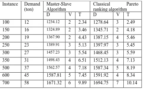
All the programs are implemented in mat lab. The program was run on an Intel Pentium IV 1.6 MHz PC with 512 MB memory. In this paper we discussed different types of evolutionary algorithm. We proposed master-slave genetic algorithm. We implemented all the algorithms by solving RT-VRPTWDPPWM. In table 1 we narrated input genetic parameters. In table 2 experimental results explained by taking different population size. Also in table 2 we compared our proposed algorithms results with classical pareto ranking algorithm. Column 3, 4, 5 narrated distance (d), number of vehicles (v) and total time (t) required to visit all the customers by applying master-slave GA. Column 6, 7 and 8 explained distance, vehicle and time required by applying classical pareto ranking algorithm. Details of classical pareto ranking algorithm we can refer [7]. In table 3 we compared our proposed SRSCM, SRAMM with one point crossover and reverse mutation methods by applying master-slave GA. Details of classical genetic operators we can refer [7]. In figure 4, 5 and 6 we explained computational results comparison of master-slave and pareto ranking algorithm for the objectives distance, vehicle and time. The comparative study of table 2 and table 3 concluded that proposed work gave better results as compared to classical algorithms.
Table 1. Genetic Parameters
Parameter Type Value
Number of runs 100
Selection Type Tournament with size 2
Generation span 1000
Crossover rate 0.8-1
Mutation rate 0.05-0.2
Crossover type SRSCM
Table 2. Result Comparison of Proposed Master-slave GA with Classical Pareto GA Algorithm
Table 3. Result Comparison of Proposed Master-slave GA with proposed genetic operators and classical crossover, mutation operators.
9.
CONCLUSION
We introduced a new extension of VRP, real-time vehicle routing problem with time windows and simultaneous delivery products and pickup wastage materials (RT-VRPTWDPPWM). In this paper we proposed an algorithm master-slave genetic algorithm. To generate offspring for next generation, new crossover and mutation methods are introduced i.e. for crossover (Sub Route Sequence Crossover Method (SRSCM) and for mutation (Sub Route Alter Mutation Method (SRAMM). By comparative study analysis we conclude that proposed methods gives better result as compared to classical algorithm.
1 2 3 4 5 6 7 8 9
0 200 400 600 800 1000 1200 1400 1600 1800
instance---->
d
is
ta
n
c
e
Master-slave pareto ranking
1 2 3 4 5 6 7 8 9
0 1 2 3 4 5 6 7
instance---->
v
e
h
ic
le
Master-slave pareto ranking
1 2 3 4 5 6 7 8 9
0 2 4 6 8 10 12
instance---->
ti
m
e
Master-slave pareto ranking
Instance Demand (ton)
Master-Slave Algorithm
Classical Pareto
ranking algorithm
D V T D V T
100 12 1234.12 2 2.34 1278.64 3 2.49
150 16 1324.89 2 3.46 1345.71 2 4.18
200 19 1367.90 2 4.43 1387.15 4 5.46
250 23 1389.91 3 5.13 1397.97 3 5.45
300 27 1457.23 3 5.54 1468.45 3 5.59
350 31 1498.43 4 6.51 1512.13 4 7.13
500 37 1562.57 4 7.18 1587.34 5 8.19
600 45 1587.81 5 7.45 1591.92 4 8.34
700 58 1671.32 6 9.89 1694.75 7 10.14
Instance Demand (ton)
Master-Slave Algorithm with SRSCM and SRAMM
Master-Slave Algorithm with One point cross over and reverse mutation
D V T D V T
100 12 1234.12 2 2.34 1245.64 2 2.40
150 16 1324.89 2 3.46 1335.12 2 4.08
200 19 1367.90 2 4.43 1371.24 3 5.12
250 23 1389.91 3 5.13 1391.17 3 5.45
300 27 1457.23 3 5.54 1460.34 3 5.57
350 31 1498.43 4 6.51 1501.67 4 7.01
500 37 1562.57 4 7.18 1574.34 5 8.10
600 45 1587.81 5 7.45 1589.92 4 8.14
[image:6.595.63.241.77.419.2]700 58 1671.32 6 9.89 1687.17 7 10.00
[image:6.595.305.549.98.250.2]Fig 4: Distance comparison by applying Master-slave GA algorithm and classical pareto GA
Fig 5: Total number of vehicles comparison by applying Master-slave GA algorithm and classical pareto GA
[image:6.595.303.549.325.504.2] [image:6.595.81.253.464.610.2]10.
REFERENCES
[1] Paredis, J.1998. The handbook of evolutionary computation. Oxford University Press, Chap. Coevolutionary Algorithms.
[2] DeJong, K. and Potter, M. 1995. Evolving Complex Structures via Cooperative Coevolution Evolutionary Programming, MIT Press Journal, pp. 307-317.
[3] Dhaenens, C., Lemesre, J. and Talbi, E. 2009. A new exact method to solve multi-objective combinatorial optimization problems. European Journal of Operational Research, vol. 200, No. 1, pp. 45-53.
[4] Garey, M.R. and Johnson, D.S. 1979. Computers and Intractability, A Guide to The Theory of NP-Completeness. New York: W. H. Freeman and Company, 1979.
[5] Chand, P. and Mohanty, J.R. 2011. Multi Objective GeneticApproach for Solving Vehicle Routing Problem with Time Window. In Proceedings of the CCSEIT Conference on Computer Science Engineering and InformationTechnology, IEEE Press, Sep. 2011,vol.204, pp. 336-343.
[6] Ombuki, B., Ross, J., Brian, J. and Hanshar, F.2006. Multi Objective Genetic Algorithms for Vehicle Routing Problems with Time Windows. IEEE Journal of Applied Intelligence, vol.24, pp. 17-30.
[7] Deb, K. 2001. Multi- Objective Optimization Using Evolutionary Algorithm. Chichester, UK: John Wiley & Sons, Ltd.
[8] Goldberg 2007. Genetic Algorithms in
Search,Optimization, and Machine Learning , Addison-Wesley.
[9] Chand, P. and Mohanty,J.R. 2013. A Multi-objective Vehicle Routing Problem using Dominant Rank Method. International Journal of Computer Application, pp. 29-34. [10]Lohn, J., Kraus, W. and Haith, G. 2002. Comparing a
Coevolutionary Genetic Algorithm for Multiobjective Optimization. In Proceedings of the IEEE Congress on Evolutionary Computation, pp. 1157-1162.
[11]Cvetkovic, D. and Parmee, I.C. 1999. Genetic algorithm-based multi-objective optimisation and conceptual engineering design. In Proceedings of the CEC Conference on Evolutionary Computation, vol.1.
[12] Stanley, K.O. and Miikkulainen, R. 2006. Evolving Neural Networks through Augmenting Topologies. Journal of Evolutionary Computation, vol. 10, No. 2, pp. 99-127 [13]Venkadesh, S., Hoogenboom, G., Potter, W. and
McClendon, R. 2013. A genetic algorithm to refine input data selection for air temperature prediction using artificial neural networks. Journal of Applied Soft Computing, vol. 13, No.5, pp.2253-2260.
[14] Devert, A. Weise, T. and Tang, K. 2012. A Study on Scalable Representations for Evolutionary Optimization of Ground Structures. Journal of Evolutionary Computation, vol. 20, No.3, pp.453-472.
[15]Chandra, A. and Yao, X. 2006. Ensemble Learning Using Multi-Objective Evolutionary Algorithms. Journal of Mathematical Modelling and Algorithms, vol. 5, No.4, pp.417-445.
[16]Konaka, A., Coitb, D.W. and Smith, A.E. 2006. Multi-objective optimization using genetic algorithms. A tutorial, Reliability Engineering and System Safety, Elsevier Press, vol. 91, pp. 992-1007.
[17]Hajela, P. and lin, C.Y. 1992. Genetic search strategies in multicriterion optimal design, Struct Optimization. Journal of Engineering Optimisation, vol.4, No.2, pp.99–107. [18]Ropke, S. and Pisinger, D. 2006. A unified heuristic for a
large class of Vehicle Routing Problems with Backhauls. European Journal of Operational Research , vol. 171, pp. 750–775.
[19]Bianchessi, N. and Righin,i G. 2007. Heuristic algorithms for the vehicle routing problem with simultaneous pick-up and delivery. Journal of Computers & Operations Research, vol. 34, pp. 578–594.
[20]Baker, B.M. and Ayechew, M.A. 2003. Agenetic algorithm for the vehicle routing problem. Journal of Computers & Operations Research, vol.30, pp.787–800.
[21] Stock, J. R. 1992. Reverse Logistics. Council of Logistics Management, Oak Brook , IL.
[22] Min, H. 1989. The multiple vehicle routing problem with simultaneous delivery and pickup points. Journal of [23]Transportation Research, vol. 23, pp.377–386.
[24] Dethloff, J. “Vehicle routing and reverse logistics: the vehicle routing problem with simultaneous delivery and pick-up”. OR Spektrum.23, pp.79–96.
[25] Angelelli, E. and Mansini, R.2003A branch-and-price algorithm for a simultaneous pick-up and delivery problem. Technical Report .EURO/INFORMS Meeting. [26]Tang, F.A. and Galvao, R.D. 2002. Vehicle routing
problems with simultaneous pick-up and delivery service. Journal of the Operational Research Society of India, vol. 39, pp.19–33.
[27]Tang, F.A. and Galvao, R.D. 2006. A tabu search algorithm for the vehicle routing problems with simultaneous pick-up and delivery service. Journal of Computer & Operation Research, vol. 33, pp.595-619. [28] Baker, B. M. and Ayechew, M. A. 2003. A Genetic
Algorithm for the Vehicle Routing Problem. Journal of Computers & Operations Research. Vol. 30, pp.787-800. [29] Christian, P. 2004. A Simple and Effective Evolutionary
Algorithm for the Vehicle Routing Problem. Journal of Computers & Operations Research, vol.31, pp.1985-2002. [30] Gen, M. and Cheng, R. 2000. Genetic Algorithms
&Engineering Optimization. New York: Wiley.
[31] Storn R. 1996. Differential evolution design of an IIR-filter. In Proceedings of the IEEE Conference on Evolutionary Computation, IEEE Press, pp.268-273. [32]Aiex, R.M., Resende, M.G.C. and Ribeiro, C.C. 2002.
Probability distribution of solution time in GRASP. An experimental investigation. Journal of Heuristics, vol.8, pp.343–373.
[34]Berbeglia, G., Cordeau, J.F., Gribkovskaia, I. and Laporte, G. Static pickup and delivery problems, A classification scheme and survey, vol.15, pp.1–31, 2007.
[35] Bianchessi, N. and Righini, G. 2007. Heuristic algorithms for the vehicle routing problem with simultaneous pick-up and delivery. Journal of Computers & Operations Research, vol. 34, No.2, pp.578–594.
[36] Chen, J.F. 2006. Approaches for the vehicle routing problem with simultaneous deliveries and pickups. Journal of the Chinese Institute of Industrial Engineers, vol.23, No.2, pp.141–150.
[37]Chen, J.F. and Wu, T.H. 2005. Vehicle routing problem with simultaneous deliveries and pickups. Journal of the Operational Research Society, vol.57, No.5, pp.579–587. [38]Crispim, J. and Brandao, J. 2005. Metaheuristics applied to
mixed and simultaneous extensions of vehicle routing problems with backhauls. Journal of the Operational Research Society, vol.56, No.7, pp.1296–1302, 2005. [39]Amico, M.D., Righini, G. and Salanim, M. 2006. A
branch-and-price approach to the vehicle routing problem with simultaneous distribution and collection. Journal of Transportation Science, vol.40, No.2, pp.235–247.
[40] Dethloff, J. 2001. Vehicle routing and reverse logistics: the vehicle routing problem with simultaneous delivery and pick-up. Journal of OR Spectrum, vol. 23, pp.79–96. [41]Gribkovskaia, I., Halskau, Q., Laporte, G. and Vlcek, M.
2007. General solutions to the single vehicle routing problem with pickups and deliveries. European Journal of Operational Research, vol.180, pp.568– 584.
[42] Min, H. 1989. The multiple vehicle routing problem with simultaneous delivery and pick-up points. Journal of Transportation Research, vol. 23, No.5, pp.377–386. [43]Montane, F.A.T. and Galvao, R.D. 2006. A tabu search
algorithm for the vehicle routing problem with simultaneouspick-up and delivery service. European Journal of Operational Research, vol.33, No.3, pp.595– 619.
[44]Nagy, G. and Salhi, S. 2005. Heuristic algorithms for single and multiple depot vehicle routing problems with pickupsand deliveries. European Journal of Operational Research, vol.162, pp.126–141.