Target Class Supervised Feature Subsetting

Target Class Supervised Feature Subsetting

P. Nagabhushan

Department of Computer Science University of Mysore, Mysore, Karnataka, India

H.N. Meenakshi

ABSTRACT

Dimensionality Reduction may result in contradicting effects- the advantage of minimizing the number of features coupled with the disadvantage of information loss leading to incorrect classification or clustering. This could be the problem when one tries to extract all classes present in a high dimensional population. However in real life, it is often observed that one would not be interested in looking into all classes present in a high dimensional space but one would focus on one or two or few classes at any given instant depending upon the purpose for which data is analyzed. The proposal in this research work is to make the dimensionality reduction more effective, whenever one is interested specifically in a target class, not only in terms of minimizing the number of features, also in terms of enhancing the accuracy of classification particularly with reference to the target class. The objective of this research work hence is to realize effective feature subsetting supervised by the specified target class. A multistage algorithm is proposed- in the first stage least desired features which do not contribute substantial information to extract the target class are eliminated, in the second stage redundant features are identified and are removed to overcome redundancy, and in the final stage more optimal set of features are derived from the resultant subset of features. Suitable computational procedures are devised and reduced feature sets at different stages are subjected for validation. Performance is analysed through extensive experiments. The multistage procedure is also tested on a hyperspectral AVIRIS Indiana Pine data set.

General Terms

Feature Subsetting, Dimensionality Reduction, Classification, Target Class, Feature Elimination.

Keywords

Feature sub setting, Target Class, Sum of Squared Error, Stability Factor, Convergence, Inference Factor and Homogeneity.

1.

INTRODUCTION

Using sophisticated data collection techniques many features are gathered to help in machine learning process [1]. In turn this not only increases the volume of data, also causes an adverse effect in learning process [2] because of increased number of features. Also, large volume of data causes difficulties in data storage, transmission and processing [2, 3]. Hence, one important method to alleviate the problem is to eliminate unnecessary features [4, 5, 6]. This is a method to achieve dimensionality reduction. No doubt, because of dimensionality reduction volume of data in terms of number of features could be reduced perhaps drastically, but could produce a counter effect in classification or clustering performance. The classification inaccuracies could be in terms

of number of classes and class-membership. Conventionally clustering or classification process aims at extracting all classes present in a population starting with the reduced feature space. Extracting all classes present in a high dimensional data space is generally of conventional or theoretical interest. In practical scenario, user or analyst is seldom interested in extracting all classes present in the population.

Depending upon the application, one is usually interested in studying one or two or at most limited to very few classes. In this research paper we refer such a class as a target class as decided by some specific application. For instance when remotely sensed multispectral data is employed to assess the post flood scenario of an area, then the analyst or Government would be interested in some specific classes such as water clogs created by flood, devastated textures. In crop assessment application, agriculture department could be interested in accurately mapping only agriculture fields. In medical diagnostic application, the focus is to map injured part of the body pictured in a medical image, and clinically a practitioner pays less attention to other details in such an image.

from the literature eliminates irrelevant and redundant features iteratively [21]. It is known that, the redundant feature elimination algorithm is an approximation algorithm hence; there is a chance of losing important features during the process. To overcome this drawback, normally iterative feature selection algorithms are used but it is a time consuming process. Therefore, we propose to work on multistage framework that can effectively extract optimal sub set of features so that lossless dimensionality reduction can be realized with respect to the target class. In the first stage least desired features are identified based on variance which is a first order statistical measure that measures the dispersion of samples within the target class and are eliminated. In the second stage redundant features are handled based on correlation coefficient- a second order statistical measure and joint entropy in order to mitigate information loss due to approximation. In the final stage, from the set of remaining features an optimal subset is found that can accurately map the target class. Minimum distance classifier is applied on the entire population to measure the accuracy in recognizing the samples belonging to target class in the dimensionally reduced space.

The rest of this paper is outlined as follows. Section 2 comprises the review of the literature specifically discussing the current state-of-art in supervised feature subsetting. Section 3 provides the outline of the proposed work. Section 4 presents data set used, experiments conducted and also an analysis of the results obtained. In Section 5 performance comparison between existing feature sub setting algorithm and proposed algorithm is discussed. Finally Section 6 concludes with remarks and scope for improvement.

2.

REVIEW OF THE LITRATURE

All Many feature reduction techniques found in the literature can be broadly classified as feature reduction by subsetting and feature reduction by transformation. Both these methods can be carried out in either Supervised or Unsupervised or Semi Supervised mode. Various unsupervised feature reduction techniques are developed which perform well even though the label information of the samples are not provided [40]. On the other hand, using the incomplete label information few feature reduction techniques are also available in the literature which are generally known as semi supervised method [34]. The majority of the feature selection algorithms available make use of the knowledge provided about the data samples. Such approaches are termed as supervised feature selection algorithms [33].Since the proposed feature subsetting algorithm is dependent on the label information about a target class, we have focused this literature survey only to supervised feature selection methods. In Supervised learning, a control set is said to provide the label information Y for a data set X of m samples such that X→Y where, X = {xi} iϵ m and YL = {y1, y2,...yi}. Given the control set C apriori , supervised feature selection algorithm outputs the best n features from N features without sacrificing the classification accuracy such that, n<<N. This is accomplished either by ranking the features or by finding the

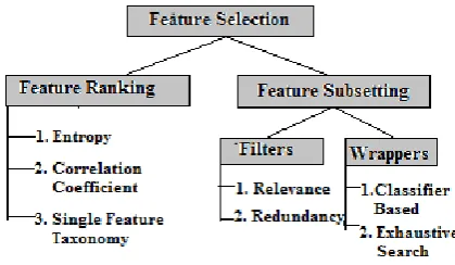
optimal subset. A brief survey on feature selection and various types of feature selection algorithms are depicted in figure 1.

Fig 1. Various existing Feature Selection Strategies

setting algorithms are nonspecific models and not intended to customize feature subsetting to extract one or two specific target class(es). Therefore we state that to the best of our knowledge the literature as on today shows that, no attempts are made towards developing a target class guided feature subsetting algorithm. As mentioned previously, to avoid Non deterministic Polynomial time required for finding optimal feature subset, we propose to eliminate features having maximum variance which is expected to minimize the variance in the target class. With respect to this objective of our proposed work, we could find in literature Xiaofei , et al, has contributed in developing a generic model to minimize variance using Laplacian Regularization[28]. Nevertheless our proposed work is exclusively deliberated for feature elimination by maximum variance considering one target class at a time. This reason also makes our proposed work novel.

3.

OUTLINE OF THE PROPOSED

WORK

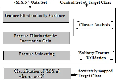
Selection of optimal features for the accurate extraction of a target class being the final objective, it is required to determine the optimal subset of features in a high dimensional space but exploring the combinations for subset of features will be impractical in high dimensional space. Hence, elimination of the unwanted features that do not contribute in extracting a target class is advocated before searching for subset of features. Determination of the optimal feature subset is dependent on the control set being provided to the proposed algorithm which describes the samples belonging to a target class. Thus, this work is restricted to only supervise feature sub setting. The sketch of proposed model is depicted in figure 2. Conventionally, when the features need to be eliminated there exists a problem of selecting the most undesired features for elimination.

To determine the most undesired features, scatter within the target class need to be measured which is statistically quantified by variance – a first order statistics. Higher the value of feature variance indicates that the samples are highly divergent from the mean showing a tendency to break away from a target class. Thus, at first stage such features are most preferred for elimination as they do not contribute in increasing the convergence of samples belonging to a target class and convergence of samples can be quantified as homogeneity. Number of similar samples classified under a target class is defined to be homogeneity. Hence, homogeneity is the desired property to be considered at the time of feature elimination because classification accuracy of a target class could be represented in terms of homogeneity which is explained in section 3.2.6 in detail. Although, elimination of features by maximum variance ensures homogeneity within a target class, it falls short in eliminating correlated features. Consequently at second stage, correlated features are eliminated based on both second order statistics

and information theory measure. Correlated features are identified based on both significant

correlation coefficient and mutual information between features. Since, the first two stages eliminate undesired

features, in the next level optimal subset of features is searched from the short listed features.

Fig 2. Block diagram of the proposed feature subsetting method to ensure lossless dimensionality reduction being

guided by a target class.

3.1

Feature Elimination

Since, the primary goal of this work is to find the optimal subset of features that can extract a target class accurately based on the knowledge provided; we need to select those features which can effectively represent and describe the specified class. In other words, the features which increase the non homogeneity of a target class influencing the divergence of the samples belonging to a target class are more preferred for elimination. The essential reason for the divergence of the samples is due to the variance caused by the features. Hence, they are said to be non-contributing features in the process of extraction of a target class. In conjunction with the elimination of non contributing features, it is also necessary to eliminate redundant features from the correlated features for the reason that one feature can always be inferenced in terms of other. As a result, feature elimination is carried out at two stages where first stage elimination is based on maximum variance and in second stage elimination is based both on correlation coefficient – a statistical measure and mutual information existing between features- information theory entropy.

3.1.1 Elimination of non-contributing features

based on variance

To standardize the range of features in the given data, the features are rescaled between [0, 1] using the normalization equation (1) so that all features get equal weight.

𝑓𝑠= _𝑓 𝑓𝑖−𝑓𝑚𝑖𝑛

the next section. All features whose variance is greater than the computed threshold value are preferred for elimination. But before elimination of such selected features, intra class distance is measured so that the comparison and validation can be performed on selected features. Intraclass distance is measured using Sum of Squared Error (SSE) as in equation (2). Analysis of variance is carried out to calculate SSE in order to verify the intraclass distance after feature elimination. SSE within a target class measures the variation of the individual observations about their group mean. The variance within a target class is minimized during elimination of undesired feature there by increasing the compactness.

𝑆𝑆𝐸 = 𝑓𝑖− 𝑓

2 𝑁

𝑓=1 (2)

Where, N - number of features 𝑓𝑖 - i th feature and 𝑓 - mean of all features. Given, a set of features {F} where, f € {F} and if var(f) is greater than threshold then, f is most preferred for elimination. The variance within the target class is measured using the equation (3)

𝑣𝑎𝑟 𝑓 = _𝑁1 𝑁𝑖=0 𝑓𝑖− 𝜇 2 (3)

where, 𝜇 = _𝑁1 𝑁𝑖=0𝑓𝑖 ;

3.1.2 Determination of threshold value for

variance

Threshold value for variance can be chosen heuristically akin to the work carried out by Nagabhushan, et. al, in 2004[6] who have chosen the threshold which is slightly greater than smallest variance from a single class that does not split the samples belonging to the same class. This method cannot significantly eliminate features when the dimensionality is very large like more than 200 in AVIRIS data set. Therefore, we propose to use decrease-and-conquer to find the threshold on variance that can play a significant role in the elimination of features with maximum variance effectively while satisfying the property of not splitting the samples belonging to the target class. In general, elimination of features should result in increased intra class cohesion at the same time should ensure that, no outlier exists. To validate this requirement during feature elimination, a target class as a cluster is analysed and interpreted as SSE as in equation (2). Algorithm to find threshold on variance is shown in figure4.

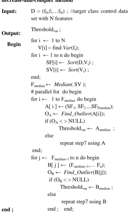
The prerequisite of using such a stringent rule in finding the threshold is due to the fact that, once all the features having variance greater than the threshold are eliminated they are not going to be backtracked next. Threshold should be chosen such that, the feature variance just above the threshold would result in another cluster. To accomplish this, we find median and then perform cluster analysis to find an outlier on left half of the median and right half of the median simultaneously. Figure3 depicts the decrease and conquer method used to find the threshold on variance. All the features whose variance greater than the threshold are eliminated.

Fig 3. Determination of threshold on variance using decrease-and-conquer method

Input:

Output: Begin

end ;

D = (f0,f1…fN) ; //target class control data set with N features

Thresholdvar ; for i ← 1 to N V[i]= find Var(fi); for i ← 1 to n do begin SF[i] ← Sort(D,Vi) ; SV[i] ← Sort(Vi) ; end;

Fmedian ← Median( SV ); # parallel for do begin for i ← 1 to Fmedian do begin A[ i ] ← (SF1, SF2 ,..SFFmedian); OA ← Find_Outlier(A[i]); if (OA < > NULL)

Thresholdvar ← Amedian ; else

repeat step7 using A end;

for j ← Fmedian+1 to n do begin B[ j ] ← (Fmedian+1,… Fn); OB ← Find_Outlier(B[j]); if (OB < > NULL) Thresholdvar ← Bmedian ; else

repeat step7 using B end ; end;

Fig 4.Algorithm to compute threshold on variance

3.2

Resolving the cutoff point in a

Dendrogram for feature validation

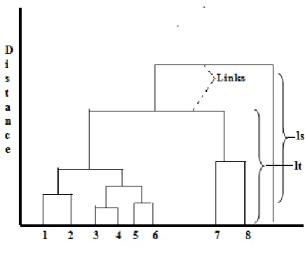
neighbouring links below it in the tree. A link that is approximately the same height as the links below it indicates that there are no distinct divisions. These links are said to exhibit a high level of stability. Nagabushan et al., [18] quantized it as a Stability Factor (4) and it is measured as in

equation (4).

Where ls is the current link height and lt represents the mean height of the links used for comparison in the dendrogram as shown in figure 5.

Fig 5. Stability factor in a dendrogram

In our work we have divided the stability factor by the standard deviation [17] as in equation (5).

𝑁𝑆𝐹 =𝑠𝑡𝑎𝑏𝑖𝑙𝑖𝑡𝑦 𝑓𝑎𝑐𝑡𝑜𝑟_𝜎

𝑙 (5)

Where, σl is the standard deviation of all the links used for comparison.

Normalized stability factor is computed by clustering the samples belonging to a target class using only the selected features. If appropriate features are selected then all the samples would form a single cluster due to lower proximity indicating no outlier. On the contradict part, if desired features are eliminated then there would exist an outlier in the cluster which is indicated through stability factor. Target class as a cluster is analysed and stability factor for every link is calculated. A ceiling stability factor from the calculated value is determined. If a desired feature is eliminated then a small increment in ceiling stability factor results in a outlier that indicates the incorrectness of the feature elimination.

3.3

Elimination of redundant features

Large number of features is produced at the time of data collection among which many are highly correlated or logically redundant. While some form of redundancy can be recognized at feature generation time, others can be identified by analyzing the data. Such surplus features if not handled

appropriately then they, become an over head at the time of mapping the target class. Hence, another primary goal of this research work is to detect which features are redundant or correlated for learning and exclude them.

To carry out the aforementioned task, the short listed features from first stage are considered and statistical characteristics in terms of redundancy is analysed. Redundant features are those which are highly correlated. Generally Pearson correlation coefficient is used to determine the correlation. If f1 & f2 are two features then Correlation coefficient r is calculated as in equation (5).

𝑟 = _{𝑛 𝑓1}𝑛 𝑓1𝑓2 − 𝑓1 𝑓2 _{2− 𝑓1 2}

𝑛 𝑓22_{− 𝑦} 2 (5)

But this metric has two limitations: first, it is suitable only if features are linearly correlated. Second, correlation coefficient based feature elimination leads to higher information loss. The reason for information loss is due to the approximation problem associated with correlation coefficient ‘r’ and probability of hypothesis testing ‘p’ for the given confidence interval. For an instance, with 95% confidence interval if r = > 0.5 then, it is approximated to 1 and considered to be positively correlated. But, if the features are eliminated by this approximation it may lead to loosing important target class relevant features and also may lead to inaccurate mapping of the target class. Hence, redundancy is estimated by calculating the Pearson correlation coefficient ‘r’ and significant redundant features are marked if its corresponding p-value is greater than or equal to 0.05. In order to eliminate all the redundant features from the marked list, the amount by which one feature can be inference by its redundant is quantitatively measured and in this paper it is termed as Inference Factor. For an instance, if feature f1 and f2 has p-value equal to 0.05 then, Inference Factor between f1 and f2 is computed and a feature with high inference factor is retained and its redundant is eliminated. Inference factor can be computed based on the entropy and joint entropy measure as explained next. Given a feature fi , entropy is calculated using equation (6)

𝐻 𝑓𝑖 = − 𝑛𝑖=1𝑃 𝑓𝑖 log2𝑃(𝑓𝑖) (6)

The entropy of feature fi after examining the feature fj is defined as joint entropy which is calculated as

𝐻 𝑓𝑖 = 𝑃 𝑓𝑓𝑗 𝑗 𝑃 𝑓𝑖 𝑓𝑗 𝑖

𝑗

𝑙𝑜𝑔2 𝑃 𝑓𝑖 ;𝑓𝑗

Where P(fi) is the prior probabilities of feature fi and P(fi/fj) is the conditional probabilities of fi when fj is known , for all the values of i and j. The elimination of feature fi if reduces the entropy of fi there by increasing the joint entropy 𝐻 𝑓𝑖 𝑓𝑗 then, it reflects the inference factor by fj about fi which can be expressed as in equation (7).

If 𝐼𝐹 𝑓𝑖 𝑓𝑗 is greater than 𝐼𝐹 𝑓𝑗 𝑓𝑖 then fj could be retained by eliminating feature fibecause fi can always be inference by fj.

Thus, the fusion of both the metrics namely Pearson correlation coefficient and Inference Factor expressed in terms of joint entropy can effectively handle redundant features within a target class there by alleviating the approximation problem involved in the process. It also avoids the problem of losing the features that contribute in mapping a target class. Hence, the proposed redundant feature elimination algorithm ensures minimum information loss so that, lossless dimensionality reduction by feature elimination with respect to target class can be effectively realized.

3.4

Feature subsetting

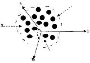
The above described two-stage feature elimination process eliminates the features that do not contribute in mapping a target class. As a result features space is reduced to n-feature space and if „n‟ is extremely small; finding the optimal subset of feature could be practically feasible. Otherwise, the subsetting algorithm requires further optimization. However, in this paper parametric feature subsetting algorithm is devised instead of optimizing the feature subsetting algorithm when the resulted d-feature space is further computationally challenging to handle. In this work we have assumed the parameter-P required by the process is the True Positive (TP) rate of a target class which is expected from the user. First few features are considered until the specified parameter is accomplished so that, time required for finding the optimal combination of features is minimized. On the other hand if n-feature space is extremely small then, wrapper based n-feature subsetting algorithm devised is as shown in figure6. The validation of the selected features is carried out which is based on number of samples classified under the target class. Let D = (f0,f1,...fN) is the original data set with N features and C= {c1, c2, ck} be the k-number of classes. Let OFS= {fs1,fs2,..fsn} be the optimal features selected when the proposed algorithm is adopted to map the target class TC such that, TC€ C. The advantage of the proposed algorithm can be observed in terms of three perspectives: i. Lossless dimensionality reduction by feature selection with respect to target class TC ii. Increase in the homogeneity within a target class could be realized which can be further utilized for compression iii. Possible accomplishment of higher feature reduction rate such that n<<N because, the devised feature selection algorithm is being guided only by a target class TC and remaining C-1 classes are being disregarded. Figure 7 and figure 8 depict the samples within a target class

Fig 6. Algorithm to find optimal subset of features

Fig 7. Scattered samples within target class before feature elimination in n-dimensional space

Fig 8. Increase in Intra Class Compactness and homogeneity after feature elimination in d-dimensional

space (d <<n) for target class input

output

begin

end; end;

D=(f0,f1,...fn)// target class control set with n features where,

n = N– (k+l) ; N = given N feature ;

k = features eliminated in first stage; l= features eliminated in second stage; {OFS}targetclass ; // Optimal subset of features found from lossless feature subsetting

for i← 1 to n for j ←1 to n {OFS}= fi ;

find J(fi) and J(fi,fj) ; //classification accuracy

if J(fi) > J(fi,fj)

{OFS}targetclass = fi ; else

3.5

Classification

Based on the multistage framework feature selection algorithm as described above, optimal features are generated. In the reduced feature space using the control set of a target class a minimum distance classifier is applied to verify the classification performance of target class and .The procedure for classification is shown in figure9. The number of samples classified under target class is analysed using F-Measure which estimate the homogeneity that exists within a target class. F-measure is the harmonic mean of Precision and Recall as shown in equation (8) that will range between 0 and 1. If it is larger, then true positive rate of the samples classified as target class is higher. The reason for choosing F-measure is that, harmonic mean of Precision and Recall is sensitive to outlier.

𝐹 = 2._𝑃+𝑅𝑃.𝑅 (8) where,

𝑃 = 𝑃𝑟𝑒𝑐𝑖𝑠𝑖𝑜𝑛 =_{𝑇𝑟𝑢𝑒 𝑃𝑜𝑠𝑖𝑡𝑖𝑣𝑒 +𝐹𝑎𝑙𝑠𝑒 𝑃𝑜𝑠𝑖𝑡𝑖𝑣𝑒}𝑇𝑟𝑢𝑒 𝑃𝑜𝑠𝑖𝑡𝑖𝑣𝑒

𝑅 = 𝑅𝑒𝑐𝑎𝑙𝑙 =_{𝑇𝑟𝑢𝑒 𝑃𝑜𝑠𝑖𝑡𝑖𝑣𝑒 +𝐹𝑎𝑙𝑠𝑒 𝑁𝑒𝑔𝑎𝑡𝑖𝑣𝑒}𝑇𝑟𝑢𝑒 𝑃𝑜𝑠𝑖𝑡𝑖𝑣𝑒

4.

EXPERIMENTS AND RESULTS

To demonstrate the effectiveness of the proposed target class based feature subsetting model, experiments are carried out on following three well known datasets. The first data set is extended IRIS data set consisting three classes, second data set is corn soyabean data set having two classes and the third data set is a hyperspectral remote sensed data which is a Indian Pine data set collected by Airborne Visible Infrared Imaging Spectrometer (AVIRIS) sensor. The experiments were conducted to select the optimal features that can effectively map target class using the knowledge available on the chosen data set. First experiment was conducted on IRIS and Cornsoyabean data sets since they are the well known benchmark data sets and hence, the correctness of the proposed algorithm can be demonstrated. However, to demonstrate the purpose of the proposed algorithm on high dimensional data, we also experimented on AVIRIS Indian Pine data set which is described in section 4.4.

4.1

Experiment I: Extended Iris data

To verify the operational feasibility and the correctness of the proposed feature elimination technique, IRIS - a benchmark data set is selected. It has 4 features x 150 samples, three classes with fifty samples per class. Extrapolation is usually used to create a tangent line with the two endpoints (x0, y0), (x1, y1) using a given point x. We have modified the extrapolation line equation (9) by adding and subtracting each feature with a unit number such that four features are extended to twelve features as shown in table1. For an instance, if f is the feature to be extrapolated then, f1= f + i and f0 =f - i, where i is the required unit distance between the extrapolated features.

𝑦 𝑥 = 𝑦0+ _𝑥𝑥−𝑥0

1−𝑥0 𝑦1− 𝑦0 (9)

To extrapolate the 4 features in IRIS data set, i value is chosen heuristically by observing the variation between two successive samples in the entire population. Consequently,

the observation on 150 samples shows that variation in feature1 is [0.1-0.3], feature2 is [0.1-0.3], feature3 is [0.1-0.1] and feature4 is [0.1-0.2]. Hence, i value for 4 features was approximately chosen as: if1:0.1, if2 :0.1 , if3 : 0.1 , if4: 0.05. By adopting linear extrapolation equation as explained above we get 12 features. Afterwards it is normalized using the formula (10). The chosen linear normalization formula ensures that, all the features are given equal weight because of their normalized values in the range [0, 1] and hence, all features participate without being ignored during the implementation of proposed algorithm.

fij=

fij−minj

maxj−minj

n j=1 m

i=1 (10)

4.1.1

Setosa as target class

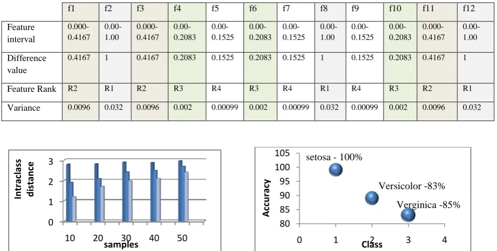
Setosa has less overlapping samples which is suitable as a target class to begin with the experiment. Feature elimination is carried out first based on variance and later based on redundancy. Since, all the features with maximum variance cannot be eliminated, threshold on variance was determined and all the features whose variance is greater than threshold were eliminated. Table3 shows the procedure adopted to calculate threshold on variance using 12 features. It shows that maximum the feature interval higher the feature variance. Threshold on variance was found to be 0.0049 based on decrease and conquer which is approximated to 0.004. Agglomerative clustering was applied to validate the threshold. No outlier was found with stability factor 1.547 but a small increment by 0.02 was forming two clusters which is not intended because already we know that all the samples belong to the same target class. So, we consider that cut off point as a threshold on variance. We found eight features having variance greater than threshold and they are the least desired features and hence got them eliminated.In the next stage, redundant features got eliminated based on redundancy and only two features were left out namely, ‘petal length’ & ‘petal width’. Since, finding the best subset out of two features was practically feasible, an optimal sub set was found by considering one feature at a time. This is similar to Sequential Floating Forward Selection [20] but specific to only Setosa class.

Table 1. Four features in IRIS data set extrapolated to twelve features

Features f1: petal length f2: petal width f3: sepal length f4: sepal width

Extrapolation f10= f1+0.1 f11= f1 - 0.1

f20=f2+0.01 f21=f2 - 0.01

f30=f1+0.05 f31=f1-0.051

f40=f1+0.1 f41=f1-0.1

Extrapolated features f10, f1, f11 f20 , f2, f21 f30, f1, f31 f40 , f1 , f41

Rearranged extrapolated features

f1 f2 f3 f4 f5 f6 f7 f8 f9 f10 f11 f12

Table 2 Threshold on variance calculated for Setosa as target class based on the decrease and conquer technique

f1 f2 f3 f4 f5 f6 f7 f8 f9 f10 f11 f12

Feature interval

0.000-0.4167

0.00-1.00

0.000-0.4167

0.00-0.2083

0.00-0.1525

0.00-0.2083

0.00-0.1525

0.00-1.00

0.00-0.1525

0.00-0.2083

0.000-0.4167

0.00-1.00

Difference value

0.4167 1 0.4167 0.2083 0.1525 0.2083 0.1525 1 0.1525 0.2083 0.4167 1

Feature Rank R2 R1 R2 R3 R4 R3 R4 R1 R4 R3 R2 R1

Variance 0.0096 0.032 0.0096 0.002 0.00099 0.002 0.00099 0.032 0.00099 0.002 0.0096 0.032

Graph 1. Validation of selected features for Setosa Graph2. Classification accuracy based on feature selected for target

4.1.2

Versicolor as target class:

Since, Versicolor has more overlapping samples with Verginica , we also tested the proposed algorithm considering versicolor as a target class . In the first stage five features were eliminated based on maximum variance and four redundant features were eliminated depending on inference factor in the second stage. Searching for the optimal subset was feasible because only three features were left out which resulted in six combinations, from which two features were selected as optimal. At each stage of feature selection, a validation was carried and it was observed that the elimination of undesired features for mapping a Versicolor class resulted in minimization of intraclass distance as depicted in graph 3. When the classification was performed using the obtained optimal features the target class was mapped with 90% accuracy as shown in graph 4. 53 samples were classified under the class verginica that includes fallaciously accepted samples. Similarly only 45 samples were classified under target class versicolor which has few false rejections.

This paper does not focus on handling the misclassification error which can be considered as a future work.

Graph3. Validation of selected features in Versicolor

0 1 2 3

10 20 30 40 50

In

tr

ac

lass

d

istan

ce

samples

80 85 90 95 100 105

0 1 2 3 4

A

cc

u

rac

y

Class

setosa - 100%

Versicolor -83%

Verginica -85%

0 2 4

10 20 30 40 50

In

tr

ac

lass

d

istan

ce

Graph 4. Classification accuracy based on feature selected for target class Versicolor

4.1.3

Verginica as target class:

Similar procedure was adopted to find the optimal subset of features as described above. „Petal length‟ & „Petal width‟ were found to be the optimal subset of features which is same as Versicolor. Graph 5 shows the validation results on selected features. Classification accuracy was found to be same as versicolor as depicted in graph 4. This experiment carried out on the benchmark data set indicates that, when feature selection is performed focusing one class at a time can drastically reduce the feature with an additional advantage of increasing the homogeneity within a target class. As a consequence, the homogeneity within a target class can be taken as an advantage for further compression in future.

Graph5. Validation of selected features of Verginica

4. 2 Experiment II: Corn Soyabean data set

The next experiment was carried out on another benchmark data set namely Corn Soya bean data set which has 62 samples X 24 features and 2 classes. Similar experiment was carried out by first considering Corn as the target class and next Soyabean as the target class separately.

When the proposed algorithm was probed for selecting the optimal features considering corn as a target class the following results were observed: 14 features were eliminated based on variance and 6 features were eliminated based on inference factor. Out of shortlisted four features only one feature was found to be optimal. The selected feature was validated and the result shows the minimization of intraclass distance as in graph5. Finally, all 62 samples were classified based on the optimal feature subset. The experiment conducted choosing soybean as a target class resulted in the selection of same feature as corn class. The validation and classification results are as same as in graph 6 and graph 7 respectively. This signifies that in few cases the proposed algorithm also behaves like conventional algorithm and hence dimensionality reduction cannot be claimed as lossy or lossless as experienced with IRIS data set.

Graph 6. Validation of selected features of target class corn from corn soyabean data set

Graph 7. Classification accuracy based on feature selected for target class Corn

Nevertheless, it provides an additional advantage of minimizing the intraclass distance and maximizing homogeneity within a target class so that further compression can be contemplated.

4.3

Experiment III: AVIRIS Indiana pines

To test the efficiency of the proposed model on high dimensional data which consists of more number of classes, we selected a well known hyperspectral data obtained from the AVIRIS imaging spectrometer for the scene Indiana Pines from North Indiana in 1992 taken on a NASA ER2 flight with a pixel size of 17m resolution [41].The Indiana pines data consists of 145X 145X220 bands of reflectance data with about two-thirds agriculture and one-third forest or other natural vegetation. There are two major dual lane highways, a rail line as well as some low density housing, small roads and other built structures. We have considered calibrated data which has a dimension of 145X145X200. Ground truth available is for sixteen classes as given in table 3 and figure 5 shows color coded ground truth.

4.3.1

Data pre-processing:

A three dimensional vector representation of the data was converted into a two dimensional vector format so that, further processing becomes easier. Therefore, 145X 145 X 200 vector was converted to 21025 X 200 2-D format.

For each band at each pixel in the entire scene, we have rescaled the data to range [0, 1] using the normalization equation (10).

Fig 5. Colour coded ground truth for Indiana Pine data set [41]

100%

90%

100%

85% 90% 95% 100% 105%

0 2 4

ac

cu

rac

y

Class

0 2 4 6

10 20 30 40 50

In

tr

ac

lass

D

istan

ce

Samples

0 5 10

5 10 15 20 25 30

In

tr

ac

lass

D

istan

ce

Samples

95 96 97 98 99

0 1 2 3

A

cc

u

rac

y

Class

TABEL 3. Ground truth for Indiana Pines data set

# Class Samples

1 Alfalfa 46

2 Corn-notill 1428

3 Corn-mintill 830

4 Corn 237

5 Grass-pasture 483

6 Grass-trees 730

7 Grass-pasture-mowed 28

8 Hay-windrowed 478

9 Oats 20

10 Soybean-notill 972

11 Soybean-mintill 2455

12 Soybean-clean 593

13 Wheat 205

14 Woods 1265

15 Buildings-Grass-Trees-Drives 386

16 Stone-Steel-Towers 93

4.3.2

Corn-mintill as a target class

In the conducted experiment on the high dimensional data Corn-mintill was chosen as a target class. The purpose of choosing Corn-mintill is as follows: a segment consisting of 122 pixels X 200 bands are chosen to design the control set. The threshold on variance is 0.048. At first stage 94 features were eliminated based on the variance. 80 features were found out to be correlated based on another metric called Pearson correlation coefficient. Using joint entropy, inference factor for the remaining 80 features was calculated. Subsequently, 40 features could be represented in terms of their redundant. Hence, those redundant features were eliminated. Totally 130 features were eliminated and 70 features selected for sub setting. 1-20, 110-140 and 171-192 feature range was shortlisted for subsetting. This also signifies that they are the contributing features for mapping corn-mintill. Comparatively 200:70 is a found to be effective feature elimination but information loss due to the eliminated features of a target class was unavoidable which would reflect in the accuracy of target class. Though, 200 fetures were reduced to 70 features even then finding the optimal subset was computationally challenging. Hence, to simplify and speed up the sub setting process we considered classification accuracy of the target class as the bounding criteria. To accomplish this, we heuristically fixed true positive (TP) rate as 95% and searched for first few features that can classify the 788 pixels as Corn-mintill out of 834 pixels. 38 features were found to be sufficient to give 95% TP of target class. So, remaining features were again eliminated and only 38 features were considered to design the control set of Corn-mintill. At each stage of feature elimination, validation was done on the selected features as shown in graph 8. The graph indicates the decrease in intra class distance by eliminating undesired features. This also increases homogeneity within a target class. It can also be observed that since, feature selection was carried out focusing only Corn-mintill as a target class, 200 features could be reduced to only 38 features by maintaining the TP rate as 95% which cannot be realized with general purpose dimensionality reduction.

Graph 8. Validation of selected features considering Corn-mintill as a target class

Eventually, when the selected 38 features were used to classify the entire population the target class mapped with 95 % accuracy where as few other classes like class 2 , class4, class 10, class 11 could also be mapped but with extremely less accuracy. But as mentioned earlier, the main objective of the proposed work is to select an optimal set of features that can accurately extract target class only. Hence, low classification performance of other classes is not an apprehension. Hence, we can claim that the proposed algorithm is a lossless dimensionality reduction with respect to target class and lossy with respect to other classe. Figure 7 show the part of results obtained with respect to the segmented data containing corn-mintill.

3 3 3 3 3 3 3 3 3 3 2 3 2 3 3 3 3 3 3 3 3 3 3 3 3 3 3 3 2 3 3 3 3 2 3 3 2 3 3 3 3 3 3 3 3 3 3 3 3 3 3 2 3 2 3 3 3 3 3 3 3 3 3 3 3 3 3 3 3 3 3 3 3 3 3 3 3 3 3 3 3 3 3 3 3 3 3 3 3 3 3 3 3 3 3 3 3 3 3 3 3 3 3 3 3 3 3 3 3 3 3 3 3 3 3 3 3 3 3 3 3 3 3 3 3 3 3 3 3 3 3 3 3 3 3 3 3 3 3 2 3 2 3 5 5 3 3 3 3 3 3 3 3 3 3 3 3 3 3 3 3 3 3 5 5 3 3 3 3 3 3 3 3 3 3 3 3 4 3 2 3 5 5 3 3 3 3 3 3 3 3 3 3 3 3 3 5 5 3 3 3 3 3 3 3 3 3 3 5 5 3 3 3 3 3 3 3 3 3 3 3 5 5 3 3 3 3 3 3 3 3 3 3 5 5 3 3 3 3 3 3 3 3 3 3 5 5 3 3 3 3 3 3 3 3 3 5 5 3 3 3 3 3 3 3 3 3 3 3 3 3 3 3

2 2 2 2 2 2 3 3 2 2 2 2 2 3 3 3 2 2 2 2 2 2 2 2 2 2 2 2 2 2 2 2 2 2 2 2 2 2 2 2 2 2 2 2 2 2 2 2

Fig 7. Segment of results obtained after the classification of 145X145 pixels using features selected for target class:

Corn-mintill .

4.4 Experiment IV: Exhaustive Search

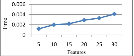
In this section an exhaustive search which searches for all best optimal subset is carried out in order to compare the performance of proposed algorithm. Given M number of features, an exhaustive search carried out to find best 2M possible subset was practically intractable. Considering setosa from IRIS data set as a target class an exhaustive search was carried to select the subset of features. Graph 9a & graph9b shows that as the number of features increases search time also increases but it was bound to polynomial time. The time complexity for exhaustive search is exponential time complexity: O(2N) where, N is the number of features.

0 20000 40000 60000 80000

122

In

tr

a

cla

ss

d

ista

n

ce

Further, the exhaustive search was carried out with AVIRIS Indian Pine data set taking Corn-mintill as a target class to find the best combination of features by varying features from 10 to 180. It was found that combinatorial process with 60 features and above was taking non polynomial time and the solution was intractable as shown in graph 9c. Consequently, in order to reduce the time required to find the optimal subset there is a necessity of feature elimination and in such cases methods like the proposed algorithm could be a best choice.

4.5. Experiment V: Sequential floating

forward selection (SFFS).

To demonstrate the effectiveness of customizing the dimensionality reduction, we also experimented with same data set using conventional sequential floating forward selection algorithm considering all the classes. The comparison of SFFS, exhaustive search and the summary of the proposed algorithm is shown in table 4.

Graph 9a. Exhaustive search on target class Setosa

Graph 9b. Exhaustive search on target class CornSoyabean

Graph 9c. Exhaustive search on target class AVIRIS Indian Pines

Table 4 . Performance comparison of proposed algorithm on three different data set with SFFS

SFFS Target class guided feature subsetting

algorithm

Target class Features

selected

Accuracy F-measure (average samples/ control set)

Feature s selected

Accuracy F-measure

( average samples/ control set)

Setosa: (Extended IRIS) 2 100% 0.6 1 100% 0.9

Versicolor: (Extended IRIS) 2 89% 0.49 2 89% 0.78

Corn: (Corn soyabean) 1 92% 0.67 1 92% 1.0

Soyabean:(corn soyabean) 1 94% 0.7 1 94% 0.95

Corn-mintill (AVIRIS Indiana Pines)

70 95% 0.4 38 95% 1.0

0 0.002 0.004 0.006

5 10 15 20 25 30

T

im

e

Features

0 0.002 0.004 0.006

5 10 15 20 25 30 35 40 45

T

im

e

Features

0 1000 2000

20 40 60 80 120 180

T

im

e

5. CONCLUSION AND FUTURE WORK

A customized dimensionality reduction by feature subsetting is proposed in this paper based on a target class. The results obtained conclude that if the optimal features are selected focusing only one target class at a time, then it gives better results in terms of reducing the dimensions compare to other supervised feature subsetting algorithms when classification is performed. The proposed technique eliminates the undesired features significantly so that intraclass variance is minimized and the optimal subset of features obtained is sufficient enough to represent a target class. Hence, classification accuracy of a target class is maximized which is as warranted by the application. However, with respect to other classes the accuracy is comparatively less which may not be important by the application.

So, this paper introduces a new strategy in dimensionality reduction as - lossless dimensionality reduction guided by a target class and lossy dimensionality reduction with respect to other classes while customizing the dimensionality reduction. Also, the results on the chosen data set reveal that, homogeneity within a target class is maximized.

This work leads to several future works. First, depending on the homogeneity within a target class spatial compression could be carried out. so that, further reduction in space be accomplishable. Second, transforming the original features or optimal subset of features in the future could minimize the information loss due to feature elimination. Third, optimization of the feature subsetting also needs to be carried out.

6. REFRENCES

[1] R. Duda, P. Hart, and D. Stork, Pattern Classification (2nd Edition): Wiley-Interscience, 2000.

[2] Nagabhushan . P. An efficient method for classifying remotely sensed data(incorporating dimensionality reduction). Ph.D thesis, University of Mysore, 1988. [3] Milliken, G. A., and D. E. Johnson, Analysis of Messy

Data, Volume 1: Designed Experiments, Chapman & Hall, 1992.

[4] Iffat A.Gheys, Leslie S.smith, Feature subset Selection in large dimensionality Domains, Pattern Recognition letters,31 May, 2009

[5] Yue Han, Lei Yu, A Variance Reduction Framework for Stable Feature Selection, International Conference on Data Mining, 2010 IEEE

[6] Lalitha Rangarajan , P.Nagabhushan, Content driven Dimensionality Reduction at block level in the design of an efficient classifier for spatial multispectral images , Pattern Recognition Letters, 23 September 2004

[7] Songyoot Nakariyakul, David P.Casasent, “An improvement on floating search algorithms for feature subset selection”, Pattern Recognition Letters, 42, 1932-1940, 2009

[8] Eugene Tuv, Alexander Borisov, George Runger, Feature Selection with Ensembles, Artificial Variables, and Redundancy Elimination, Journal of Machine Learning Research 10 (2009) 1341-1366

[9] Addenor Hacine-Gharbi, Phillipie Ravier, rachid Harba, Tayeb Mohamadi ,Low bias histogram-based estimation of mutual information for feature selection, Pattern recognition letters,10 March 2012

[10]Kulkarni Linqanagouda , P.Nagabhushan & K.Chidananda Gowda,a new approach for feature transformation to Euclidean space useful in the analysis of Multispectral Data,1994, IEEE

[11]P.Nagabhushan, K,Chidananda Gowda, Edwin Diday, “Dimensionality reduction of symbolic data, Pattern Recognition letters, 219-223, 1994

[12]Searle, S. R., F. M. Speed, and G. A. Milliken, "Population marginal means in the linear model: an alternative to least squares means," American Statistician,1980, pp. 216-221

[13]Chuan-Xian ren, Dao-Qing Dai, Bilinear Lancoz Components for fast dimensionality reduction and feature Selection, Pattern Recognition Letters, April 2010

[14]Vikas Sindhwani, Subrata Rakshit, Dipti Deodhare, Deniz Erdogmus,Jose .C.Principe, Partha Niyogi, “Feature Selection in MLPs and SVMs Based on Maximum Output Information” IEEE Transactions on Neural Networks, Vol.15. No 4. July 2004

[15]Thomas M.Cover, Joy A. Thomas, Elements of Information Theory, John Wiley & sons,1991

[16]Jaesung Lee, Dae-Won Kim, “Feature selection for multi-label Classification using multivariate mutual information”, Pattern Recognition Letters,34, 349-357,2013 summon

[17]Javier Grande, Maria Del Rosario Suarez , Jose Ramon Vinar, “A feature Selection Method Using a fuzzy mutual information Measure”, Innovation in Hybrid Intelligent systems, Springer-Verlag, ASC 44, 56-63 2007

[18]Lei Yu Huan Liu, Efficient Feature Selection via Analysis of Relevance and Redundancy, Journal of Machine Learning Research 5 (2004) 1205–1224 [19]Liangpei Zhang, , Lefei Zhang, Dacheng Tao, Xin

Huang, Tensor Discriminative Locality Alignment for Hyperspectral Image Spectral–Spatial Feature Extraction, 0196-2892,2012 IEEE

[20]Vasileios Ch Korfiatis, Pantelis A.Asvestas, Konstantinos K.Delibasis, “A classification system based on a new wrapper feature selection algorithm for diagnosis of primary and secondary polycythemia”, Computers in Biology and Medicine, 2118-2126,2013 [21]Eugene Tuv, Alexander Borisov, George Runger,

Fetaure selection with Ensembles , Artificial Variables and Redundancy Elimination, Journal of Machine Learning Research, 1341-1366,2009

[22]Annalisa Appice , Michelangelo Ceci, Redundant Feature Elimination for Multi-Class Problems, 21st International Conference on Machine Learning, Banff, Canada, 2004.

[23]Riccardo Leardi, Amparo Lupianez Gonzalez, “Genetic algorithms applied to feature selection in PLS regression: how and when to use them”, 0169-7439, 1998, Elsevier Science

Notes in Theoretical Computer Science 292, 135-151-2013

[25]Jun Zheng, Emma Regentova, Wavelet Based Feature Reduction Methods for Effective Classification of Hyper spectral Data, Proceedings of the International Conference on Information Technology: Computer and Communication, 0-7695-1916-4, IEEE ,2003

[26]Songyot nakariyakul, david P.Casasent, An improvement on floating search algorithms for feature subset selection, Pattern Recognition letters, 42, 1932-1940,2009

[27]Silvia Casado Yusta, “Different metaheuristic strategies to solve the feature selection problem”, Pattern Recognition Letters,30, 525-534,2009

[28]Xiaofei He, Ming Ji, Chiyuan Zhang, and Hujun Bao,A Variance Minimization Criterion to Feature Selection Using Laplacian Regularization, IEEE transactions on pattern analysis and machine intelligence, vol. 33, no. 10, october 2011 2013

[29]Zahn, C.T., "Graph-theoretical methods for detecting and describing Gestalt clusters," IEEE Transactions on Computers, C 20, pp. 68-86, 1971.

[30]Shuicheng Yan, Dong Xu, Benyu Zhang, Hong-Jiang Zhang, Qiang Yang, and Stephen Lin, “ Graph Embedding and Extensions: A General Framework for Dimensionality Reduction “ , IEEE ,0162-8828, 2007

[31]Muhammad Sohaib, Ihsan-ul-Haq, Qaisar Mushtaq.,Dimensionality Reduction of Hyperspectral Image Data Using Band Clustering and Selection Through K-Means Based on Statistical Characterstics of Band Images, International Journal of Advanced Computer Science, Vol2, No4 , 146-151, Apr 2012 [32]R. Pradeep Kumar, P.Nagabhushan., “Wavelength for

knowledge mining in Multi-dimensional Generic Databases, Thesis, university of Mysore, 2007

[33]Supriyanto, C. ; Yusof, N. ; Nurhadiono, B. ; Sukardi, "Two-level feature selection for naive bayes with kernel density estimation in question classification based on

Bloom's cognitive levels”,

Information Technology and Electrical Engineering, IEEE Conference Publications, 2013 , 237 - 241 [34]Yongkoo Han ; Kisung Park ; Young-Koo Lee

,“Confident wrapper-type semi-supervised feature selection using an ensemble classifier “,Artificial Intelligence, Management Science and Electronic Commerce , IEEE Conference Publications,2011 , 4581 - 4586