Forecasting Exchange Rates via Local Approximation Methods and Neural Networks

Munich Personal RePEc Archive

Forecasting Exchange-Rates via Local

Approximation Methods and Neural

Networks

Andreou, Andreas S. and Zombanakis, George A. and

Georgopoulos, E. F. and Likothanassis, S. D.

University of Patras, Bank of Greece, University of Patras,

University of Patras

December 1998

Forecasting Exchange-Rates via Local Approximation

Methods and Neural Networks

Andreou A. S.1

University of Patras,

Dept. of Computer Engineering & Informatics

and Artificial Intelligence Research Center

(U.P.A.I.R.C.)

Zombanakis G.A.2,*

Bank of Greece, Research Dept

Georgopoulos E. F.3

University of Patras,

Dept. of Computer Engineering & Informatics,

Artificial Intelligence Research Center

(U.P.A.I.R.C.)

and Computer Technology Institute

Likothanassis S. D.4

University of Patras,

Dept. of Computer Engineering & Informatics,

Artificial Intelligence Research Center

(U.P.A.I.R.C.)

and Computer Technology Institute

* Corresponding author

1.University of Patras, Dept. of Computer Engineering & Informatics, Artificial Intelligence Research

Center (U.P.A.I.R.C.), Patras 26500, Greece, tel.: +061 997755, fax: +061 997706, e-mail:

[email protected]

2. Bank of Greece, Research Dept., 21 Panepistimiou str., Athens 10250, Greece, tel.:+01 235809, fax:

+01 3233025, e-mail: [email protected]

3. University of Patras, Dept. of Computer Engineering & Informatics, Artificial Intelligence Research

Center (U.P.A.I.R.C.), Patras 26500, Greece, tel.: +061 997755, fax: +061 997706, Computer

Technology Institute, 3 Kolokotroni Street, Patras 26221 Greece, e-mail: [email protected]

4. University of Patras, Dept. of Computer Engineering & Informatics, Artificial Intelligence Research

Center (U.P.A.I.R.C.), Patras 26500, Greece,

Computer Technology Institute, 3 Kolokotroni Street, Patras 26221 Greece, tel.: +061 997755, fax:

Abstract

There has been an increased number of papers in the literature in recent years, applying several methods

and techniques for exchange - rate prediction. This paper focuses on the Greek drachma using daily

observations of the drachma rates against four major currencies, namely the U.S. Dollar (USD), the

Deutsche Mark (DM), the French Franc (FF) and the British Pound (GBP) for a period of 11 years,

aiming at forecasting their short-term course by applying local approximation methods based on both

chaotic analysis and neural networks.

1. Introduction

Predictability issues with special reference to stock and foreign-exchange markets seem

to attract increasing interest during the last few years. Concentration on forecasting

developments related to exchange rates, in particular, is not only justified by the

risk-versus-return tradeoff, but, in addition, by the fact that the exchange rate is often used as

policy instrument for tackling macroeconomic targets, like price stability or

balance-of-payments equilibrium. But even in cases in which the exchange-rate is allowed to

fluctuate in the international markets within margins that vary considerably depending

on the case, the fact remains that the various central banks retain the power to intervene

both in the domestic and international markets, manipulating the exchange-rate of their

respective currencies whenever the need arises. Such interventions are usually of drastic

nature, taking place either by foreign-exchange-reserves manipulation or by resorting to

interest rate policy, thus increasing the noise level which characterizes the behavior of

the time series involved. This issue introduces a considerable degree of difficulty when

it comes to forecasting, although, as Taylor (1995) points out, empirical evidence on the

The fact remains, however, that the relevant literature is full of cases in which

forecasting the exchange-rate of various currencies yields results which are either poor

(Marsh and Power, 1996; Pollock and Wilkie, 1996; West and Cho, 1995), or difficult

to interpret (Kim and Mo, 1995; Lewis, 1989). Some authors even conclude that there is

no such thing as best forecasting technique and the method chosen must depend on the

time horizon selected or the objectives of the policy-maker (Verrier, 1989). There are,

in addition, cases in which high persistence but no long range cycles have been reported

(Peters, 1994), something that leads to the conclusion that currencies are true Hurst

processes with infinite memory. On the other hand, long term dependence, supporting

that cycles do exist in exchange rates, has been found by other researchers (Booth et.

al., 1982, Cheung, 1993; Karytinos at. al., 1999). Despite various attempts to settle such

controversies (Pesaran and Potter, 1992), it is still not clear whether the source of the

dispute is, the differences with respect to sample size, noise level, pre-filtering

processes etc. of the various data sets employed, or the variety of tests that have been

used, or even a combination of these factors.

But the major problem associated with exchange-rate predictability has been indicated

by Meese and Rogoff (1983) and refers to the failure of the structural models to

outforecast the random walk model, due, among other things, to difficulties in modeling

expectations of the explanatory variables. The matter has attracted increasing attention

in the literature since then by authors like Leventakis (1987), De Grauwe et. al. (1993),

Frankel (1993), Baxter (1994) and Pilbeam (1995). Although all sources agree on the

empirical failure of models to forecast exchange-rate movements, none of them is able

them, however, seem to agree on the possibility that expectations are much more

complicated than what modern exchange-rate theories have specified (see e.g. Pilbeam,

1995), primarily because the rapid flow of information as well as the shift in the

demand and supply pattern bring about significant influence on the market movements

(Mehta, 1995). Thus several authors seem to conclude that even the forward rate, which

is considered very efficient when used to improve forecasting performance, can

sometimes fail in contributing towards this direction (e.g. Levich, 1989).

Turning to the case of the Greek drachma, attempts to forecast its exchange rates versus

major currencies are rather scarce. Karfakis (1991) has concentrated on the

drachma/USD exchange rate, while Koutmos and Theodosiou (1994) and Diamandides

and Kouretas (1996), have explored the predictability of the drachma rates with respect

to a number of European currencies, the USD and the Japanese yen. In all these cases,

however, the analysis is conducted in the context of exchange-rate models, with all the

drawbacks that such a choice might entail.

In face of the limited success of empirical literature to interpret exchange-rate

movements researchers have resorted, quoting Taylor (1995), to the use of “recently

developed sophisticated time-series techniques”. Indeed, one such technique is that

which relies on tracing chaotic behavior in the exchange-rates series examined, as well

as that of artificial neural networks. These, being data-driven approaches, have been

considered preferable to traditional, model-driven approaches used for forecasting

purposes, on the grounds of our earlier evaluation in the context of the literature cited.

In fact, exchange-rate literature has been recently enriched by an increasing number of

concerning exchange-rate forecasting compared to “conventional methods” (e.g. Mehta,

1995; Steurer, 1995; Refenes and Zaidi, 1995).

This paper uses both chaos theory and neural networks to predict the exchange rate of

four major currencies against the Greek Drachma, namely the U.S. Dollar (USD), the

Deutsche Mark (DM), the French Franc (FF) and the British Pound (GBP). Our primary

goal is to investigate the extent to which the time series involved exhibit chaotic

behavior, a prerequisite for applying the well known Farmer’s algorithm for prediction.

The results obtained on the basis of the application of Farmer’s algorithm will, at a

second round, be compared to the predictions obtained using another approach, namely

the emerging technology of artificial neural networks. Taking into account that so far

the results of research in this area have not established a general structural character of

currency markets, this analysis is expected to be useful for comparison purposes as

well. The results of both techniques are then compared focusing on the best prediction

performance.

1.1 Methodology and Data

Our time series consist of daily exchange rates of the four currencies already mentioned

against the Greek drachma. The rates are those determined during the daily “fixing”

sessions in the Bank of Greece. The data cover an 11-year period, from the 1st of

January 1985 to the 31st of December 1995, consisting of 2660 daily observations, a

population which is considered relatively small compared to that used in similar cases

in the natural sciences, but large enough compared to other studies in Economics and

Finance, in several of which the number of observations barely reaches 2000. The

in order to remove the trend. During the neural networks implementation, we used the

logarithmic data, so that results are directly comparable to those obtained using

Farmer’s algorithm. We also tested the predicting ability of neural networks when

incorporating the actual spot rates, since this option offers the advantage of not being

affected by the presence of trends or discontinuities in the series involved. Mehta

(1995), however, suggests avoidance of using the actual spot rates both because of the

non-stationary and quite random nature of this series and because of the daily

infinitecimal changes involved, something which reduces the learning ability of neural

networks. Taking these suggestions into account we have tackled this last problem by

rescaling our series in the range [0,1] in order to use the sigmoid activation function.

Our experiments showed that non-stationarity or randomness that can be observed

mainly by visual inspection did not affect learning and that forecasting results obtained

were highly satisfactory.

A final remark concerns the high jumps observed in the first 2 years (1985 and 1986) of

the series, immediately affected by the drachma devaluation. These samples were

excluded from the data library used in both Farmer and neural networks experiments,

characterized as outliers that correspond to significant level of noise. Other such spikes

observed scattered through the data series (e.g. 1992, 1993, 1995) were not removed

because they are low intensity and duration periods. Extensive simulations with both

methods showed that the course of forecasting was not affected by their presence.

The structure of this paper is as follows: Section 2 describes the leading role of the

exchange-rate policy in the context of an overview of the macroeconomic policies

analysis of the logarithmic data. Section 4 describes the methods and results of local

approximation forecasting on our data. The application of neural networks takes place

in section 5, while section 6 is devoted to a discussion on the economic interpretation of

the results. Finally, our conclusions are presented in section 7.

2. The Greek Environment

The exchange rate has been used as a major policy instrument in Greece since March

1975, when the drachma ceased to be pegged to the US dollar in terms of a fixed

exchange rate. The reasoning behind the extensive use of exchange-rate policy by the

authorities was based on its effectiveness thanks to its speed, flexibility and politically

costless action. This policy aimed at guaranteeing an acceptable level of price

competitiveness of Greek goods and services in the international markets and reducing the

balance of payments deficit. Since 1975 and until the early 90’s, however, the drachma

had been following a depreciating trend which, in parallel to the implementation of an

expansive monetary policy, has contributed to preserving high inflation rates (Bank of

Greece, 1984, p.31). In fact, for the time period under review, this policy has provided

for a devaluation in 1985 which resulted to the drachma depreciating by 16.3% in 1985,

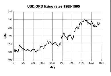
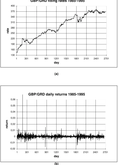
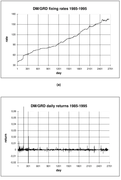
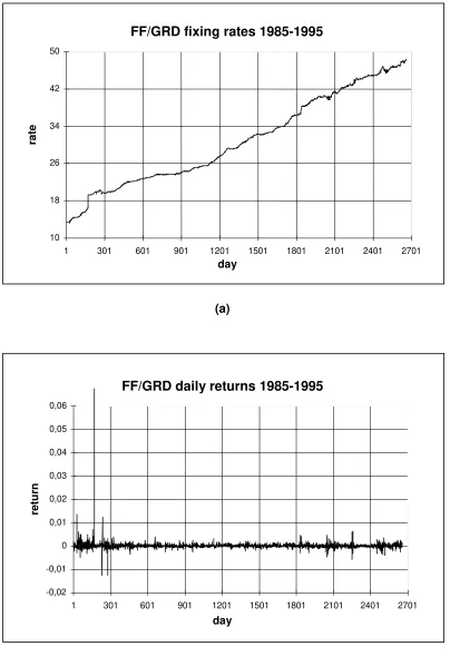
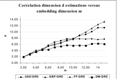
and 23.1% in 1986. This is shown by sharp peaks in Figures 1(b), 2(b), 3(b) and 4(b),

which, it is reminded, indicate the devaluation by just a daily sharp peak, since the

figures used are percentage changes of exchange rates rather than the currency rates

themselves. The beginning of the 90’s, however, introduces a dramatic policy change

with the authorities realizing the extent of the failure of this accommodating exchange

rate policy (Bank of Greece, 1986; Brissimis and Leventakis, 1989; Karadeloglou et. al.,

1998; Zombanakis, 1997). More specifically, this policy option proved to be rather

competitiveness of the Greek products in the international markets. The underlying

increased import penetration of the Greek economy due to the inability to resort to

structural changes in its production structure, is a supply-side problem, touching upon

issues like the application of the Marshall-Lerner condition and the existence of an

inverse J-curve effect characterizing the Greek economy (Karadeloglou, 1990). Thus,

the exchange rate policy during the mid-90’s changes to becoming “the hard - drachma

policy”, in the sense that the rate of depreciation does not fully accommodate the

inflationary gap between Greece and its trading partners. Additional intervention

measures have also been imposed in order to improve productivity, curtail production

costs, adjust the supply side to changes in demand, and face the impact of seasonal or

irregular factors on the drachma exchange rate. Concerning the drachma rates, the

depreciation versus the ECU declined to 4.1% for 1995 and 0.6% in 1996, acting as an

anti-inflationary policy instrument (Karadeloglou et. al., 1998) in anticipation of the

drachma participation with the ERM (Bank of Greece, 1995). This policy has proven to

be more than successful since, its drastic anti-inflationary impact was accompanied by a

significant interest-rate reduction representing a relief for the budget deficit and a decrease

of the capital cost of the business sector. Thanks, also, to the “hard-drachma”, increases in

servicing the currency denominated public debt have been avoided, the

foreign-exchange risk has been restricted, while the cost of the imported raw materials for Greek

export firms, the products of most of which bear a high import component, has been held

constant. Finally, the anti - inflationary effect of the “hard - drachma” policy has added to

the effort of attaining the price - stability target, a requirement for the country’s EMU

membership (Bank of Greece, 1994, 1997).1

1

As this policy undoubtedly provided for increased degree of discipline for the drachma

fluctuations versus the ECU participant currencies, it is natural to expect that the

predictability of the drachma/USD rate is reduced compared to that of the drachma rates

vis-à-vis the rest three currencies, due to the absence of any sort of relationship or

correspondence in terms of policy targeting between the drachma and the USD.

3. Statistical and Non-Linear Analysis

3.1 Statistical Description of the Data

The basic statistical properties and the logarithmic time series plots of the four data

series involved are listed in Table 1 and Figures 1(b), 2(b), 3(b) and 4(b). All series

have been characterized by strong skewness and kurtosis, while three out of four have

indicated absence of any significant autocorrelation, with the exception of the

DM/GRD, which has displayed first order autocorrelation and for which an AR(1)

specification has been employed. In general the statistical properties of all series are

rather similar in terms of distributional features something which is, to a large extent,

explained by the significance which the authorities have attributed to the drachma

exchange-rate versus major currencies as a policy instrument during the period under

consideration. It must be borne in mind that the data depicted in the graphs are first

differences of the logarithms of the original data, which makes it, in fact, percentage

changes. The interpretation of these diagrams, therefore, requires particular attention. In

Figures 1(b), 2(b), 3(b) and 4(b), for example, a devaluation will appear as a sharp peak

corresponding to just one daily observation, with the subsequent daily data dropping

3.2 Correlation and Generalized Dimensions

A number of measures of complex time series have been developed based on concepts

of non-linear dynamics. These include correlation dimension (Grassberger and

Procaccia, 1983; Tsonis, 1992) of the time series from the analyzed system, aiming at

distinguishing between chaoticity and randomness. The correlation dimension gives a

statistical measure of the geometry for the reconstructed attractor. In deterministic

chaotic systems the correlation dimension is frequently (but not always!) a fractional

number and is independent of the embedding dimension m, when m is large enough

(Schuster, 1988; Theiler, 1986). This work is not intended to provide for a complete

chaotic analysis of the series under study. Instead, we employ the dimension test, the

most popular among methods for revealing evidences of chaos, in order to use Farmer’s

algorithm, a technique which is proven to have very good results in predicting chaotic,

noise-free signals.

The procedure to calculate the correlation dimension requires constructing

time-delayed copies of the matrix:

ak=[ X(tk), X(tk+ô), Χ(tk+2τ),...,Χ(tk+(m-1)τ)] (1)

If the underlying state space of a system has d dimensions then the embedding space

needs to have 2d+1 dimensions to capture completely the dynamics of the system

(Takens, 1981). In practice we compute the correlation dimension using various

embedding dimensions m. The correlation dimension can be calculated from the

C (r) = 2

N N H(r-|a a

m 2 k j

k, j 1 N

−

∑

|) , ak≠aj (2)

where r is the radius of the located hyperspheres, |ak-aj| is the Euclidean distance

between the vectors ak and aj , N is the total number of elements of the signal and H is

the Heaviside function. The Heaviside function is equal to 1 if r ≥ |ak-aj| and is equal to

0 if r < |ak-aj|. The correlation dimension d(m) is expected to scale as a power of r, that

is (3)

0

r

,

r

(r)

C

∝

→

where d(m), the correlation dimension of embedding dimension m, can be estimated by

the slope of log(Cm(r)) versus log(r), i.e.

d(m) lnC (r) ln(r) r m ≡ → lim 0 ∂

∂ (4)

We work as follows : the plot of the slope of ∂lnC_m(r) /∂ln(r) versus ln(r), for r values

between 0.5 and 2, is constructed for each m. Correlation dimension d can then be

estimated directly from the slope versus ln(r) (Bountis at. al., 1993).

We expect d to vary with m until m reaches the level of 2d+1. Once this occurs, if the

system under study is not a random one, d saturates to a value called dsat and becomes

independent of m. Thus, dsat gives a fair estimate of the correlation dimension of our

system. For a truly random system d will constantly increase according to m because the

We calculated the correlation dimension for the four raw data series with the embedding

dimension ranging from m=2 to m=20 and τ=1 and the results were the following: DM

and FF showed a saturating dimension of approximately 6 and 8 respectively, while

USD and BP had their dimensions rising higher, at approximately 12 and 14

respectively, without showing any evidence of clear saturation (Figure 5). We also

tested DM using τ=2 (recalling the AR(1) correlation), but our results remained

practically the same. This result tends to show that the behavior of the drachma rates

versus the DM and FF is more disciplined, a fact which is absolutely justified by the

ERM membership of these two currencies, as well as by the orientation of the Greek

exchange-rate policy that uses the ECU as a guideline, in which the share of both

currencies together amounts to more than 50% .

Pre-filtered with AR(1), the DM series did not show any significant change in the

resulted dimension either. These results suggest that two of our series, DM and FF, can

be explained by determinism, however, a simple low-dimensional attractor is highly

unlikely. USD and GBP on the other hand seem to be more consistent with a random

explanation. Their dimension keeps rising almost like m which is a strong symptom of a

random behavior. Yet, we must be very cautious with the interpretation of these results

because of the small length in data series, which can lead to either an upward bias in the

case of chaotic data or to a downward bias in the case of random data (Ramsey and

Yuan, 1989;1990). Thus, we cannot rule out the possibility of a deterministic part in

USD and GBP signals, which may be perfectly covered by noise. We decided,

therefore, to apply Farmer’s algorithm to all four series, although only two of them (out

of four series) favored a (more) clear chaotic behavior, aiming at tracing further

of the predictive performance will then be feasible, confirming the deterministic or

stochastic explanation given above.

4. Local Approximation Forecasting - Farmer’s Algorithm

There has been a considerable number of papers in the literature, particularly during the

recent past, applying the methods and techniques of non-linear dynamics to forecasting

financial time series. Since the level of dimensionality (correlation dimension) provides

evidence that at least two of the series exhibit chaotic behavior, while the rest two are

either deterministic with a substantial amount of noise or just random, we use chaotic

dynamics and more specifically, Farmer’s algorithm, to predict the future course of our

time series.

According to this algorithm (Farmer and Sidorowich, 1987) predictions are made using

a local approximation approach as follows : first we embed our series in an

m-dimensional space, where m is suggested to be at minimum greater or equal to the

attractor’s dimension d, and produce the x-vectors shown in equation (1). To predict

x(t+T) we find the k nearest neighbours of x(t) that minimize the Euclidean metric ||.|| ,

let these be x(t’). From this point on, we have a variety of ways to construct the local

approximator. We can take k=1 (zero-order approximation) and xpred(t,T)=x(t’+T), or

let k vary, usually starting with k>m+1 for better results and then fit linear or

higher-order polynomials to the pairs (x(t’),x(t’+T)).

The accuracy of predictions is tested using the Normalized Root Mean Square Error

[

]

1

n_{i 1} xact(i) xn

n 2

σ_∆ =

− =

∑

[

]

RMSE(n)= x_pred(i)-x_act(i)

=

∑

If NRMSE=0 then predictions are perfect; NRMSE=1 indicates that prediction is no

better than taking xpred equal to the x-mean. We also test prediction with the correlation

coefficient r between the actual and predicted series.

As earlier stated, the application of Farmer’s algorithm to all four series aims at

distinguishing between the somewhat clear chaotic structure of the DM and FF series on

one hand, and the ambiguous behavior of the USD and the GBP on another. In fact in

the case in which the latter are truly random signals, then this method is expected to

result to a poor predictive performance. We run our tests with a rolling library, τ=1,

embedding dimensions m=6,8,..20 and neighbors k=1,3,5,8,10; we also calculated k=15

and k=17 for the USD and GBP series respectively, to be consistent with Farmer’s

recommendation for k>d+1. Tables 2-11 present an analytic report of the resulting

predictions for all series, including the pre-filtered DM one, summarized as exhibiting

low predictability, independently of the embedding dimension or number of nearest

neighbors used.

The results are summarized as follows:

USD/GRD

The e error ranged over 1 in nearly all experiments. The best performance was achieved

forecaster. Correlation coefficient results showed an approximately 28% follow-up of

the original series, for the same k and m values.

GBP/GRD

All simulations on the British Pound series exhibited worse results than the USD case.

The e error proved an inferior predictive performance compared to the mean forecaster,

as in all cases it stayed over 1. Correlation coefficient on the other hand resulted a better

predictive ability than e, following the jumps of the original series with a rather low

value of 28%, which cannot be regarded as a satisfactory forecasting performance. Best

performance was observed with k=5 and m=12.

FF/GRD

The results on the French Franc series show an improved forecasting ability compared

to the former two cases, which is justified by a relatively good e error and a mediocre

correlation coefficient. The former is slightly better than the simple mean, while the

latter indicates a 31% correlation between actual and predicted values. Best results were

obtained with k=8 and m=10.

DM/GRD

Similar predictive behavior was observed for both the returns and the AR(1) pre-filtered

returns of the DM series. A relatively good e error compared to the mean forecaster and

a correlation coefficient of 30%. The only difference was that the original return series

performed best with k=5 and m=16, while the residuals with k=8 and same m.

According to Farmer, we would expect better performance for a number of nearest

neighbors above the corresponding correlation dimension. This was confirmed only for

the FF and DM series. The fact that these currencies performed better than USD and

confirmation on the results regarding our systems’ structure produced in the previous

section.

In order to present a complete analytical framework, we repeated our calculations for

the same values of embedding dimension and nearest neighbors as before, but for

various library lengths, with more or less similar results. As a last attempt we tried

using an augmented or a standard library instead of a rolling one and once again our

results remained practically unchanged.

Following the orbit of the reconstructed attractor for each of the four data series we

found a number of false nearest neighbours, that is pseudo-neighbours, that belong to

another orbit than the one followed by the initial point selected, using the well-known

false neighbours test. The number of false neighbours was found to be for USD 273, for

GBP 374, for DM 32 and for FF 56. After removing these from each series we repeated

our calculations and found that the r coefficient for USD and GBP was just over 0.1 ,

while for DM it outperformed all previous results reaching 0.32. In the case of FF, it

stayed at the level of 0.26. The e error was not found to be improved for all currencies

involved.

Based on the above results our conclusions lead to rejecting the use of the specific

prediction algorithm for these four systems. Predictions made were limited to a success

level lower than 35%, which is most unsatisfactory. All series (including the pre-filtered

DM/GRD series) exhibited low predictions in every embedding dimension and any

predicting method for experimental data. This was more or less an expected result

mostly due to the high level of noise imposed on these systems.

5. Neural Networks Methodology

5.1 Neural Networks

This section is devoted to introducing and analyzing the technique of artificial neural

networks which belongs to a class of data driven approaches, as opposed to model

driven approaches. Certain general-purpose algorithms address the process of

constructing such a machine, based on available data. The problem is then reduced to

the computation of the weights of a feedforward network to accomplish a desired

input-output mapping and can be viewed as a high dimensional, non-linear system

identification problem. In a feedforward network, the units can be partitioned into

layers, with links from each unit in the kth layer being directed to each unit in the (k+1)th

layer. Inputs from the environment enter the first layer and outputs from the network are

manifested at the last layer. An m-d-1 architecture, shown in Figure 6, refers to a

network with m inputs, d nodes in the hidden layer and one node in the output layer.

We use such m-d-1 networks to learn and then predict the behavior of our time-series.

The hidden and output layers realize non-linear functions of the form:

(1 exp( )) (7)

1

1

+ − +

=

∑ w −

ixi i

m

Θ

where wi’s denote real valued weights of edges incident on a node, Θ denotes the

the previous layer. The well known Back Propagation (Rumelhart and McLelland,

1986) we used as a training algorithm.

5.2 System Design

From the given time series x={x(t): 1≤t≤N} we obtain two sets: a training set

xtrain={x(t): 1≤ t≤T}, and a test set xtest={x(t):(T+1)≤t≤N}, where N is the length of the

data record. The network is asked to predict the next value in the time sequence, thus

we have one output neuron. The number of inputs m is one of the most difficult

forecasting investigation aspects and it is examined during the simulations conducted.

The problem of the pattern selection strategy for neural networks training, the type of

which can be random and deterministic, has been presented comparatively in (Cachin,

1994). Simulation results show that convergence time and learning accuracy can be

improved using only deterministic type strategies, which is in fact what we do in our

experiments.

5.3 System Implementation, Training and Testing

The system described previously was implemented using a neural network

implementation tool, Cortex-Pro Neural Networks Development System (Unistat,

1994). As stated above, the momentum Error Back-Propagation was used to train the

networks minimizing the Mean Squared Error, having the learning rate equal to 0.2 and

the momentum term equal to 0.9. The initial values of the connection weights were

randomly selected in the interval [-1,1] using a uniform distribution. All simulations

“run” for 400 iterations during the learning phase (epochs), with the training samples

length set to 1200 and the testing ones to 300. Our predicting horizon is one sample

the high level of noise imposed, a fact that allows only for short-term forecasting

attempts.

The different networks implemented were trained using two transformed data sets, the

logarithmic set, used also in Farmer’s algorithm, to make possible a direct comparison

between the two methods and the raw price data, i.e. the actual (fixed) exchange of the

four currencies versus the Greek drachma (Figures 1(a), 2(a), 3(a) and 4(a)). The latter

did not undergo a de-trend procedure for two reasons: First because neural networks

belong to a class of mapping techniques that do not require such preprocessing and

second to investigate whether trend is a significant part of the information needed by a

network to generalize. As already mentioned, every data set used as input was first

rescaled to the range [0,1] which is required when using the sigmoid function (eq. 7).

The number of inputs was chosen to cover from a two days available information to

approximately one month (20 samples), after numerous simulations that showed that

when the past history fed into the networks was constituted with over one month’s daily

values the performance was worsen. The number of hidden neurons was also chosen

empirically. Because of the heuristic nature of this methodology we conducted our

experiments by trial and error, aiming at reaching convergence in time and performance

in logical bounds. The reported results were the best achieved.

5.4 Simulation Results

Tables 12 through 15 present those network architectures that performed best according

to the NRMSE and Correlation Coefficient error measures when using both the

errors were measured over the testing (out-of-sample) phase, that is, a set of data

excluded from the learning process.

The general conclusion we can derive is that the logarithmic returns exhibit poor

predictive behavior for all currencies involved, while untransformed raw prices show a

remarkably high and stable level of success. FF and DM produced more successful

predictions than USD and GBP, confirming the deterministic nature of their structure.

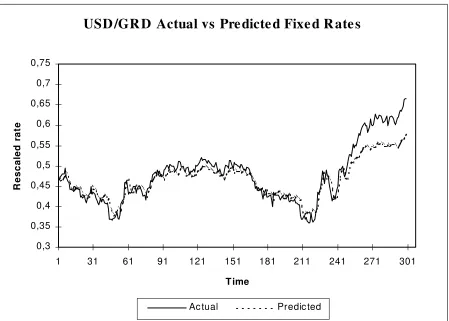
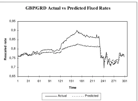
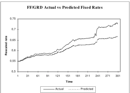
Figures 7 to 10 present graphically the results of the neural network architecture that

performed best in each raw price series.

Analytically:

USD/GRD

The return series proved a mediocre forecasting success, with correlation coefficient

reaching its highest value at approximately 26% and NRMSE slightly better than the

simple mean. The same results were observed when Farmer’s algorithm was employed,

thus none of the two methods seem to excel. The raw price input on the contrary

provided very good results, with almost 98% correlation between actual and predicted

series and a very low NRMSE of nearly 0.4 .

GBP/GRD

Identical with the Dollar, the GBP returns resulted a mediocre forecasting success, also

similar to the one obtained with Farmer’s algorithm, with a slight inferiority regarding

the correlation coefficient, which stays below 24%. The same picture is observed

regarding raw prices: very high level of correlation, over 98% and a quite low NRMSE

of nearly 0.6 .

Slightly better compared to the previous two cases is the performance of the FF

logarithmic series: correlation of 35% and NRMSE lower that the mean forecaster. No

significant diversification from Farmer’s performance though, which leads to conclude

a “draw” for the two methods. Following the stability of raw-price results, the networks

achieved high correlation, over 99%, and low NRMSE 0.6 .

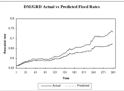
DM/GRD

The results reported for the DM series also follow the general setting established by the

previous cases: mediocre performance for the returns (both the simple and the

AR(1)-residuals), identical to Farmer’s NRMSE, but with a slightly lower correlation, and a

very successful forecasting behavior for the actual, untransformed prices, that reaches

over 99% correlation and 0.6 NRMSE.

6. Evaluation of results

In cases in which the input is in logarithmic form, both methods, that is Farmer’s

algorithm and neural networks, do not yield satisfactory results being, therefore, not

suitable for prediction purposes. The clear superiority of neural networks over Farmer’s

algorithm as a prediction tool is realised when it comes to using the actual,

untransformed rates. The presence of trend, which renders the predictive performance of

Farmer’s algorithm ineffective, seems to help the networks to embody all the available

information regarding the structure of all four currency series and thus produce highly

successful results. From an economist’s point of view, there should be no preference

favouring any particular sort of input type, provided that the prediction obtained is

successful. Any explanation, therefore, concerning the preponderance of the raw price

data over the first differences of their logarithmic transformations must take place in the

a daily basis, yields both positive and negative observations the mean value of which

centers around zero, something which does not allow the network to detect and learn a

particular pattern of behavior. The raw price data, on the contrary, help the network to

learn and generalize more efficiently, especially when it comes to short-term

forecasting, since they reveal not only the trend of the rate itself, but possibly, in

addition, the short-term expectations of the market. It is reminded at this point that

failing to incorporate the complexity of such expectations has been considered as one of

the major reasons why satisfactory exchange rate predictions are sometimes difficult to

achieve (Pilbeam, 1995).

Turning to the interpretation of the results obtained, these have been, to a considerable

extend, anticipated and lead to plausible conclusions as regards the degree of

determinism and predictability of the behavior of the drachma exchange-rate

fluctuations versus the four currencies involved.

Prediction seems to be more successful in the case of the DM and the FF drachma rates,

while that obtained in the case of the GBP and the USD rates appears to be slightly

inferior. This difference in forecasting performance is attributed to the nature of the

exchange-rate policy followed by the authorities during the period under consideration

and which has already been analyzed earlier in this paper. More specifically, targeting

the drachma rates with reference to the ECU in which the drachma as well as all other

currencies involved in this analysis participate, with the exception of the USD, leads to

expecting the corresponding drachma rates against the ECU - participant currencies to

be more easily predictable. It has been argued in the literature, in fact, that ECU

in cases like the rates of the DM and the FF which represent more than 50% of the total

ECU participation. In addition, the hard-drachma policy used as an anti-inflationary

device, provided for very low fluctuations for the rates of these three currencies versus

the Greek drachma, something which adds an element of discipline in the behavior of

these series, thus making their future course more predictable.

The increased predictability thanks to these low exchange-rate fluctuations has been

reinforced, particularly for the DM and the FF rates by their ERM participation for the

period under review. The bands within which the rates of the two currencies have been

allowed to fluctuate in the international markets contributed to their disciplined

behavior and, consequently, to the increased predictability associated with it.

The case of the GBP results seems to reinforce our line of argument: The GBP has

always been an ECU participant, whereas its ERM membership has been suspended on

the 16th of September, 1992. Predictions associated with the drachma rates versus the

GBP, therefore, are expected to be inferior compared to the DM and FF rates for the

same sample period, to the extent that its short ERM membership may count. Indeed the

prediction results obtained on the basis of the algorithms employed are very much in

accordance with the line of argument stated above.

Irrespective of the prediction performance regarding the drachma rates versus the

various currencies involved in this paper, one must point out that all four time series are

expected to be noise-polluted due to exogenous disturbances of two categories: Those

resulting form corrective measures taken by the authorities in order to offset possible

not necessarily of economic nature. Typical cases of the latter include the 1987 stock

market collapse, the German political and economic reunification in 1990 and the ERM

wider bands in 1993. Similar factors introducing noise on the drachma side may be

taken to be the 1985 devaluation, the prolonged pre-election period between 1989 and

1990 and the complete liberalization of capital movements in 1994.

It becomes obvious, therefore, that time series composed of empirical observations like

daily exchange rates are difficult to interpret and forecast and that minimizing the

presence of noise in such cases is a tedious task. The main problem arises because, as

earlier stated, these rates are to a significant extend affected by the interference of the

authorities in the framework of a predetermined exchange-rate policy. It has already

been pointed out in the introduction of this paper that Taylor (1995), in a

comprehensive survey on the issue of exchange rates, indicates the existence of

evidence concerning a link between official intervention and exchange-rate

predictability. What remains to be seen in this paper is the sort of link that exists when it

comes to the specific case of the Greek drachma versus the four currencies involved and

the extent to which the impact of the authorities’ interference is favorable or adverse.

An additional complication is introduced due to the choice of the particular sample

period, in the course of which both the logic and the extent of the government

intervention vary considerably. Thus, the beginning of the period under consideration is

characterized by generous depreciation rates, including a drachma devaluation, while

the beginning of the 90’s introduces the “non-accommodating” exchange-rate policy.

These complications suggest that future research should be undertaking focusing on the

the case of which the presence of noise is expected to be weaker. Once a successful

forecast for such rates has been realized, these rates may be used to derive drachma

cross-rates, on the basis of a preannounced government policy. This tactical move is

expected to avoid a considerable degree of noise and yield more reliable results.

7. Conclusions

This paper has focused on examining the degree of predictability of the Greek drachma

exchange rates with respect to four major currencies, using methods and techniques of

non-linear dynamics and neural networks and has resulted to the following main

conclusions:

1. The FF/GRD and DM/GRD time series exhibit chaotic behavior, with attractor

dimensions of approximately 8 and 6 respectively, while the USD/GRD and GBP/GRD

time series exhibit a more random behavior. Given these chaotic characteristics,

Farmer’s algorithm has been applied to test the prediction of all four series involved,

plus that of the pre-filtered DM/GRD. This exercise resulted in indicating that all time

series exhibit low predictions in every embedding dimension and any neighbour

number, with the level of the performed predictions being as low as about 30%, which

is obviously not satisfactory. Thus Farmer’s algorithm does not seem to be the most

suitable predicting method, for such experimental data, with high level of noise.

2. Simulations in the context of neural network methodology involving first differences

of logarithmic values were equally unsatisfactory to those obtained using Farmer’s

derived using as input the actual, untransformed exchange-rate figures. The networks

have been very successful in learning all exchange-rate series involved and thereby in

making accurate predictions.

3. The nature of the Greek economic policy which involves the determination of

drachma rates with reference to the ECU in which the DM, the FF and the GBP occupy

an overwhelmingly large percentage of the total currency participation, contributes to

the predictability of the exchange rates of these currencies versus the drachma. The

USD/GRD rates, on the contrary, seem to be tougher to predict, due to the absence of

any such link between the two currencies in terms of economic policy planning.

4. An additional element of discipline that concerns particularly the DM and the FF

and, to a much lesser extent, the GBP is related to the ERM membership of these

currencies. Indeed, restricting the fluctuations of these currencies in the international

markets within the ERM bands provides for increased discipline in the behavior of their

exchange-rates. This element of discipline adds to the predictability of the rates of these

currencies versus the drachma due to the reason analyzed in point 3 above.

5. A final point concerning the conclusions of this paper relates to the contribution of

government interference in the drachma rates prediction. More specifically, targeting

the exchange-rate policy with reference to the ECU in which the DM, the FF and the

GBP participate, the former two being, in addition, full ERM members for the period

under review, adds to the predictability of the exchange-rates of these currencies versus

the drachma. It seems, therefore, that, in what concerns drachma exchange rates against

these rates is not as unclear as it has been claimed in the literature.

REFERENCES

Bank of Greece, 1997, “Annual Monetary Program Announcement”, Athens.

Bank of Greece, 1984, “Report of the Governor”, Athens.

Bank of Greece, 1986, “Report of the Governor”, Athens.

Bank of Greece, 1994, “Report of the Governor”, Athens.

Bank of Greece, 1995, “Report of the governor”, Athens.

Bank of Greece, 1997, “Report of the governor”, Athens.

Baxter, M., 1994, “Real Exchange Rates and Real Interest Differentials”, Journal of

Monetary Economics 33, (1), 5-37, 1994.

Booth, G. G., F. R. Kaen, and P. E. Koveos, 1982, “R/S analysis of foreign exchange

rates under two international monetary regimes”, Journal of Monetary Economics 10,

407-415.

Bountis, T., L. Karakatsanis, G. Papaioannou and G. Pavlos, 1993, “Determinism and

noise in surface temperature time series”, Annales Geophysicae 11, 947-959.

Brissimis S.N. and J.A. Leventakis, 1989, “The Effectiveness of Devaluation: A

General Equilibrium Assessment with Reference to Greece”, Journal of Policy

Modeling 11(2), 247-271.

Cachin, C., 1994, “Pedagogical Pattern Selection Strategies”, Neural Network, 7, No.1,

175-181.

Cheung, Y. W., 1993, “Long Memory in Foreign-Exchange Rates”, Journal of Business

De Grauwe, P., H. Dewachter and M. Embrechts, 1993, “Exchange-Rate Theory”

(Blackwell, Oxford).

Diamandides, P. and G. Kouretas, 1996, “Exchange-Rate Determination: Empirical

Evidence for the Greek Drachma”, Managerial and Decision Economics 17, 277-290.

Farmer J. D. and J. J. Sidorowich, 1987, “Prediction Chaotic time series”, Physical

Review Letters 59, 845-848.

Frankel, J. A., 1993, “On Exchange Rates” (MIT Press).

Grassberger, P., and I. Procaccia, 1983, “Measuring the strangeness of a strange

attractor”, Physica D9, 189-208.

Hilborn, R. C., 1994, “Chaos and Nonlinear Dynamics - An Introduction for Scientists

and Engineers” (Oxford University Press).

Karadeloglou P., C. Papazoglou, G. A. Zombanakis, 1998, “Is the Exchange Rate An

Effective Anti-Inflationary Policy Instrument?”, Economia.2(1), 47-72.

Karadeloglou, P., 1990, “On the existence of an inverse j-curve”, Greek Economic

Review 12, 285-305.

Karfakis, C., 1991, “A Model of Exchange-Rate Policy: Evidence for the US Dollar -

Greek Drachma Rate 1975 - 1987”, Applied Economics 23, 815-820.

Karytinos A., Andreou, A.S. and Pavlides G., 1999, “Long-Term Dependence in

Exchange Rates”, Journal of Discrete Dynamics in Nature and Society.

Kim, J. C. B. and S. Mo, 1995, “Cointegration and the long-run forecast of exchange

rates”, Economic Letters 48, 353-359.

Koutmos, G. and P. Theodossiou, 1994, “Time-Series Properties and Predictability of

Greek Exchange Rates”, Managerial and Decision Economics 15, 159-167.

Archiv 123, 363-376.

Levich, R., 1989, “Forward Rates as the Optimal Future Spot Rate Forecast” (in C. Dunis

and M. Feeny Exchange-Rate Forecastng, Probus, Chicago).

Lewis, K. K., 1989, “Can learning affect exchange-rate behavior? The case of the Dollar

in the early 1980’s”, Journal of Monetary Economics 23, 79-100.

Marsh, I. W. And D. M. Power, 1996, “A note on the performance of foreign exchange

forecasters in a portfolio framework”, Journal of Banking & Finance 20, 605-613.

Medio, A., 1992, “Chaotic Dynamics - Theory and Applications to Economics”

(Cambridge University Press).

Meese, R. and K. Rogoff, 1983, “Empirical Exchange-Rate Models of the Seventies”,

Journal of International Economics 14, 3-24.

Mehta, M., 1995, “Foreign-Exchange Markets” (in Refenes A.P. (ed.) Neural Networks

in the Capital Markets, Wiley, U.K.).

Pawelzik, K. And H. Schuster, 1987, “Generalized dimensions and entropies from a

measured time series”, Physical Review A35, No 1, 481-484.

Pesaran, H. M. and S. M. Potter, 1992, “Nonlinear dynamics and econometrics: An

introduction”, Journal of Applied Econometrics. 7, s1-s7.

Peters, E. E., 1994, “Fractal Market Analysis - Applying Chaos Theory to Investment

and Economics” (Wiley Finance Edition).

Pilbeam, K., 1995, “Exchange-Rate Models and Exchange-Rate Expectations: An

Empirical Investigation”, Applied Economics 27, 1009-1015.

Pollock, A. C. And M. E. Wilkie, 1996, “The quality of bank forecasts: The dollar-pound

exchange rate 1990-1993”, European Journal of Operational Research 91, 306-314.

Ramsey, J. B. And H. J. Yuan, 1989, “Bias and error bars in dimension calculations and

Ramsey, J. B. And H. J. Yuan, 1990, “The statistical properties of dimension calculations

using small data sets”, Nonlinearity 3, 155-176.

Refenes, A. P. and A. Zaidi, 1995, “Managing Exchange-Rate Prediction Strategies with

Neural Networks” (in Refenes A.P. (ed.) Neural Networks in the Capital Markets,

Wiley, U.K.).

Rumelhart, D. E. and J. McLelland, 1986, “Parallel Distributed Processing”, (Cambridge,

MA, MIT Press).

Schuster, H., 1988, “Deterministic Chaos” 2nd ed. (Physik-Verlag, Weinheim).

Schwarz, G., 1978, “Estimating the dimension of a model”, Annals of Statistics 6,

461-464.

Six, J. M., 1989, “Economics and Exchange-Rate Forecasting” (in C. Dunis and M.

Feeny Exchange –Rate Forecastng, Probus, Chicago).

Steurer, E., 1995, “Non-Linear Modeling of the DEM/USD Exchange Rate” (in Refenes

A.P. (ed.) Neural Networks in the Capital Markets, Wiley, U.K.).

Takens, F., 1981, in Dynamical Systems and Turbulence. Vol. 898 of Lecture Notes in

Mathematics, Rand and Young eds. (Springer-Verlag, Berlin).

Taylor M.. P., 1995, “The Economics of Exchange Rates”, Journal of Economic

Literature XXXIII, 13-47.

Theiler, J., 1986, “Spurious dimension from correlation algorithms applied to limited

time-series data”, Phys. Rev. A34, 2427-2432.

Tsonis, A., 1992, “Chaos : From Theory to Applications” (Plenum, New York).

Unistat Ltd, 1994, Cortex-Pro Neural Networks Development System, London, U.K.

Verrier, M., 1989, “Selection & Application of Currency Forecasts (in C. Dunis & M.,

Feeny (eds.), Exchange-Rate Forecasting, Probus, Chicago, USA), 303-343.

volatility”, Journal of Econometrics 69, 367-391.

Zombanakis G. A., 1997, “Is The Greek Exporters’ Price Policy Asymmetric?”, Greek

Economic Review, 19 (2).

LEGENDS FOR FIGURES

Figure 1: USD/GRD time series plots: (a) Daily fixed-rates, (b) Daily returns

Figure 2: GBP/GRD time series plots: (a) Daily fixed-rates, (b) Daily returns

Figure 3: DM/GRD time series plots: (a) Daily fixed-rates, (b) Daily returns

Figure 4: FF/GRD time series plots: (a) Daily fixed-rates, (b) Daily returns

Figure 5: Correlation dimension estimates versus embedding dimension for the

USD/GRD, USD/GRD, DM/GRD and FF/GRD series of returns.

Figure 6: The m-input, d-hidden nodes and 1-output MLP neural network architecture.

Figure 7: Actual values versus neural network predictions of the USD/GRD fixed rates

series using a 6-5-1 MLP architecture.

Figure 8: Actual values versus neural network predictions of the GBP/GRD fixed rates

series using a 2-5-1 MLP architecture.

Figure 9: Actual values versus neural network predictions of the FF/GRD fixed rates

series using a 2-3-1 MLP architecture.

Figure 10: Actual values versus neural network predictions of the DM/GRD fixed rates

USD/GRD fixing rates 1985-1995

100 130 160 190 220 250 280

1 301 601 901 1201 1501 1801 2101 2401 2701

day

rat

e

(a)

USD/GRD daily returns 1985-1995

-0,02 -0,01 0 0,01 0,02 0,03 0,04 0,05 0,06

1 301 601 901 1201 1501 1801 2101 2401 2701

day

ret

u

rn

GBP/GRD fixing rates 1985-1995

130 160 190 220 250 280 310 340 370 400

1 301 601 901 1201 1501 1801 2101 2401 2701

day

rat

e

(a)

GBP/GRD daily returns 1985-1995

-0,02 -0,01 0 0,01 0,02 0,03 0,04 0,05 0,06

1 301 601 901 1201 1501 1801 2101 2401 2701

day

ret

u

rn

(b)

DM/GRD fixing rates 1985-1995

30 60 90 120 150 180

1 301 601 901 1201 1501 1801 2101 2401 2701

day

rat

e

(a)

DM/GRD daily returns 1985-1995

-0,02 -0,01 0 0,01 0,02 0,03 0,04 0,05 0,06

1 301 601 901 1201 1501 1801 2101 2401 2701

day

ret

u

rn

(b)

FF/GRD fixing rates 1985-1995

10 18 26 34 42 50

1 301 601 901 1201 1501 1801 2101 2401 2701

day

rat

e

(a)

FF/GRD daily returns 1985-1995

-0,02 -0,01 0 0,01 0,02 0,03 0,04 0,05 0,06

1 301 601 901 1201 1501 1801 2101 2401 2701

day

ret

u

rn

(b)

C orrelation dimension d estimations versus embedding dimension m

0,00 2,00 4,00 6,00 8,00 10,00 12,00 14,00

2,00 4,00 6,00 8,00 10,00 12,00 14

m

d

US D/GRD GBP /GRD FF/GRD DM /GRD

x t-1

x t-2

x t-m

Input Layer

Hidden Layer

Output Layer .

. . .

.

. .

. .

xt

hd

h3

h2

h1

USD /GR D Actual vs Pre dicte d Fixe d R ate s

0,3 0,35 0,4 0,45 0,5 0,55 0,6 0,65 0,7 0,75

1 31 61 91 121 151 181 211 241 271 301

T ime

R

esc

al

ed

r

at

e

Ac tual Predic ted

GBP/GRD Actual vs Predicted Fixed Rates

0,65 0,7 0,75 0,8 0,85 0,9 0,95

1 31 61 91 121 151 181 211 241 271 301

Time

R

esca

led

r

a

te

Actual Predicted

FF/GR D Actual vs Pre dicte d Fixe d R ate s

0,5 0,55 0,6 0,65 0,7 0,75

1 31 61 91 121 151 181 211 241 271 301

Time

R

escal

e

d

r

at

e

Ac tual Predic ted

Figure 9

DM /GRD Actual vs Predicted Fixed Rates

0,55 0,6 0,65 0,7 0,75 0,8

1 31 61 91 121 151 181 211 241 271 301

Time

R

es

cal

ed

r

at

e

Actual Predicted