Sparse Signals Reconstruction Via Adaptive Iterative
Greedy Algorithm
Ahmed Aziz
CS Dept.,Fac. of computers and Informatics Univ. of Benha
Benha, Egypt
Ahmed Salim
Mathematics Dept.,Fac. of Science Univ. of Zagazig
Zagazig, Egypt
Walid Osamy
CS Dept.,Fac. of computers and Informatics Univ. of Benha
Benha, Egypt
ABSTRACT
Compressive sensing(CS) is an emerging research field that has applications in signal processing, error correction, medical imaging, seismology, and many more other areas. CS promises to efficiently reconstruct a sparse signal vector via a much smaller number of linear measurements than its dimension. In order to improve CS reconstruction performance, this paper present a novel reconstruction greedy algorithm called the Enhanced Orthogonal Matching Pursuit (E-OMP). E-OMP falls into the general category of Two Stage Thresholding(TST)-type algorithms where it consists of consecutive forward and backward stages. During the forward stage, E-OMP depends on solving the least square problem to select columns from the measurement matrix. Furthermore, E-OMP uses a simple backtracking step to detect the previous chosen columns accuracy and then remove the false columns at each time. From simulations it is observed that E-OMP improve the reconstruction performance better than Orthogonal Matching Pursuit (OMP) and Regularized OMP (ROMP).
General Terms:
Signal reconstruction, Signal processing
Keywords:
Compressed sensing, Forward-backward search, Sparse signal reconstruction, Greedy algorithms
1. INTRODUCTION
Exploiting the sparse nature of the signals is one of the most important problems in various signal processing applications such as signal compression, inverse problems and the newly developed Compressive Sensing (CS)[1] approach. CS is a new theory of sampling in many applications, such as data network, sensor network [2], digital image and video camera, medical systems and analog-to-digital convertors [3]. CS technique is employed by directly acquiring a compressed signal representation of lengthM
for a lengthNsignal withM < N, which aims to measure sparse and compressible signals at a rate significantly below the Nyquist rate. For a one-dimensional real-valued discrete-time signalx ∈
RNof length N with S << N, where S is nonzero entries or sparsity level of the signal x, CS framework considers to reconstruction the signalxfrom the incomplete measurements.
y= Φx (1)
where y is anM ×1 vector with M < N and Φ represents
M×N sampling matrix. SinceM < N, the reconstruction ofx
fromyis generally ill-posed. However, Cands [4, 5] and Donoho’s [1, 6] work states that if x is sparse enough, in the sense that there are very limitedSnon-zero components inx, then the exact reconstruction is possible andxcan be well reconstructed from onlyM ≤O(Slog(N/S))measurements by reformulates Eq.(1) as a sparsity-promoting optimization problem
x=arg minkxk0 subject to y= Φx (2)
wherekxk0, called the normL0by abuse of terminology, denotes the number of nonzero elements inx. There are two families can be alternatively used to solve Eq.(2). One is the basic pursuit that is a convex relaxation leading to the norm minimization L1 in which replace theL0minimization in Eq.(2) with its closest convex approximation, the L1 minimization. Several different schemes have been proposed for solving theL1minimization such as using Linear Programming (LP)problem[7]. Although,L1 optimization methods could be used to solve the reconstruction problem, the computational cost is high enough, which makes them impractical for most CS applications.
This paper proposes a new iterative greedy algorithm , called Enhanced Orthogonal Matching Pursuit (E-OMP) for signal reconstruction. E-OMP employs forward selection and backward removal steps which iteratively expand and shrink the support estimate of the original data. E-OMP can operate both in the noiseless and noisy regime, allowing for exact and approximate signal recovery, respectively.
The rest of the paper is organized as follows: Section 2 briefly review related work. Problem descriptions and motivation are presented in section 3. Section 4 introduces E-OMP algorithm to carry out the proposed problem. The simulation of E-OMP algorithm is presented in section 5. In section 6, we conclude our work.
2. RELATED RESEARCH
During the past few years Compressive Sensing signal reconstruction problem has attracted a lot of attention from the research community. The work presented in this paper has been inspired by various existing research efforts. Historically, Matching Pursuit (MP) [8] is the first greedy pursuit. MP expands the support setT (the set of columns selected fromΦfor representingy) of
xby the dictionary atom, i.e. columns of the dictionaryΦwhich has the highest inner-product with the residue at each iteration. Major drawback of MP is that it does not take into account the non-orthogonality of the dictionary, which results in suboptimal choices of the nonzero coefficients.
The non-orthogonality of dictionary atoms is taken into account by the Orthogonal Matching Pursuit (OMP) [9]. OMP applies the greedy algorithm to pick the columns ofΦby finding the largest correlation betweenΦ and the residual ofy, this process called Forward step. At each iteration, one coordinate for the support of the signalxis calculated. Hopefully afterKiterations, the entire support of the signalxwill be identified.
Recently, more sophisticated pursuit methods, which select multiple columns per iteration, have appeared. For example Stagewise OMP, or StOMP [14] which selects in each step all columns whose inner-products with the residue is higher than an adaptive threshold depending on theL2 norm of the residue, using a rule inspired by ideas from wireless communications. StOMP is faster than OMP because of the selection rule, and it sometimes provides good performance, although parameter tuning can be difficult. There are no rigorous results available for StOMP. Alternatively, Needell and Vershynin developed and analyzed another greedy approach, called Regularized OMP, or ROMP [13]. ROMP groups inner-products with similar magnitudes into sets at each iteration and selects the set with maximum energy.
Compressive Sampling Matching Pursuit (CoSaMP) [10] and Subspace Pursuit (SP) [11] combine selection of multiple columns per iteration(forward step) with a backtracking step. At each iteration, these first expand the selected support by addition of new columns, and then prune it to retain only the best S
atoms(backtracking step). While SP/CoSaMP methods improve the performance of OMP method, they require the sparsity level S to be known for reconstruction. However, in most practical applications,this information could not be known before reconstruction. One way out is to guess the value of S before reconstruction. However, using an incorrectly estimated S, the performance will degrade quickly [16].
Iterative Hard Thresholding (IHT) [17] employs an iterative gradient search that first updates the sparse estimate in the direction of the gradient of the residue and then prunes the solution by either thresholding or keeping only theSlargest entries. A recent
IHT variant, Nesterov Iterative Hard Thresholding (NIHT) [18] employs Nesterovs proximal gradient [19] to update the sparse representation. NIHT provides no a priori performance guarantee, but still an online performance guarantee.
Like OMP/StOMP methods, E-OMP acts a stage by stage estimation of the true support set. Furthermore, similar to SP/CoSaMP methods, it uses a simple backtracking step to detect the previous chosen columns’ reliability and then remove the unreliable atoms at each time.
However, unlike most of the OMP-type methods, the first step of E-OMP method is to start by solving a least-squares problem and select only the columns of Φ that have the largest entries in this least-squares signal approximation. Furthermore, unlike SP/CoSaMP methods E-OMP method can achieve the blind sparse reconstruction without knowing the sparsity level S a priori. Besides, E-OMP adaptively chooses the forward and backward size depended onMrather than sparsity levelSlike SP/CoSaMP. The used notations in the following sections are given in Table 1.
3. PROBLEM DESCRIPTIONS
In this section, some space is devoted to a short overview of OMP which is important for the proposed algorithm because of their resemblance to the E-OMP algorithm and then the problem of OMP algorithm is described. Finally, paper motivation to solve this problem is proposed.
OMP is a forward algorithm which builds up an approximation one step at a time by making locally optimal choices at each step. At iterationk, OMP appendsT with the index of the dictionary atom closest tork−1, i.e. it selects the index of the largest magnitude entry of:
C= Φ∗rk−1
(3)
T =T∪C (4)
The projection coefficients are computed by the orthogonal projection:
W = Φ†Ty (5)
At the end of each iteration, the residue is updated as
rk=y−ΦTW (6)
These steps are repeated until a halting criterion is satisfied (the number of iterations=S). After termination,TandWcontains the support and the corresponding nonzero entries ofx, respectively. For more clarity and to illustrate OMP problem, consider the following simple example:
Φ =
1 1 0 1 1 0 1 0 0 1 0 1
, x=
0 1 1
, y=
1 1 0 1
, S= 2
wherey = Φx, Φ ∈ RM×N, x ∈ RN,y ∈ RM and S non zero components. Given a sensing matrix Φand an observation vector y, find the best solution toy = Φxwith at mostS non zero components.
By applying OMP algorithm with the following initialization parameters to solvey= Φx.
r0=y=
1 1 0 1
Table 1. : E-OMP Algorithm Notations
Symbol M eaning
S none zero components (sparsity level) k.kp the usualLpvector norm
Φ measurement matrix
u a positive integer
T estimated support set
rK the residue after thek0thiteration
x the target signal
xu restrictingxto itsulargest-magnitude components
W a projection coefficients set
∗ stands for matrix transposition
C a set which includes the largest magnitude entry ofΦ∗rK−1
x|T the restriction of the signalxto the setT
ΦT the column submatrix ofΦwhose columns are listed in the setT
Φ† the pseudo inverse of a tall, full-rank matrixΦand it expressed as(Φ†= (Φ∗Φ)−1Φ∗
)
E sparse approximation solution
H candidate set
F least-squares signal approximation set
Kmax maximum number of itreations
β termination parameter
ξ Forward step size(ξ=M/2)
ρ backward step size(ρ=ξ−M/3)
At iteration k = 1, OMP appends T with the index of the dictionary atom closest tork−1, i.e. it selects the index of the largest magnitude entry of:
C= Φ∗rk−1=
1 1 1 1 1 1 0 0 0 0 0 1
1 1 0 1 = 3 2 1
Therefore, the index of the first column will be added to the set
T (false column selection by OMP), since it is the index of the largest magnitude entry of C. Then OMP forms a new signal approximation by solving a least-square problem:
W= Φ†1y= (Φ∗1Φ1)−1Φ∗1y
=
( 1 1 1 1 ) 1 1 1 1 −1
( 1 1 1 1 )
1 1 0 1
= 0.7500
Finally, OMP updates the residual
r1=y−Φ
TW = 1 1 0 1
−0.7500 1 1 1 1 =
0.25 0.25
−0.75 0.25
During the next iterations, the OMP algorithm will add the second column index to setT.
From the previous example it is noticed that, at the first iteration, OMP algorithm selects the first column where the index of magnitude entry ofCis large. However, it is not the correct column and build its approximate solution depending on this false selection. In this case, the correct set of columns(second and third) cannot be selected by OMP algorithm because OMP method is not able to remove the first column index which is selected in the first iteration.
3.1 Motivation
All forward greedy algorithms, such as OMP and other MP variants, enlarge the support estimate iteratively via forward selection steps. As a result, the fundamental problem of all forward greedy algorithms is that, they possess no backward removal mechanism, any index that is inserted into the support estimate cannot be removed. So, one or more incorrect elements remain in the support until termination may cause the reconstruction to fail. To avoid this drawback during the forward step, E-OMP selects the columns from Φ by solving the least square problem that increasing the probability of selecting the correct columns from
Φ. It gives the best approximation solution better than using the absolute value of inner product as all OMP-types algorithms. Also, E-OMP algorithm adds a backtracking step to give itself the ability to cover up the errors made by the forward step.
4. ENHANCED ORTHOGONAL MATCHING PURSUIT (E-OMP)
E-OMP algorithm is an iterative two-stage greedy algorithm. The first stage of E-OMP is the forward step which solving a least-squares problem to expand the estimated support setT byξ
columns fromΦat each time, whereξcalled the forward step size. Theseξ indices are chosen as the indices of the columns which have the largest entries in this least-squares signal approximation. Then, E-OMP computes the orthogonal projection of the observed vector onto the subspace defined by the support estimate setT. Next, the backward step prunes the support estimate by removing
ρcolumns chosen wrongly in the previous processing and identify the true support set more accurately, whereρcalled the backward step size. The process of E-OMP algorithm is given in Algorithm 1.
Algorithm 1Enhanced Orthogonal Matching Pursuit (E-OMP)
1: INPUT:Φ:M×NMeasurement Sampling matrix andy:Sampled Measurement Vector
2: OUTPUT:S:sparse approximationEKof the target signal.
3: Initialization:
4: r0=y(Initial residue) 5: E0= 0(Initial approximation )
6: T =φ(Estimated support set, empty at the beginning) 7: H =φ(Candidate set)
8: F =φ(Least - square signal approximation set) 9: whiletruedo
10: K=K+ 1
11: F = Φ†Trk−1 (Solving the least square problem)
12: H=supp(Fξ) (Select large M/2components)
13: T =H∪supp(EK−1) (M erge supports)
14: W|T = Φ†Ty (Signal estimation by least-squares) 15: W|Tc= 0
16: EK = W
M/3 (Pruneρ to obtain next approximation i.e.retaining only M/3)
17: rK=y−ΦEK
18: if|rKk2< β orK=K
maxthen
19: break 20: end if
21: end while
0-Initialization step: The E-OMP algorithm initialized as, the residualr0 =y, initial approximationE0 = 0, estimated support setT =φand candidate setH=φ(Algorithm 1, Lines 3-8 ).
1-Forward step:The first step is to solve the least square problem, i.e.F = Φ†rk−1. Next, the algorithm creates the candidate setH by choosing the largest magnitude elementsξ = M/2(forward step size) inF; and then it appendsT with set of newly identified componentsH united with the set of components that appear in the current approximationEK−1(Algorithm 1, Lines 11-13).
2-Estimation step: In this step, the projection coefficients are computed by the orthogonal projection of y onto Φ†T, i.e.
W|T = Φ†Ty(Algorithm 1, Lines 14-15).
3-Backward step:The algorithm produces a new approximation by removingσ=ξ−M/3(backward step size) indices with the smallest magnitude projection coefficients (Algorithm 1,Line 16).
4-Sample update:The residue is updated asrk =y−ΦEK so that they reflect the residual, the part of the signal that has not been approximated (Algorithm 1, Line 17).
5-Termination rule: Since sparsity level S is not an input parameter, E-OMP will stop when the current residue’sL2 norm krKk2 smaller than the β termination parameter or when the maximum number of iterations is reached. After termination of the algorithm at the Kthiteration, EK contains the corresponding nonzero values. To avoid the algorithm running for too much iteration in case of a failure, the maximum size of iterations is also limited by Kmax(for example, Kmax = M like in our experiments).
The termination parameterβ has a very small value in practice (10−6 for the experiments below)when the observations are
noise-free. For noisy observations,βshould be selected depending on the noise level (Algorithm 1, Lines 18-20).
The work done by Wei Dai and Olgica [11] demonstrated that the reconstruction problem can be solved as long as the sparsity level
S ≤M/2. So, E-OMP algorithm set the forward step size asξ=
M/2to ensure that it selects at least one correct column in each iteration. For the backward step size, in order to find an empirically optimal rule for choosingρ, we test E-OMP with variousρchoices among the experiments. It turns out that choosingρ=ξ−M/3
leads to the optimal reconstruction performance in practice.
5. SIMULATION RESULTS
In this section the performance of the proposed technique is evaluated in comparison to ROMP and OMP. The experiments cover different nonzero coefficient distributions, including uniform and Gaussian distributions as well as binary nonzero coefficients. The reconstruction is investigated via Gaussian and Bernoulli observation matrices and finally, E-OMP is demonstrated for reconstruction from noisy observations.
All the simulations in this section were performed in the MATLAB environment and repeated over500randomly generatedSsparse samples of length N = 256from which M = 128 random observations were taken via the observation matrixΦ.
Reconstruction accuracy are given in terms the Average Normalized Mean Squared Error (ANMSE), which is defined as the average ratio of thekLk2norm of the reconstruction error to kxk2over the 500 test samples. For each test sample, we employed an individual observation matrixΦwhose entries were drawn from the Gaussian distribution with mean0and standard deviation1/N. 5.1 Different coefficient distributions
0 10 20 30 40 50 60 70
0 0.5 1 1.5 2 2.5 3 3.5 4
Signal Sparsity Level
Average normalized mean squared error
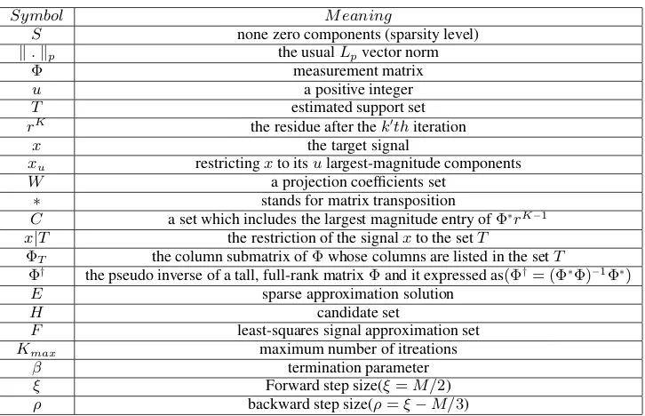
Reconstruction Rate (500 Realizations): M=128, N=256
[image:4.595.325.536.402.578.2]E−OMP OMP ROMP
Fig. 1: Reconstruction results over sparsity for uniform sparse signals employing Gaussian observation matrices.
5 10 15 20 25 30 35 40 45 50 55 0
0.5 1 1.5 2 2.5 3 3.5 4
Signal Sparsity Level
Average normalized mean squared error
Reconstruction Rate (500 Realizations): M=128, N=256
[image:5.595.327.539.69.467.2]E−OMP OMP ROMP
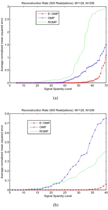
Fig. 2: Reconstruction results over sparsity for Gaussian sparse vectors using Gaussian observation matrices.
5 10 15 20 25 30 35 40
0 0.1 0.2 0.3 0.4 0.5 0.6 0.7 0.8
Signal Sparsity Level
Average normalized mean squared error
Reconstruction Rate (500 Realizations): M=128, N=256
E−OMP OMP ROMP
Fig. 3: Reconstruction results over sparsity for sparse binary signals using Gaussian observation matrices.
that of ROMP is only slightly better. ROMP provides lower error than OMP, however it is still worse than E-OMP, where OMP and ROMP start to fail whenS >6and whenS≥22, respectively and E-OMP fails only whenS >52.
The second set of simulations employ Gaussian sparse vectors, whose nonzero entries were drawn from the standard Gaussian distribution. The results of these simulations forS from 5 to 55 are depicted in Fig. 2.
Fig. 2 depicts the ANMSE rates for this test. In this scenario, E-OMP provides clearly better reconstruction than ROMP and OMP. E-OMP provides lower ANMSE rate than all the other algorithms, where OMP and ROMP start to fail whenS ≥15and
whenS > 45respectively and E-OMP method fails only when
S >47. ROMP yields the worst ANMSE, as a consequence of the
almost complete failure of a non-exact reconstruction.
50 60 70 80 90 100 110 120 130
0 0.1 0.2 0.3 0.4 0.5 0.6 0.7
M
Average normalized mean squared error
Reconstruction Rate (500 Realizations): S=20, N=256
E−OMP OMP ROMP
(a)
50 60 70 80 90 100 110 120 130
0 0.1 0.2 0.3 0.4 0.5 0.6 0.7
M
Average normalized mean squared error
Reconstruction Rate (500 Realizations): S=20, N=256
E−OMP OMP ROMP
(b)
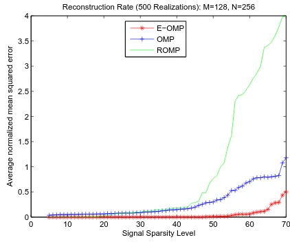
Fig. 4: (a) Reconstruction results over observation lengths for binary sparse signals where S = 20 using a single Gaussian observation matrix for each M., (b)Reconstruction results over observation lengths for binary sparse signals where S = 20 using a Bernoulli distribution matrix for each M.
Next set of simulations employ sparse binary vectors, where the nonzero coefficients were selected as 1. The results are shown in Fig. 3. E-OMP achieve overwhelming success over ROMP and OMP methods in this case, where OMP and ROMP start to fail whenS ≥12and whenS >13respectively and E-OPM method fails only whenS >35.
The success of E-OMP is related to its way to selects the columns of
[image:5.595.64.275.69.245.2] [image:5.595.64.275.307.483.2]0 10 20 30 40 50 60 70 0
0.5 1 1.5 2 2.5 3
Signal Sparsity Level
Average normalized mean squared error
Reconstruction Rate (500 Realizations): M=128, N=256
E−OMP OMP ROMP
(a)
5 10 15 20 25 30 35 40
0 0.1 0.2 0.3 0.4 0.5 0.6 0.7 0.8
Signal Sparsity Level
Average normalized mean squared error
Reconstruction Rate (500 Realizations): M=128, N=256
E−OMP OMP ROMP
(b)
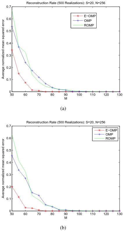
Fig. 5: (a) ANMSE for reconstruction of uniform sparse signals from noisy observations using Gaussian observation matrices., (b)ANMSE for reconstruction of binary sparse signals from noisy observations using Gaussian observation matrices.
5.2 Performance over different observation lengths
Another interesting test case is the reconstruction ability when the observation length,M, changes Fig. 4a depicts the reconstruction performance over M for binary sparse signals whereS = 20
and M is changed from 50 to 130 with step size 5 to observe the variation of the average reconstruction error. For each M value, a single Gaussian observation matrix is employed to obtain observations from all signals. In this test E-OMP clearly provide lower ANMSE than the others methods.
In order to question the choice of the observation matrix, the last scenario is repeated with observation matrices drawn from the Bernoulli distribution. The ANMSE for this test are illustrated in Fig. 4b. Comparing Fig. 4b with Fig.4a, the ANMSE values
remain quite unaltered for E-OMP and ROMP, while that for OMP decreases.
5.3 Reconstruction from noisy observations
Now, reconstruction of sparse signals is simulated from noisy observationsy = Φx+nwhich are obtained by contamination of white Gaussian noise componentn(n= 10−4). The simulation is repeated for 500 binary and 500 uniform sparse signals, where N = 256 and M = 128. The sparsity levels are changed from 5 to 50 and from 5 to 70 with step size 1 for the binary and uniform sparse signals, respectively. The observation matrix Φ drawn from the Gaussian distribution. Fig.5a and Fig.5b depicts the reconstruction error for the noisy binary and uniform sparse signals. In this test E-OMP clearly produces less error than ROPM and OMP.
6. CONCLUSION
In this paper, we have proposed a novel CS reconstruction approach, Enhanced Orthogonal Matching Pursuit (E-OMP), which falling into the category of TST algorithms. By solving the least-square problem instead of using the absolute value of inner product, E-OMP increase the probability to select the correct columns from Φ and therefore, it can give much better approximation performance than all the other tested OMP type algorithms. In addition to, E-OMP uses a simple backtracking step to detect the previous chosen columns reliability and then remove the unreliable columns at each time. In the provided experiments, E-OMP, with some modest settings,performs better reconstruction for uniform and Gaussian sparse signals. It also shows robust performance under presence of noise. E-OMP achieve overwhelming success over ROMP and OMP methods for the sparse binary signals. To conclude, the demonstrated reconstruction performance of E-OMP indicates that it is a promising approach, that is capable of reducing the reconstruction errors significantly.
7. REFERENCES
[1] D. L. Donoho. Compressed sensing. IEEE Trans. Inform. Theory, 52(4):1289–1306, Apr. 2006.
[2] Walid Osamy, Ahmed Salim, and Ahmed Aziz. Efficient compressive sensing based technique for routing in wireless sensor networks. INFOCOMP Journal of Computer Science, 12(1):01–09, 2013.
[3] K. Choi and J. Wang. Compressed sensing based cone-beam computed tomography reconstruction with a first-order method.Med. Phys, 37:5113–5125, 2010.
[4] E. J. Candes and T. Tao. Decoding by linear programming. IEEE Trans. Inf. Theor., 51(12):4203–4215, December 2005. [5] J. Romberg and T. Tao. Robust uncertainty principles: Exact signal reconstruction from highly incomplete frequency information.IEEE Trans. Inform. Theory, 52(2):89509, 2006. [6] Emmanuel J. Cand`es, Mark Rudelson, Terence Tao, and Roman Vershynin. Error correction via linear programming. InFOCS, pages 295–308. IEEE Computer Society, 2005. [7] Joel A. Tropp and Stephen J. Wright. Computational methods
for sparse solution of linear inverse problems.Proceedings of the IEEE, 98(6):948–958, 2010.
[image:6.595.66.274.68.471.2][9] J. A. Tropp and A. C. Gilbert. Signal recovery from random measurements via orthogonal matching pursuit. IEEE Trans. Inform. Theory, 53(12):4655–4666, Dec. 2007.
[10] Joel A. Tropp and Deanna Needell. Cosamp: Iterative signal recovery from incomplete and inaccurate samples. CoRR, abs/0803.2392, 2008.
[11] Wei Dai and Olgica Milenkovic. Subspace pursuit for compressive sensing signal reconstruction. IEEE Trans. Inf. Theor., 55(5):2230–2249, May 2009.
[12] Thomas Blumensath and Mike E. Davies. Iterative hard thresholding for compressed sensing. CoRR, abs/0805.0510, 2008.
[13] Deanna Needell and Roman Vershynin. Uniform uncertainty principle and signal recovery via regularized orthogonal matching pursuit. Found. Comput. Math., 9(3):317–334, April 2009.
[14] D. L. Donoho, Y. Tsaig, I. Drori, and J. L. Starck. Sparse solution of underdetermined systems of linear equations by stagewise orthogonal matching pursuit. IEEE Trans. Inf. Theor., 58(2):1094–1121, February 2012.
[15] Arian Maleki and David L. Donoho. Optimally tuned iterative reconstruction algorithms for compressed sensing. CoRR, abs/0909.0777, 2009.
[16] Honglin Huang and Anamitra Makur. An adaptive omp-based compressive sensing reconstruction method for unknown sparsity noisy signals.SampTA, 2011.
[17] V. Cevher and S. Jafarpour. Fast hard thresholding with nesterovs gradient method. in: Neuronal Information Processing Systems, Workshop on Practical Applications of Sparse Modeling, Whistler, Canada, 2010.
[18] Yu Nesterov. Smooth minimization of non-smooth functions. Math. Program., 103(1):127–152, May 2005.