A Diffusion-Augmented Level Set Method with Efficient
Two Step Implementation
Naitik D. Kapadia
M.tech student, RKDF-IST Bhopal, India
Rinku K. Solanki
M.tech student, NRI Bhopal, India
Bhagwan S. Sharma
Assistant Professor, RKDF-IST Bhopal, India
ABSTRACT
The level set method was devised by Osher and Sethian [2] in as a simple and versatile method for computing and analyzing the motion of an interface Γ in two or three dimensions. Γ bounds a region Ω. The goal is to compute and analyze the subsequent motion of Γ under a velocity field v [1]. This velocity can depend on position, time, the geometry of the interface and the external physics. The interface is captured for later time as the zero level set of a smooth function ϕ(x, t), i.e., Γ (t) = {x|ϕ(x, t) = 0}. ϕis positive inside Ω, negative outside Ω and is zero on Γ (t) [1]. This paper presents a reaction-diffusion method used to describe a physico-chemical phenomenon that comprises two elements, namely chemical reactions and diffusion for implicit active contours[21][37][39][40], which is completely free of the costly re-initialization procedure in level set evolution (LSE). A diffusion term is introduced into LSE, resulting in a diffusion-augmented level set method with efficient two step implementation. First we iteratively solve the diffusion term and then iteratively solve the level set equation. By solving equation in two steps we can stabilize the level set function without re-initialization. This is also called two step splitting method for image segmentation.
General Terms
Image segmentation, two step splitting method, partial differential equation, active contour
Keywords
Level set method, image segmentation, diffusion; level set evolution, re-initialization, signed distance function
1.
INTRODUCTION
Level set methods have seen tremendously applications in many areas over the past decade [13]. This has been made possible by the exibility of the level set formulation in dealing with dynamic evolutions and topological changes of curves and surfaces, and by the mathematical theory and numerical tools developed in studying these methods[15][18][23]. The level set methods (LSM) can be categorized into partial differential equation (PDE) based ones and variational ones. Level set method was first introduced by Osher and Sethian, and has become a more and more popular theoretical and numerical framework within image processing, fluid mechanics, graphics, computer vision, etc.[2] The level set method is basically used for tracking moving fronts [1-2] by considering the front as the zero level set of an embedded function, called the level set function. In image processing, it is used for propagating curves in 2D or surfaces in 3D. The applications of the level set method cover most fields in image processing, such as noise removal, image inpainting, image
International Journal of Computer Applications (0975 – 8887) Volume 70– No.23, May 2013
2.
BACKGROUND AND RELATED
WORKS
The original idea behind the level set method was a simple one. Given an interface Γ in Rn
of codimension one, bounding a open region Ω [1], we wish to analyze and compute its subsequent motion under a velocity field 𝑣 . This velocity can depend on position, time, the geometry of the interface e.g. its normal or its mean curvature and the external physics. The idea, as devised in 1987 by S. Osher and J.A. Sethian [2] is merely to define a smooth function ϕ(x, t), that represents the interface as the set where ϕ(x, t) = 0. Here x = x (x1. . . xn) 𝜖
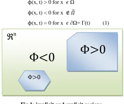
Rn. The level set function ϕ has the following properties ϕ(x, t) > 0 for x 𝜖 Ω
ϕ(x, t) < 0 for x ∉ 𝛺
[image:2.595.68.268.218.385.2]ϕ(x, t) = 0 for x 𝜖 ∂Ω= Γ(t) (1)
Fig 1: implicit and explicit regions
Hence we can identify the interface by locating the set for which Γ(t) for which ϕvanishes. These phenomena can be useful for numerical computation, primarily for topological changes such as breaking and merging [1][2][3]. The motion is analyzed by convecting the ϕ values (levels) with the velocity field𝑣 . This elementary equation is
ddtφ + 𝑣 . 𝛻𝜑 = 0.
(2)
Here 𝑣 is the desired velocity on the interface, and is arbitrary elsewhere. Actually, only the normal component of v is needed: VN = 𝑣 ·𝛻𝜑 , so (1) becomes
ddtφ + VN. 𝛻𝜑 = 0.
(3)
Since F is defined as the speed in the outward normal direction, then 𝑥 · n = F, where n =Δ𝜑Δ𝜑 . This yields an
evolution equation for 𝜑:
ddtφ + F. 𝛻𝜑 = 0. (4) This equation is defined by the authors “osher and sethian”[2]. Using this equation we can find the topological changes using iteration methods. One disadvantage of this level set method is that level set function (LSF) becomes to flat or too steep near the zero level set, causing numerical errors [15][23]. This problem can be solved by re-initializing the level set function and repeat the same procesedure until find the desired level set.
2.1 Re-initialization:
Using re-initialization method we can find topological changes in the image like merging and splitting. a procedure called re-initialization is periodically employed to reshape it to be an SDF [2][8][41]. This method is used extensively with
level set method for stable numerical solution. The standard initialization method is to solve the following re-initialization equation,
φt + Sign(φ0 )(1-|∇φ|) = 0 (5)
Where φ0 is the function to be re-initialized, and sign(φ) is the
sign function. If φ0 is not smooth or is too steeper at one side
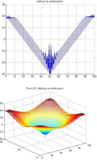
of the interface than the other, the resulting zero level set function may be incorrect from that of the original function. If signed distance function is far away from the level set function then it becomes difficult to re-initialize the level set function to be signed distance function [9]. In practice, the evolving level set function can deviate greatly from its value as signed distance in a small number of iteration steps, especially when the time step is not chosen small enough. Re-initialization has been extensively used as a numerical remedy for maintaining stable curve evolution and having desirable results. The re-initialization process can be quite complicated, expensive and have subtle side effects. Most of the level set methods are fight with their own problems, such as when and how to re-initialize the level set function to a signed distance function.
2.2 Signed distance function:
As to get stable and accurate evolution of topological changes we are initializing the level set function as signed distance function. Osher and Sethian proposed to initialize the LSF as φ(x) =1±dist2
(x), where dist(⋅) is a distance function and “±” denotes the signs inside and outside the contour [9]. Later, Mulder et al.initialized the LSF as φ(x)=±dist(x), which is an SDF that can result in accurate numerical solutions.re-initialization methods do not directly compute the SDF since the solution of |∇φ|=1 is itself an SDF [28]. In, the following re-initialization equation was proposed
φt + S(φ0 )(|∇φ| −1) = 0 (6)
Where S(φ0 )≜ φ
φ2+ ∇φ 2.(∆x)2 , φ0 is the initial LSF and Δx is
the spatial step. Unfortunately, if the initial LSF φ0 deviates
much from an SDF, Eq. will fail to yield a desirable final SDF.
As re-initialization has many drawbacks such as the expensive computational cost, blocking the emerging of new contours, failures when the LSF deviates much from an SDF, and inconsistency between theory and implementation. Solution to this problem is proposed to regularize the variational LSF to eliminate the re-initialization procedure. Li proposed the distance regularized level set evolution (DRLSE) method for accurate evolution of LSF [41]. Li et al. proposed a signed distance penalizing energy functional:
P(φ) = (|∇φ| − 1)Ω 2 𝑑𝑥 (7)
This equation measures the closeness between an LSF φ and an SDF in the domain Ω⊂Rn
.Although DRLSE methods have many advantages over re-initialization methods, such as higher efficiency and easier implementation, they still have
Table 1: Comparison of different level set method
the following drawbacks as limited application to PDE-based LSMs, limited anti-leakage capability for weak boundaries, and sensitivity to noise. By adding the diffusion term into level set method equation and evaluate it in two steps we can get better accuracy and stability in image segmentation and it becomes free from costly re-initialization procedure.
ℜ
nΦ<0
Φ>0
3.
REACTION-DIFFUSION SYSTEM ON
MOVING SURFACES
The term reaction-diffusion system is basically related to physico-chemical phenomenon that comprises two elements, namely chemical reactions and diffusion [16][21]. A chemical reaction system consists of N species (x1. . . xn) (e.g.
molecules) together with M reaction channels, (r1. . . rm). Each
reaction channel defines the stoichiometry of a reaction
rm : ∝𝑖 im Xi
𝑘𝑚
𝛽𝑗 jm Xj (8)
This describes the idea that whenever the species i come together with molar concentrations ∝i, they are interconverted
to the species j with molar concentrations 𝛽j with a specific
reaction rate km. Using the law of mass action , one can derive
a system
𝑑𝑐𝑑𝑡 = k𝑀
1 m (𝛽im - ∝im ) (9)
or in matrix notation
𝑑𝑐𝑑𝑡 = MS . r(t) (10)
Where MS is the stoichiometric matrix and r the rate vector
describing the speed of each reaction.
The second phenomenon, diffusion, refers to the process of thermal motion of molecules [38][39][40]. It is the process by which for example warm and cold water intermingles until the water has a uniform temperature (at thermal equilibrium) or by which a fragrant smell spreads in a room. The general macroscopic diffusion equation for species i = 1, 2,….N is
𝑑𝑐𝑑𝑡= ∇.(Di∇ci ) (11)
where Di denotes the diffusion tensor of species i, a matrix that defines how well the molecule i diffuses into the different spatial directions.
Combining equations and , we get the so called reaction-diffusion equation. The equations for a reaction-reaction-diffusion system on a surface Γ⊂ Ω ⊆ R3
are then
𝑑𝑐𝑑𝑡= Ri(C) + Di∆Γci i = 1,2……N;
Since the zero level is used to represent the object contour, we only need to consider the zero level set of the LSF. We can use a function with different phase fields as the LSF. Motivated by the phase transition theory, by adding a diffusion term into the conventional LSE equation. Such an introduction of diffusion to LSE will make LSE stable without re-initialization. By adding a diffusion term “εΔφ” into the LSE equation, we have the following RD equation for LSM:
φt = εΔφ -
1
ε L(φ), x ∈ Ω ⊂ R
n
4.
TWO STEP DIFFUSION BASED LSM
A Two step algorithm to implement Diffusion has been proposed in to generate the curvature-dependent motion. In the reaction function is first forced to generate a binary function with values 0 and 1, and then the diffusion function is applied to the binary function to generate curvature- dependent motion. Different from, where the diffusion function is used to generate curvature-dependent motion, in our proposed LSM, the LSE is driven by the reaction function, i.e., the LSE equation. Therefore, we propose to use the diffusion function to regularize the LSF generated by the reaction function. To this end, we propose the following two step method to solve the equation.
Step 1: Solve the reaction term till some time Tr to obtain the intermediate solution, denoted by φn+1/2 =φn;
Step 2: Solve the diffusion term φt =εΔφ, φ(x,t=0) = φn+1/2 till some time Td , and then the final level set is φn+1
=φ(x,Td).
4.1 PROPOSED ALGORITHM:
1. Read image
2. Apply Gaussian kernel for smoothing SR
NO .
TITTLE Proposed Method
1 An Efficient Algorithm for Level Set Method Preserving Distance Function
Fast algorithm to preserve distance functions in level set methods. algorithm is inspired by recent efficient ℓ1optimization techniques
2 Re-initialization Free Level Set Evolution via Reaction Diffusion
This paper presents a novel reaction diffusion (RD) method for implicit active contours, which is completely free of the costly re-initialization procedure in level set evolution (LSE). A diffusion term is introduced into LSE, resulting in a RD-LSE equation.
3 Distance Regularized Level Set Evolution and Its Application to Image Segmentation
The DRLSE defined with a potential function such that the derived LSE has a unique forward-and-backward (FAB) diffusion effect, which is able to maintain a desired shape of the LSF, particularly a signed distance profile near the zero level set. 4 A Level Set Method for
Image Segmentation in the Presence of Intensity Inhomogeneities With Application to MRI
This paper proposes a novel region-based method for image segmentation, which is able to deal with intensity in homogeneities in the segmentation.
5 Modified Gradient Search for Level Set Based Image Segmentation
Active contours, gradient methods: (1) resilient propagation (Rprop) (2) using a momentum term image segmentation, level set method, machine learning, optimization, variational problems. SR
NO .
TITTLE Proposed Method
1 An Efficient Algorithm for Level Set Method Preserving Distance Function
Fast algorithm to preserve distance functions in level set methods. algorithm is inspired by recent efficient ℓ1optimization techniques
2 Re-initialization Free Level Set Evolution via Reaction Diffusion
This paper presents a novel reaction diffusion (RD) method for implicit active contours, which is completely free of the costly re-initialization procedure in level set evolution (LSE). A diffusion term is introduced into LSE, resulting in a RD-LSE equation.
3 Distance Regularized Level Set Evolution and Its Application to Image Segmentation
The DRLSE defined with a potential function such that the derived LSE has a unique forward-and-backward (FAB) diffusion effect, which is able to maintain a desired shape of the LSF, particularly a signed distance profile near the zero level set. 4 A Level Set Method for
Image Segmentation in the Presence of Intensity Inhomogeneities With Application to MRI
This paper proposes a novel region-based method for image segmentation, which is able to deal with intensity in homogeneities in the segmentation.
5 Modified Gradient Search for Level Set Based Image Segmentation
International Journal of Computer Applications (0975 – 8887) Volume 70– No.23, May 2013
3. Implementation of Dirac function δ(x)
4. Selection of Time Step value
5. Implementation of penalizing energy term P(\phi) For implementation of penalizing) energy term P(\phi) Set following parameter
u0: level set function to be updated
g: edge indicator function
lambda: coefficient of the weighted length term L(\phi)
mu: coefficient of the internal (penalizing) energy term P(\phi)
alf: coefficient of the weighted area term A(\phi), choose smaller alf
epsilon: the papramater in the definition of smooth Dirac function, default value 1.5
delt: time step of iteration, see the paper for the selection of time step and mu
numIter: number of iterations.
6. Define initial level set function The initial LSF
Φ0(x1,x2) = x1 − 50 2 + (𝑥2 − 50)2 - 30
7. Start level set evolution
8. Optimization of results (final contour detection.)
5. EXPERIMENTAL RESULTS
Fig 2: (a) Testing image. red circle represents the initial contour and Middle slices of level set function during LSE. (b) The final LSFs .The initial LSF is Φ0(x1, x2) =
𝐱𝟏 − 𝟓𝟎 𝟐 + (𝒙𝟐 − 𝟓𝟎)𝟐 - 30. Δt1=Δt2=0.1, Δx1=Δx2=1.
The number of iterations is 100.
Fig 3: (a) Testing image. (b) The final LSFs.image size = 225 x 225 , type: bmp ,Time step(∆𝑻)= 1, Mu (𝝁) =0.2/∆𝑻 , Lambda (𝜸)= 5, Alpha (∝)= -0.3, Epsilon (∈)=1.5, Sigma
(𝝈)= 0.8, iteration = 1500, segment time= 2.03.04 second
Fig 4: (a) Testing image. (b) The final LSFs. Image size = 127 x 96, type: bmp, Time step (∆𝑻) = 1, Mu (𝝁) =0.2/∆𝑻 , Lamda (𝜸)= 5, Alpha (∝)= -0.3, Epsilon (∈)=1.5, Sigma
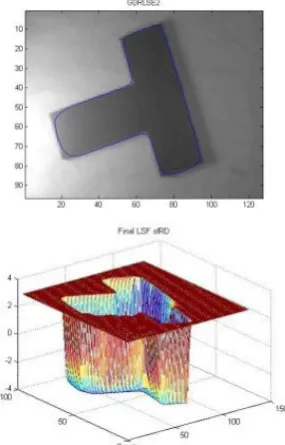
[image:4.595.316.538.75.406.2] [image:4.595.72.255.417.718.2] [image:4.595.360.503.477.700.2]Fig 5: Two step diffusion based LSM method (a) middle slices of the LSFs in iterations (b) the final LSFs. We set
Δt1=Δt2=0.1.
Fig 6: DRLSE method (a) middle slices of the LSFs in iterations (b) the final LSFs. We set Δt1=Δt2=0.1.
Table 2: Comparison of experimental results of Diffusion based LSM and DRLSE method.
6.
CONCLUSION
The Two step diffusion based LSM is general, which can be applied to the PDE-based level set methods and variational ones. Second, method has much better performance on weak boundary anti-leakage. Third, the implementation of the method is very simple and it does not need the upwind scheme at all. Fourth, this method is robust to noise. The experiments on synthetic and real images demonstrated the promising performance of our approach.
7.
ACKNOWLEDGMENTS
Thanking to Ass. Prof. Bhagwan S. Sharma, for his valuable knowledge and support and guiding us to the right path.
8.
REFERENCES
[1] M. Kass, A. Witkin, and D.Terzopoulos, “Snakes: Active
contour models,” Int. J. Comput. Vis., vol.1, pp. 321– 331,1987.
[2] S. Osher and J. Sethian, “Fronts propagating with
curvature dependent speed: Algorithms based on Hamilton-Jacobi formulations,” J. Comp. Phys., vol. 79, pp. 12-49, 1988.
[3] V. Caselles, F. Catte, T. Coll, and F. Dibos, “A
geometric model for active contours in image processing,” Numer. Math., vol. 66, pp. 1-31, 1993
[4] R. Malladi, J. Sethian, and B. Vemuri, “Shape Modeling
with Front Propagation: A Level Set Approach,” IEEE Trans. Pattern Analysis and Machine Intelligence, vol. 27, no. 5, pp. 793–800, 1995.
[5] V. Caselles, R. Kimmel, and G. Sapiro, “Geodesic
Active Contours,” Int. J. Comput. Vis., vol. 22, no. 1 pp. 61–79,1997.
[6] H. Zhao, T. Chan, B. Merriman, and S. Osher, “A Variational Level Set Approach to Multiphase Motion,” J. Comp. Phys., vol. 127, pp. 179-195, 1996.
[7] D. Peng, B. Merriman, S. Osher, H. Zhao, and M. Kang, “A PDE-Based Fast Local Level Set Method,” J. Comp. Phys., vol. 155, pp. 410-438, 1999.
[8] C. Li, C. Xu, C. Gui, and M. D. Fox, “Level set
evolution without re-initialization: A new variational formulation,”Proc. IEEE Conf. Computer Vision and Pattern Recognition, vol. 1, pp. 430–436, 2005.
[9] S. Osher and R. Fedkiw, Level Set Methods and Dynamic Implicit Surfaces, Springer-Verlag, New York, 2002.
∆𝑇 Mu
(𝜇) (𝛾) (∝) (∈) (𝜎) time
DIFFU-LSM
0.1 0.2/∆𝑇 5 -0.3 1.5 0.8 4.8
[image:5.595.88.256.71.347.2] [image:5.595.310.549.84.160.2] [image:5.595.74.274.398.727.2]International Journal of Computer Applications (0975 – 8887) Volume 70– No.23, May 2013
[10] B. Merriman, J. Bence, and S. Osher, “Motion of
Multiple Junctions: A Level Set Approach,” J. Comp. Phys., vol. 112, pp. 334-363, 1994
[11] K. Zhang, L. Zhang, H. Song and W. Zhou, “Active contours with selective local or global segmentation: a new formulation and level set method,” Image and Vision Computing, vol. 28, issue 4, pp. 668-676, April 2010.
[12] M. Sussman, P. Smereka, S. Osher, “A Level Set
Approach for Computing Solutions to Incompressible Two-Phase Flow,” J. Comp. Phys., vol. 114, pp. 146-159, 1994.
[13] R. Tsai, and S. Osher, “Level Set Methods and Their
Applications in Image Science,” COMM.MATH.SCI., vol.1, no. 4, pp. 623–656, 2003.
[14] T. Chan and L. Vese, “Active contours without edges,”
IEEE Trans.Image Process, vol. 10, no. 2, pp. 266–277, Feb. 2001.
[15] G. Aubert and P. Kornprobst, Mathematical problems in image processing, New York: Springer-Verlag, 2000
[16] J. Rubinstein, P. Sternberg, and J. Keller, “Fast reaction,
slow diffusion, and curve shortening,” SIAM J.APPL.MATH, Vol. 49, No. 1, pp. 116-133, Feb. 1989.
[17] J. Xu, H. Zhao, “An Eulerian Formulation for Solving
Partial Differential Equations Along a Moving Interface,” J. Sci. Comp., vol. 19, pp. 573-594, 2003.
[18] J. Strikwerda, Finite difference schemes and partial differential equations, Wadsworth & Brooks/Cole Advanced Books & Software, Pacific grove, California, 1989.
[19] S. Allen and J. Cahn, “A Microscopic Theory for
Antiphase Boundary Motion and Its Application to Antiphase Domain Coarsening,” Acta Metallurgica., vol. 27, pp. 1085-1095, 1979.
[20] S. Baldo, “Minimal Interface Criterion for Phase
Transitions in Mixtures of Cahn-Hilliard Fluids,” Annals Inst. Henri Poincare., vol. 7, pp. 67-90, 1990.
[21] G. Barles, L. Bronsard, and P. Souganidis, “Front Propagation for Reaction-Diffusion Equations of Bistable Type,”Annals Inst. Henri Poincare., vol. 9, pp. 479-496, 1992.
[22] I. Fonseca and L. Tartar, “The Gradient Theory of Phase
Transitions for Systems with Two Potential Wells,” Proc. Royal Soc. Edinburgh., vol. 111A, no. 11, pp. 89-102, 1989.
[23] http://www.engr.uconn.edu/~cmli/
[24] C. Li, C. Kao, J. Gore, and Z. Ding, “Implicit Active
Contours Driven by Local Binary Fitting Energy,” Proc. IEEE Conf. Computer Vision and Pattern Recognition, pp. 1–7, 2007.
[25] L. Modica, “The Gradient Theory of Phase Transitions
and the Minimal Interface Criterion,” Arch. Rational Mech. Anal., vol. 98, pp. 123-142, 1987.
[26] X. Xie, “Active Contouring Based on Gradient Vector
Interaction and Constrained Level Set Diffusion,” IEEE Trans. Image Processing, vol. 19, no. 1, pp. 154-164, Jan. 2010.
[27] D. Chopp, “Computing Minimal Surface via Level Set
Curvature Flow,” J.Comput.Phys., vol. 106, pp. 77-91, 1993.
[28] W. Mulder, S. Osher and J. Sethian, “Computing
Interface Motion in Compressible Gas Dynamics,” J.Compt. Phys., vol. 100, pp. 209-228, 1992.
[29] G. Russo and P. Smereka, “A Remark on Computing
Distance Functions,” J.Comput. Phys., vol. 163, pp. 51-67, 2000.
[30] M. Sussman and E. Fatemi, “An Efficient
Interface-Preserving Level Set Redistancing Algorithm and Its Application to Interfacial Incompressible Fluid Flow,” SIAM J.Sci. Comput., vol. 20, pp. 1165-1191, 1999.
[31] J. Gomes and O. Faugeras, “Reconciling distance
functions and Level Sets,” J.Visiual Communic. And Imag. Representation, vol. 11, pp. 209-223, 2000.
[32] L. Vese and T. Chan, “A multiphase level set framework
for image segmentation using the Mumford-Shah model,” Int. J. Comput. Vis., vol. 50, pp. 271-293, 2002.
[33] S. Ruuth, “A diffusion-generated approach to multiphase
motion,” J.Comput. Phys., vol. 145, pp. 166-192, 1998.
[34] ]S. Ruuth, B. Merriman, “Convolution generated motion
and generalized huygens’s principles for interface motion,”
[35] B. Merriman and S. Ruuth, “Diffusion generated motion
of curves on surfaces,” J.Comput. Phys., vol. 225, pp.2267-2282, 2007.
[36] S. Ruuth, “Efficient algorithm for diffusion-generated
motion by mean curvature,” J.Comput. Phys., vol. 144, pp.603-625, 1998.
[37] S. Zhu and D. Mumford, “Prior Learning and Gibbs
Reaction-Diffusion,” IEEE Trans. Pattern Analysis and Machine Intelligence, vol. 19, no. 11, pp. 1236–1250, 1997.
[38] G. Turk, “Generating Textures on Arbitrary Surfaces
Using Reaction-Diffusion,” Computer Graphics, vol. 25, no. 4, 1991.
[39] A. Witkin, and M. Kass, “Reaction-diffusion textures,”
ACM SIGGRAPH, 1991.
[40] A. Sanderson, M. Kirby, C. Johnson, and L. Yang, “Advanced Reaction-Diffusion Models for Texture Synthesis,” Journal of Graphics Tools, vol. 11, no. 3, pp. 47-71, 2006.
[41] C. Li, C. Xu, C. Gui, and M. D. Fox, “Distance