Munich Personal RePEc Archive
Financial Development and Instability:
the Role of the Labour Share
ORGIAZZI, Elsa
GREQAM
12 October 2007
Online at
https://mpra.ub.uni-muenchen.de/6304/
Financial Development and Instability:
the Role of the Labour Share
∗Elsa ORGIAZZI†
Université de la Méditerranée
GREQAM
October 15, 2007
Abstract
This paper examines the role of the labour share in creating instability in a small open
econ-omy. We assume that financial markets are imperfect so that entrepreneurs are credit constrained,
and that this constraint is tighter for low levels of financial development. Aghion, Bacchetta and
Banerjee (2004) have shown that as the degree of financial development increases, output rises
but instability appears for intermediate levels of financial development. Crucially, they assume
that labour is paid before production takes place, and hence crises are solely due to the increased
cost of debt repayment as firms accumulate capital. We show that under the more reasonable
assumption that wages are paid at the end of the period, changes in the labour share also play a
role in eroding profitability. Our analysis also predicts that financial crises are associated with
substantial movements in the sharing of value added between capital and labour.
Keywords: Financial liberalization, Volatility, Labour share, Credit constraint
JEL classification numbers: E32, F40, E25
∗I am grateful to Cecilia García-Peñalosa for her continuous feedback, useful comments and suggestions. I also thank
Patrick Pintus and workshop participants at GREQAM.
†
1
Introduction
The financial liberalization which took place at the end of the seventies for industrial countries, and in the nineties for developing ones, has been justified by many arguments. Financial liberalization is sup-posed to increase market efficiency by creating possibilities for diversification and leading to a better allocation of investment (see Fama (1970)). Opening up financial markets is expected to increase the productive capital stock in a country by facilitating borrowing for entrepreneurs. As a result, the grow-ing capital flows that we have observed are supposed to have created new investment possibilities and promoted growth. Moreover the diversification resulting from the deregulation of financial markets should have reduced volatility. This last argument, however, does not seem to be supported by empir-ical evidence. First, there are no empirempir-ical cross-country studies showing that financial liberalization stabilizes an economy, whereas there is some evidence of a positive correlation between financial integration and volatility; see Kose et al. (2002). Second, the experience of Argentina, Mexico, Rus-sia, and the South-East Asian countries seems to indicate that periods of financial liberalization have coincided with financial crises in emerging countries.
The literature has found several explanations of financial crises, from herd behavior to corruption, trade imbalances or excessive external claims. Here we follow Aghion et al. (2004) who show that opening up financial markets leads to endogenous volatility when firms face credit constraints. Fi-nancial market imperfections are central in the analysis of procyclicity of capital flows, as shown by Kaminsky et al. (2004), and are hence a possible cause of crises. Moreover, since firms in emerging countries are more likely to face credit constraints than those in developed countries, the developing economies are particularly vulnerable.
amount that is proportional to the entrepreneur’s wealth. The ratio of loan to wealth can be seen as measure of the degree of financial market development, as in Aghion et al. (2004).
Our analysis differs from Aghion et al. (2004) in that we emphasize the role of the labour share in generating cycles. Recent empirical evidence has shown that the the labour share varies substantially both across countries and over time.1 Our interest in the role of the labour share is motivated by the work of Diwan (1999). Using data for the last decades of the 20th century, Diwan finds that in most countries the labour share increased before a financial crisis,2and fell by an average of6.12percentage points following the crisis. In many instances, the labour share did not return to its pre-crisis value, indicating that crises tend to be associated with a permanent transfer of income from labour to capital. This evidence raises the question of why is it that the labour share fluctuates together with output.
We make two crucial assumptions. First, as in Aghion et al. (1999) and Aghion et al. (2004), we distinguish between investors and lenders in the sense that not all individuals are capable of becoming entrepreneurs. Second, we assume that output is produced by a CES production function and suppose that labour and capital are complements, in line with existing evidence for low- and middle-income countries; see Duffy and Papageorgiou (2000). Contrary to financial capital3, labour is supposed to
be immobile across countries, and hence the wage rate is equivalent to the real exchange rate. Aghion et al. (2004) make the unusual assumption that wages are paid before production takes place, which implies that a higher labour share does not affect ’profits’ and hence has no impact on the entrepreneurs borrowing capacity. In this paper we make the more standard assumption that the wage bill is paid after production has taken place, which implies that as capital accumulates and the labour share rises, profitability declines. Two main results emerge. First, we show that in this case fluctuations appear for much lower levels of financial development. Second, the elasticity of substitution in production becomes an essential determinant of the dynamics of capital and output, and volatility is greater the stronger the complementarity between capital and labour is.
Section 2 describes the model, the process of wealth accumulation and the role of the labour share. Section 3 obtains the dynamics of capital and the labour share. Section 4 examines why cycles are
1
See, for example, Bentolila and Saint-Paul (2003), Harrison (2002), Bertola (1993), Daudey and Garcia-Peñalosa (2007) and as well Solow (1958) and Kravis (1959).
2
According to Frankel and Rose (1995), the financial crisis is defined as a year in which nominal exchange rate depreci-ates more than 25%
3
more likely to happen when wages are paid at the end of each period, and we then provide some numerical examples. Section 6 concludes.
2
The Model
2.1 Production and Preferences
We consider a small open economy, with a single goodY produced with capital and labour. The economy is populated by two distinct categories of individuals. On the one hand, there areL worker-lenders in the economy, who cannot directly invest in production. They can lend their wealth to domestic entrepreneurs or in the international financial market, and they are employed by the en-trepreneurs. On the other, there areN identical entrepreneurs who can invest directly in production. They employ those who are not entrepreneurs, hence L denotes also the aggregate labour supply. They may also borrow in order to use a capital stock larger than their own wealth. For simplicity we suppose thatN = 1.
We suppose that all entrepreneurs have an identical production function characterized by constant returns to scale. As a result we can define an aggregate production function, which will depend on the aggregate (or average) stock of capital, K, and on labour, L. We suppose that entrepreneurs’ production function is of the constant elasticity of substitution form,
Y =A[K−ρ+L−ρ]−1/ρ, withρ >−1andρ= 0 (1) and that the final good is the numeraire. We also define output per worker as
y=A[1 +k−ρ]−1/ρ, (2)
this parameter is significantly lower than unity, supporting the complementarity between capital and labour in developing countries4. In what follows we will hence suppose that capital and labour are complements, that isρ >0, implyingσ <1.
Labor is assumed to be immobile, inelastic and constant. The labour market is competitive, hence labour is paid its marginal product and there is full employment. Capital is assumed to be internation-ally mobile,5 although we allow only for international flows of financial capital and not for foreign direct investment. Moreover, we assume that capital fully depreciates each period so that the invest-ment of entrepreneurs at timetis equal to the capital stockKt. The international capital market clears
at a gross interest raterwhich is exogenous to our economy and assumed to be lower than total factor productivity in the economy, i.e. r < AWe suppose, however, that financial markets are imperfect and that entrepreneurs are credit constrained. Entrepreneurs can only borrow up to a fractionµ > 0
of their current wealthWt. This fraction is assumed to be constant and exogenous,6following Aghion
et al. (2004) and Bernanke and Gertler (1989). We can interpret this parameter as the degree of finan-cial liberalization in the economy, with a higher value ofµimplying greater financial liberalization.
As Aghion et al. (2004), we suppose that all agents consume a fixed fraction α of their end of period wealth, where0<α <1, and hence they save a fraction(1−α)of it.
2.2 Factor returns, profits and the labour share
2.2.1 Factor returns
Labour market is perfect hence labour is paid its marginal product:
w≡ ∂Y
∂L =A
1 +k−ρ−
1+ρ
ρ . (3)
Note that since labour is specific to the country, we can interpret the wagewas the exchange rate. The return to capital is :
4
The theoretical foundations for such result have been provided by Miyagiwa and Papageorgiou (2007) in a multi-sectorial model.
5As argues by Rodrik (1998), among others, labour is much less mobile than capital. 6
q ≡ ∂Y
∂K =A(1 +k
ρ)−1+ρρ
. (4)
If the entrepreneurs are unconstrained, the marginal product of capital is equal to the interest rate. However, when the borrowing constraint is binding, entrepreneurs cannot invest as much as as they want and the level of capital stock is lower than the optimal one. Then, the marginal product of capital is greater than the interest rate.
2.2.2 Profits and the labour share
Assuming that wages are paid after production takes place, we can define profits7as output minus the wage bill, that is,
Π≡Y −wL.
Substituting for the wage (3) and for output per worker (2) we obtain profit per worker, denotedπ, which is given by :
π ≡ Π
L =Ak
−ρ1 +k−ρ−1+ρρ
. (5)
We are interested in the role of the labour share. We define it as the ratio of total employee compensation to output and denote it byθwhere
θ≡ wL
Y =
1
1 +k−ρ. (6)
This relationship is important and will be used all along our analysis. It implies that for each capital-labour ratio there is a unique level of the capital-labour share, and vice versa.
Note that per capita output can be expressed as a function of the labour share, namely,
y =Aθ1/ρ. (7)
Forρ >0, a higher labour share is associated with higher level of output per-worker. The reason for this is that, withρ >0, a higher capital-labour ratio results in both a higher labour share and higher
per capita output. Similarly, the marginal products of labour and capital can also be written in terms of labour share,
w=Aθ1+ρρ, (8)
q =A(1−θ)1+ρρ. (9)
Profit per worker can also be defined as a function of the labour share. By definition, profit per worker is the share of value added received by the entrepreneurs after having paid labour costs, that is
π = (1−θ)y(θ) =A(1−θ)θ1/ρ. (10) We can immediately see that the labour share has two opposite effects on profits. First, there is a direct effect as a higher labour share tends to reduce profits for a given level of output; second, a higher labour share is associated with higher output per worker, and hence tends to increase profits.
2.2.3 The effect of capital accumulation on profits and on the labour share
We now examine the effect that capital accumulation has on the labour share and profits. Differenti-ating equation (6) we have
dθ dk =
ρk−(1+ρ)
(1 +k−ρ)2
which is positive ifρ >0and negative forρ <0. Hence, under our assumption that labour and capital arecomplements, the labour shareincreaseswith capital accumulation. Although capital accumula-tion tends to raise capital intensity and hence the capital share, it also reduces the marginal product of capital. When capital and labour are complements, the second effect dominates, hence the capital share falls and the labour share increases.
Consider now the effect of capital accumulation on profits. From equation (5) we can show that8
∂π
∂k >0if and only if k
−ρ > ρ. (11)
8
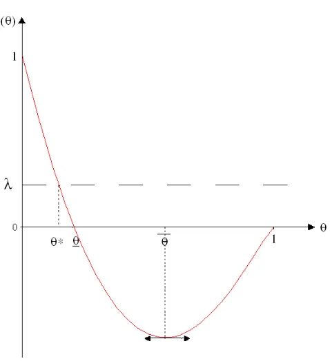
From this condition we can immediately infer that if ρ <0, thendπ/dk >0for allkimplying that in this case profits always increase with capital accumulation. However, for ρ >0, the effect of capital accumulation on profits is non-monotonic. Profits first increase and then decrease, and there exists a threshold level of the capital-labour ratiok≡ρ−1/ρsuch that fork < kthendπ/dk > 0,while for
k > kprofits are decreasing ink.
To understand this note that it is possible to express the threshold as a threshold in terms of the labour share. Indeed,dπ/dk >0if and only ifθ < θ,where
θ≡σ = 1 1 +ρ
A higher capital-labour ratio has two effects on profits. First, it increases output per worker and hence profitability. At the same time, and under our assumption that σ < 1, a higher capital-labour ratio raises the labour share and reduces the capital share. For small values ofk,and hence of the labour share, the output effect dominates; as the capital-labour ratio rises the labour share becomes so high that any further increase inθactually leads to a reduction in profitability.
It is important to note that the behavior of profits in equilibrium differs from that of individual profits. From the point of view of an individual entrepreneur, who takes the wage as given, profits are always increasing in his own stock of capital (see Appendix).
2.3 Capital accumulation
The dynamics of the model are driven by the accumulation of capital by entrepreneurs. In order to obtain the dynamic equation for capital we need to know whether or not entrepreneurs are credit constrained. Define the optimal capital stock, denoted Ku, as the stock that equates the marginal
product of capital to the interest rate, which is given by:
Ku=
A
r
ρ 1+ρ
−1 1/ρ
L≡kuL (12)
An entrepreneur with wealthWtcan investat most(1 +µ)Wt, then
If (1 +µ)Wt is superior toKu, then entrepreneurs are unconstrained and they invest at every
period the optimal level of productive capitalKu. In this case, the capital stock jumps to the levelKu
and there are no dynamics. Given our assumption on savings, the wealth of entrepreneurs is given by
Wt+1= (1−α)rWt. As long as their savings are less thanKuthey will borrow, while once they have
accumulated sufficient wealth to financeKu, they will lend their reminding savings at the market rate
r.
If the maximum level of capital that entrepreneurs can invest is below Ku then they are credit
constrained. They borrow as much as they can, that isµWt. In this case, the capital stock invested at
tis proportional to the wealth of entrepreneurs and given by :
Kt= (1 +µ)Wt (13)
Our assumption on the saving rate together with the binding credit constraint implies that we can write the wealth of the entrepreneurs at timet+ 1as a function of profits and the level of wealth att,
Wt+1 = (1−α)[Πt−rµWt], (14)
where the termrµWtrepresents the debt repayment andΠtare the profits received by an entrepreneur.
3
Dynamic behavior
3.1 Capital accumulation with borrowing constraint
If the borrowing constraint is binding, the capital stock is proportional to wealth (13) which implies that, given the expressions for wealth (14), we can write the dynamic equation for the stock of capital as follows:
Kt+1 = Φ(Kt) = (1 +µ)(1−α)
Πt− rµ
1 +µKt
. (15)
Rewriting (15) in terms of capital per worker, and substituting for profits (5), we obtain the dy-namic equation for the stock of capital per worker9:
kt+1=ϕ(kt) = (1 +µ)(1−α)
Ak−tρ(1 +kt−ρ)−1+ρρ − rµ
1 +µkt
. (16)
Before we examine under which conditions the economy is constrained, we study the properties of the functionϕ(kt). First, note that the function ϕ(kt) takes the value 0 both at kt = 0 and at
kt= λ− ρ 1+ρ −1
1/ρ
> ku, whereλ≡ A(1+rµµ). Secondly, differentiating (16) we obtain :
ϕ′(kt) = (1 +µ)(1−α)
dπ
t
dkt
− rµ
1 +µ
(17)
= (1 +µ)(1−α)A[x(θt)−λ]
where10
x(θt)≡(1−θt) 1+ρ
ρ [1−θt(1 +ρ)]. (18)
Henceϕ′(k
t) > 0if and only if x(θt) > λ. In the appendix we examine the functionx(θ). Since
our assumption that A > r impliesλ < 1, we can show that there exists an unique valueθ∗ such
thatx(θ∗) =λ. Hence there exists a corresponding unique value ofk
tdenotedk∗such thatϕ(kt)is
increasing inktfor allkt< k∗, and decreasing forkt> k∗: the function has a unique maximum atk∗.
Moreover, note thatϕ(kt)is concave at least for values of the capital stock less thank= (1+ρρ)1/ρ.11
The functionϕ(kt)has a unique fixed point, i.e. a steady state denotedk=ktwhich is given by:
k= b−1+ρρ −1
1/ρ
, (19)
where
b≡ 1 +rµ(1−α)
A(1−α)(1 +µ).
.
Note that for an interior steady state to exists, ϕ′(0)has to be greater than 1, which from (17)
requires
A > 1−rµ(1−α)
(1−α)(1 +µ), (20) 10The functionxcan be expressed as a function of capital-labour ratio:x(k) =k−(1+ρ)(k−ρ−ρ)(1 +k−ρ)−1+2ρ
ρ
11See the appendix for an analysis of the second derivative ofϕ(k
that is the total factor productivity has to be sufficiently large.
Note that from (17) and (19), we obtain that the derivative ofϕ(kt)evaluated at the steady statekis
given by :
ϕ′(k) = (1 +µ)(1−α)A ρb1+ρρb1+ρρ −1
−λ
The slope at the steady state may be positive or negative, depending on whetherkis smaller or greater thank∗.
3.2 The effects of financial liberalization
A crucial parameter determining both the dynamics and the type of regime isµ. In this subsection we examine its impact onϕ(kt)and we will consider possible regimes in subsection3.3.
First, differentiating (19) with respect toµ, we can see thatdk/dµ >0provided thatr <1/(1−
α). This condition is satisfied for any realistic value of the saving rate. For example, a large value of
(1−α), say(1−α) = 0.9would requirer to be less than1.11, which would certainly be satisfied for any reasonable configuration. In what follows we will suppose that the restriction is satisfied so that a weaker borrowing constraint raises the stationary value of the capital-labour ratio. As we will see later, this will imply that cycles are more likely to occur at an intermediate stage of financial development than at a stage when the borrowing constraint is tight. Moreover, note that a weaker borrowing constraint raises also the stationary value of output and of the labour share : dy/dµ > 0
anddθ/dµ > 0, with:
θ= 1−b1+ρρ
and
y =A1−b1+ρρ
1/ρ
.
Second, the derivative ofϕ(kt)with respect toµis strictly positive provided thatktis less thanku.
increases withµ.
3.3 Possible regimes
There are two possible regimes: either the economy is always constrained, or the borrowing constraint eventually stops binding. We examine these in turns.
To do that, recall thatk∗denotes the value of the capital stock at which the functionϕ(k
t)reaches
its maximum ϕ(k∗) and thatϕ(k∗) is increasing with µ. This implies that there is a unique value
µu such that for all µ ≥ µu we haveϕ(k∗) ≥ ku. Hence µu defines the lowest level of financial
liberalization which ensures that, at some point in time, entrepreneurs will no longer be constrained. For all µ < µu, entrepreneurs are always constrained unless the initial capital stock is k0 ≥ ku.
Unfortunately, we cannot get the analytical expression of k∗ which prevent us from obtaining an
expression forµu.
Constrained regime:
Ifµ < µuthenϕ(k∗)< ku. In this case the dynamics of the capital stock are given by:
kt+1=
⎧ ⎪ ⎪ ⎨ ⎪ ⎪ ⎩
ϕ(kt)ifkt< ku
kuifkt≥ku
(21)
Note that if the economy starts with an entrepreneurial wealth aboveku, entrepreneurs can finance
the optimal stockku, and the economy will be atkufor ever.
In this regime, there are various possible dynamics paths:
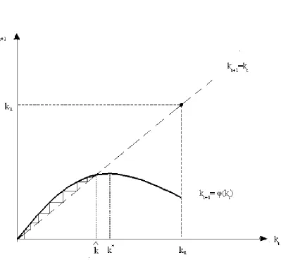
1. Ifk < k∗, the capital stock converges monotonically to the steady state.
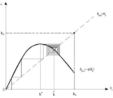
2. Ifk > k ∗, then various scenarios are possible : monotonic convergence, cyclical convergence,
permanent cycles or divergence.
Three possible cases are depicted graphically in figures 1,2and3. Figure1represents the case in which the steady state capital stock is to the left of the maximum of theϕ(kt) schedule, that is
k < k∗. In this case the capital stock increases until it reaches the steady state k. Figures 2and
cycle. Unfortunately, it is not possible to obtain analytical conditions indicating when each of these scenarios would prevail. Hence, in section 5 we will perform numerical simulations to identify under which parameter values volatility appears.
[Figure 1 about here.] [Figure 2 about here.] [Figure 3 about here.]
Unconstrained Regime:
For a level of financial liberalization greater or equal toµu,ϕ(k∗) ≥ku. This means that there
can be a point at which entrepreneurs are not constrained and which allows them to invest as much as they want, that isku. Indeed,kurepresents the maximum amount that entrepreneurs want to invest in
their own technology. Ifku is reached, the economy stays at this level. In this case, the dynamics of
capital stock are described by :
kt+1=
⎧ ⎪ ⎪ ⎨
⎪ ⎪ ⎩
ϕ(kt)ifϕ(kt)< kuandkt< ku
ku otherwise.
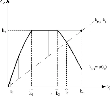
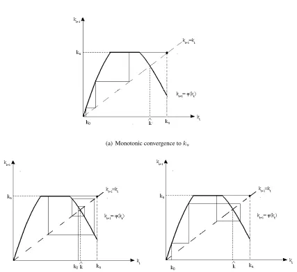
Let us definek˜1 and˜k2 such thatϕ(˜k1) = ϕ(˜k2) = ku with˜k1 < k˜2. Sinceϕ(kt)is concave
anddϕ(kt)/dµ >0for allkt< ku, then˜k1 is decreasing withµwhereask˜2is increasing. Therefore
the higherµis, the greater the range of values ofkfor which entrepreneurs will not be constrained (see figure 4). In the unconstrained regime, the economy will converge toku, either monotonically or
cyclically depending on the value ofµ > µuand the initial level of capital (See in appendix figures
10).12
[Figure 4 about here.]
12
Note that if|ϕ(k)|<1
4
Alternative definition of profits
So far we have assumed that labour is paid at the end of each period, and hence profits are defined as
Πt=Yt−wtL. Aghion et al. (2004) use an alternative assumption. They assume that wages are paid
at thebeginningof each period. This has important consequences for the dynamics of wealth. Under their assumption, total wealth at the beginning of the period is used to finance both wages and new capital, that is
Kt= (1 +µ)Wt−wtL. (22)
This in turn implies that ‘profits’ are equivalent to output, i.e.
Πt=Yt=A[1 +kt−ρ]−1/ρL, (23)
Note that, contrary, to our previous setup, profits are always increasing in the capital stock. The equation driving the accumulation of wealth is now
Wt+1= (1−α)[Yt−rµWt]. (24)
Clearly the negative effect of an increase in entrepreneurs’ wealthWt on next period wealthWt+1
comes solely from the impact of debt repayment. If we compare this expression to that in equation (14), that is
Wt+1= (1−α)[(1−θt)Yt−rµWt], (25)
we can see that when wages are paid at the end of the period there are two effects that tend to reduce future wealth: debt repayment and the fact that, as the capital stock increases, the labour shareθtalso
increases, thus reducing profitability for any given level of output.
The question that arises, then, is whether the assumption on the payment of labour affects the likelihood that cyclical behavior is observed. To address this question we obtain the dynamic equation for capital under the assumption that labour is paid at the beginning of the period.13 From (22) and
13
(24) we find that the dynamics of capital per worker are governed by:
kt+1= (1 +µ)(1−α)
yt− rµ
1 +µwt− rµ
1 +µkt
−wt+1, (26)
which implicitly defineskt+1as a function ofkt, i.e.kt+1=ψ(kt). The dynamic equation for capital
is again non-monotonic inkt.
To examine the dynamics ofkt, we differentiate equation (26) to obtain
dkt+1
dkt
= (1 +µ)(1−α)[dyt
dkt
− rµ
1 +µ− rµ
1 +µ dwt
dkt
]−dwt+1
dkt
. (27)
Noting that
dyt
dkt
= A(1−θt) 1+ρ
ρ , (28) dwt
dkt
= A(1 +ρ)θt(1−θt) 1+ρ
ρ , (29) dwt+1
dkt
= dwt+1
dkt+1
dkt+1
dkt
=A(1 +ρ)(1−θt+1)
1+ρ ρ θ
t+1
dkt+1
dkt
, (30)
and substituting for these expressions into (27) we have
dkt+1
dkt
= (1 +µ)(1−α)A 1 +A(1 +ρ)(1−θt+1)
1+ρ ρ θt+1
(1−θt) 1+ρ
ρ (1−λA(1 +ρ)θ t)−λ
. (31) As before, we concentrate in the case in whichλ <1. In this case, theψ(kt)schedule is increasing
if and only if
z(θt)> λ,
where
z(θt)≡(1−θt) 1+ρ
ρ (1−λA(1 +ρ)θt) (32)
It is possible to compare the dynamic schedules obtained under the two assumptions for profits (see appendix) and show that the maximum ofψ(kt), denotedθA∗ is to the right of the maximum of
r <1 + 1
µ, (33)
that is, if thenetinterest rate is less than the inverse ofµfactor. This is a reasonable condition, as will become apparent in our numerical simulations in section 5.3. For instance, if the net interest rate is
0.05, this condition is satisfied forµ <20.
If condition (33) holds, it is then more likely that cyclical behavior takes place when wages are paid at the end than at the beginning of periods. The intuition for this is clear from equations (24) and (25). For Aghion et al. there is a single mechanism that tends to reduce wealth as the capital stock increases : the cost of debt repayment. In this case, wealth -and hence the capital stock- increase as long as profits, which they define as equal to output, increase faster than the cost of repaying the debt,rµWt. In our setup, there is a further force tending to reduce the wealth of entrepreneurs,
namely, the increase in the labour share brought about by a higher capital stock. Since the labour share increases withk, profits grow more slowly than output does. At the same time, the debt burden
rµWtis increasing just as for Aghion et al., implying that the reduction in entrepreneurial wealth will
come about for a lower level of the capital stock than when profits are equal toYt.
5
Numerical examples
5.1 Financial liberalization and cycles
Our analytical results indicate that several patterns of dynamic behavior are possible. In this section we perform numerical simulation to see what type of dynamics prevail for reasonable parameter values. We follow closely the calibrations in Aghion et al. (2004) and set the parameter values as follows:14 total factor productivity A = 3, the gross interest rate r = 1.02, the consumption-to-income ratio
α = 0.7, andρ = 2. This last value corresponds to an elasticity of substitution between capital and labour of1/3.
We start by considering the role of financial liberalization and how it generates cycles, and do so by examining the dynamics of the capital stock for different degrees of financial liberalization, ranging fromµ=1 toµ= 4.5. Aghion at al. (2004) use a value ofµ= 4in their simulations, which
implies that entrepreneurs must have assets equal to one fifth of their total investment, a plausible value. Table 1 gives the steady state capital-labour ratios and per capita income levels for the various values ofµ. As we saw analytically, greater financial liberalization is associated with higher steady state capital and output. However, the economy does not converge to its steady state for eitherµ= 3.5
orµ= 4. Forµ= 3.5, capital and output oscillate on 2-periods cycles, taking alternatively the values
k1= 0.5098andk2 = 0.9140for capital andy1 = 1.3625andy2= 2.0240for output. Note that the
average value of output is1.6932,and thus lower than the steady state value1.8013. [Table 1 about here.]
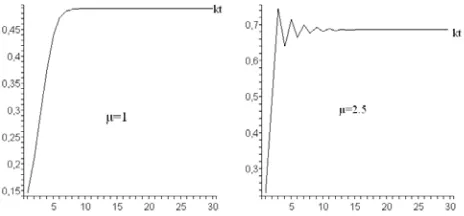
The effect of µ on the dynamic behavior is depicted in figures 5(a) to 5(e). Figure 5(a) considers the case in which µ = 1. There is very limited borrowing and this implies that the steady state capital stock and per capita output will be low. However, the economy is characterized by stability as it converges monotonically to its steady state. As financial markets liberalize, output per capita increases. For µ = 2.5 the economy still converges to its steady state although with oscillations. For µ = 3.5 there is no convergence, but rather the economy oscillates permanently generating a two-period cycle. 4-period oscillations are obtained forµ= 4. These examples indicate that greater financial market liberalization results in greater volatility as long as entrepreneurs are credit constraint. However, above the threshold level of financial liberalizationµu, entrepreneurs will eventually not be
credit constrained and will be able to invest the optimal level of capitalku. For our set of parameter
values,kutakes the value1.0261andµuis equate to4.2. This case is depicted in figure 5(e).
[Figure 5 about here.]
5.2 The role of the elasticity of substitution
We next turn to the role played by the elasticity of substitution between labour and capital. For
ρ > 0, that is, when labour and capital are complements, capital accumulation increases the labour share, which tends to erode profits. Since the labour share is given byθ = 1/(1 +k−ρ), the lower
fluctuations occur. This is exactly what we observe in figures8to13. Following Aghion et al. (2004), we pose µ = 4and allowρ to vary from 0.7 to2, which implies that the elasticity of substitution elasticity varies between0.58and0.33. We can see that as the complementarity between capital and labour increases, cycles appear. A 2-period cycle appears for an elasticity of substitution of0.36.
These figures indicate that the behavior of the labour share, which is in turn determined byρ, plays an important role in creating fluctuations.
[Figure 6 about here.]
5.3 The role of the labour share
Lastly, we provide numerical examples that help us understand the role that the labour share plays in creating volatility through its effect on wealth dynamics. In our benchmark economy in which wages are paid at the end of periods, profits are then given byΠt= (1−θt)Ytand hence wealth dynamics
are driven by the equationWt+1 = (1−α)[(1−θt)Yt−rµWt]. Recall that in Aghion et al., wages
are paid at the beginning of periods, implying that profits are equal to output Πt = Yt and hence
Wt+1= (1−α)[Yt−rµWt].
We setA= 3,r = 1.02,α= 0.7, as above, fix the elasticity of substitution at 1/3 (i.e.ρ= 2)and allow the degree of financial liberalizationµto vary. Table2reports the patterns obtained for different values ofµunder the two scenarios. We can see that in line with our analytical results in section4, the labour share plays an important role in creating cycles. WhenΠt=Yt, the possibilities for borrowing
must be substantial - at leastµ= 9- for the economy to exhibit a two-period cycle. In contrast, when we allow the labour share to affect profitability a much lower value ofµ-namely,µ= 3.5- suffices to generate permanent oscillations.
[Table 2 about here.]
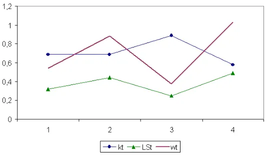
share increases, eroding profitability which in turn reduces borrowing possibilities and triggers the financial crisis. Figures 7(a) and 7(b) depict the behavior of the capital-labour ratio, the labour share, output and wages. As we have argued, wages represent the real exchange rate since labour is immo-bile across countries. We suppose that the economy has initially a low level of financial development,
µ=2.5, and that it is at its steady state. Then, financial market liberalization takes places resulting in a higher borrowing ratio,µ= 4.15
[Figure 7 about here.]
Figure14shows that following financial liberalization the exchange rate appreciates and the labour share increases. One period latter, att=2, the capital stock increases. The rise of the labour share erodes profitability and induces the financial crisis, captured by the fall in the exchange rate att=3. Note that the labour share also falls at this point. Figure15also depicts the dynamics of output, and indicate that the labour share and the exchange rate (wage rate) move together and are countercyclical.
6
Conclusion
A large literature has argued that financial liberalization is beneficial for growth as it results in a better allocation of savings, diversification, and budget austerity policies aimed at attracting funds. Yet the evidence concerning the late 20th century indicates that financial liberalization can also create output volatility in emerging economies; and as Ramey and Ramey (1995) show, higher volatility is associated to lower growth. Our paper has shown how the labour share plays an important role in explaining why liberalizing financial markets create volatility.
Our analysis follows Aghion et al. (2004) and describes a dynamic open economy in which entrepreneurs are credit constrained. Contrary to these authors, profits are defined as output minus the wage bill, and as a result movements in the labour share affect profitability. Since the amount that can be borrowed by entrepreneurs is assumed to be proportional to the entrepreneur’s wealth, this has important implications for the dynamics of the economy. Under the assumption of complementarity between labour and capital, the increase in the capital stock due to financial liberalization increases
15
the labour share and tends to reduce profits. This effect adds to the debt repayment effect analyzed by Aghion et al. (2004), and results in fluctuations for much lower levels of financial development.
7
Appendix
7.1 Capital accumulation and individual profits
In the text we have shown that, in equilibrium, profits are first increasing and then decreasing in the capital stock. However, from the point of view of an individual entrepreneur who takes the wage rate as given, profits are strictly increasing in his own capital stock. To verify this consider the profits of entrepreneur j, defined asΠj = F[Kj, Lj]−wLj. The optimal level of employment can then be
obtained from profit maximization and shown to be proportional to the capital stock:
Lj =
A w ρ 1+ρ −1 1/ρ
Kj.
We can then write profits as
Πj =w
A w ρ 1+ρ −1 1+ρ ρ Kj.
Then∂Πj/ ∂Kj >0as long as the term in square brackets is positive, which forρ >0is the case
if and only ifA > w. Recall thatw=A[1 +k−ρ]−1+ρρ
, which impliesA > wfor allk.
7.2 Concavity of Profits
In order to check whether profits are concave, differentiate (5) to get
d2πt
dk2
t
=−A(1 +ρ)(1 +k −ρ
t )−1/ρ kρt −ρk2tρ+ρkρt
k2
t(1 +kρt)3
,
implying that
d2πt
dk2
t
>0if kt> k≡
1 +ρ
ρ
1/ρ
.
Note that k > k since for ρ > 0, ((1 +ρ)/ρ)1/ρ > ρ−1/ρ. Therefore, if capital is less than the
threshold levelk, then profits are concave. In other words, as long as profits are increasing inkthey will also be concave. Clearly, if profits are concave so is the dynamics equation for capital as
d2kt+1
dk2
t
= (1 +µ)(1−α)d
2π
t
dk2
7.3 Study of the functionx(θ)
Recall that x(θ) = (1−θ)1+ρρ[1−θt(1 +ρ)]. x(θ) takes the value1 at θ = 0 and0 at θ = 1.
Moreover, differentiatingx(θ)we have:
dx(θ)
dθ =−(1 +ρ)(1−θ)
1/ρ1−θ(1 +ρ)
ρ + 1−θ
.
Hencex(θ)is decreasing ifθ < 1+21+ρρ ≡ θand increasing forθ > θ. The functionx(θ)crosses the abscises axe atθ= 1+1ρ ≡θ < θand is convex.
The functionx(θ)is depicted in figure (8). Sinceλ <1, there exists a unique value of the labour shareθ∗such thatx(θ)> λifθ < θ∗andx(θ)< λotherwise.
[Figure 8 about here.]
7.4 The dynamics of the labour share and wages
We turn now to the dynamic behavior of the labour share. Substituting for θ in equation (16), we obtain the dynamics of the labour share which are governed by
θt+1=
1 + 1−θt
θt
[A(1 +µ)(1−α)]−ρ
(1−θt) 1+ρ
ρ −λ
−ρ−1
. (34)
Differentiating
dθt+1
dθt =
θt+1
kt+1
dkt+1
dkt
kt
θt,
which, sinceθt+1/kt+1andkt/θtare both positive, implies that the sign ofdθt+1/dθtis the same as
that ofdkt+1/dkt. Hence
dθt+1
dθt
>0 if and only if θ < θ∗. (35) That is, the labour share has the same behavior as capital. Lastly, recalling that the wage is give by
wt=A
1 +kt−ρ−
1+ρ ρ
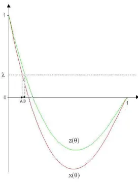
7.5 Comparison of the functionsx(θ)andz(θ)
We have shown that when wages are paid at the end of each period,dkt+1/dkt > 0if and only if
x(θt)> λ, and that this condition turns to bez(θt)> λif wages are paid at the beginning.
Lets us compare the functionsx(θt)andz(θt)where
x(θt) = (1−θt) 1+ρ
ρ [1−θ
t(1 +ρ)],
and
z(θt) = (1−θt) 1+ρ
ρ (1−λAθt(1 +ρ)).
Bothx(θ)andz(θ)take the value1atθ = 0and0atθ = 1. We have shown thatx′(θ) >0if
and only ifθ < θ ≡ (1 +ρ)/(1 + 2ρ), now we can show that z′(θ) > 0 if and only ifθ < θ A ≡
(1 +ρλA)/(Aλ(1 + 2ρ)). Besides, x(θ)takes the value of 0at θ ≡ θ = 1/(1 +ρ)and z(θ) at
θ ≡ θA = 1/(λA(1 +ρ)). The two functions are depicted in figure (9). The function x(θ) can be below or abovez(θ) , depending on the condition r < 1 + 1/µ. If this condition holds, then
x(θ)≤z(θ)for allθand we haveθ < θAandθ < θA.
[Figure 9 about here.]
We had definedθ∗ as the value of the labour share such thatx(θ∗) = λ, and let defineθ∗ A such
thatz(θ∗
A) =λ. Provided thatr <1 + 1/µ,θ∗is to the left ofθA∗. This means that the point at which
kt+1 begins to decrease inktoccurs sooner when wages are paid at the end of the period that when
they are paid at the beginning.
7.6 Convergence toku
Bibliography
Aghion, P., Bacchetta, P., and Banerjee, A. (2004). Financial development and the instability of open economies. Journal of Monetary Economics, 51(6):1077–1106.
Aghion, P., Banerjee, A., and Piketty, T. (1999). Dualism and macroeconomic volatility. Quarterly Journal of Economics, 114(4):1359–1397.
Bentolila, S. and Saint-Paul, G. (2003). Explaining movements in the labor share. Contributions to Macroeconomics, 3(1):1103–1103.
Bernanke, B. and Gertler, M. (1989). Agency costs, net worth and business fluctuations.The American Economic Review, 79(1):14–31.
Bertola, G. (1993). Factor shares and savings in endogenous growth. American Economic Review, 83(5):1184–1198.
Caballé, J., Jarque, X., and Michetti, E. (2006). Chaotic dynamics in credit constrained emerging economies. Journal of Economic Dynamics and Control, 30(8):1261–75.
Daudey, E. and Garcia-Peñalosa, C. (2007). The personal and the factor distributions of income in a cross-section of countries. Journal of Development Studies, 43(5):812 – 829.
Diwan, I. (1999). Labor shares and financial crises. mimeo, The World Bank.
Duffy, J. and Papageorgiou, C. (2000). A cross country empirical investigation of the aggregate production function specification. Journal of Economic Growth, 5(1):87–120.
Fama, E. F. (1970). Efficient capital markets : A review of theory and empirical work. The journal of Finance, 25(2):383–417.
Frankel, J. and Rose, A. (1995). ’empirical research on nominal exchange rates’. In Grossman, G. and Rogoff, K., editors, Handbook of International Economics, volume 3, chapter 33, pages 1689–1729. Elsevier, 1 edition.
Harrison, A. (2002). Has globalization eroded labour’s share? mimeo, University of California Berkeley.
Kaminsky, G., Reinhart, C., and Végh, C. (2004). When it rains, it pours: Procyclical macropolicies and capital flows. in Gertler, M. and K. Rogoff (eds.), NBER Macroeconomics Annual,, pages 11–53.
Kiyotaki, N. and Moore, J. (1997). Credit cycles. Journal of Political Economy, 105(2):211–48. Kose, A., Prasad, E., and Terrones, M. (2002). Financial integration and macroeconomic volatility.
mimeo IMF.
Kravis, I. B. (1959). Relative income shares in fact and theory. American Economic Review, 49(5):917–949.
Miyagiwa, K. and Papageorgiou, C. (2007). Endogenous aggregate elasticity of substitution. Journal of Economic Dynamics and Control, 31(9):2899–2919.
Pintus, P. (2006). International capital mobility and aggregate volatility: the case of credit-rationed open economies. mimeo, GREQAM.
Ramey, G. and Ramey, V. (1995). Cross-country evidence on the link between volatility and growth.
American Economic Review, 85(5):1138–1151.
Rodrik, D. (1998). Capital mobility and labor. mimeo, Harvard.
Figures
(a) Monotonic convergence to the stable steady state
(b) Cyclical convergence to the stable steady state
(c) 2-period cycle (d) 4-period cycle
[image:31.595.182.414.156.264.2](e) Convergence to the optimal level of capital
(a) Monotonic convergence to the stable steady state
(b) Cyclical convergence to the sta-ble steady state
(c) Cyclical convergence to the sta-ble steady state
(d) 2-period cycles
[image:32.595.172.420.156.268.2](e) 4-period cycles
(a) Short-run response to financial liberalization
[image:33.595.168.435.142.299.2](b) Long-run response to financial liberalization
(a) Monotonic convergence toku
[image:36.595.89.516.197.589.2](b) Cyclical convergence toku
Tables
Table 1: Steady state values for different level of financial integration
k k1 k2 y y1 y2
µ= 1 0.4883 1.3164
µ= 1.7 0.6059 1.5546
µ= 2.5 0.6865 1.6980
µ= 3.5 0.7509 0.5098 0.9140 1.8013 1.3625 2.0240
µ= 4 0.7744 1.8368
Table 2: The role of the labour share in cyclicity
µ 1 2.5 3.5 4 4.5 9 10.5
Π =Y Con. Con. Con. Con. Cy.con. 2P Unc.
Π = (1−θ)Y Con. Cy.Con. 2P Cycles Unc Unc Unc.