Technical Note: Downscaling RCM precipitation to the station scale using statistical transformations – a comparison of methods

www.hydrol-earth-syst-sci.net/16/3383/2012/ doi:10.5194/hess-16-3383-2012

© Author(s) 2012. CC Attribution 3.0 License.

Earth System

Sciences

Technical Note: Downscaling RCM precipitation to the station scale

using statistical transformations – a comparison of methods

L. Gudmundsson1,*, J. B. Bremnes1, J. E. Haugen1, and T. Engen-Skaugen1

1_{The Norwegian Meteorological Institute, Oslo, Norway}

*_{now at: Institute for Atmospheric and Climate Science, ETH Z¨urich, Z¨urich, Switzerland}

Correspondence to: L. Gudmundsson ([email protected])

Received: 10 April 2012 – Published in Hydrol. Earth Syst. Sci. Discuss.: 15 May 2012 Revised: 4 September 2012 – Accepted: 5 September 2012 – Published: 21 September 2012

Abstract. The impact of climate change on water resources is usually assessed at the local scale. However, regional cli-mate models (RCMs) are known to exhibit systematic bi-ases in precipitation. Hence, RCM simulations need to be post-processed in order to produce reliable estimates of lo-cal slo-cale climate. Popular post-processing approaches are based on statistical transformations, which attempt to ad-just the distribution of modelled data such that it closely resembles the observed climatology. However, the diver-sity of suggested methods renders the selection of optimal techniques difficult and therefore there is a need for clar-ification. In this paper, statistical transformations for post-processing RCM output are reviewed and classified into (1) distribution derived transformations, (2) parametric trans-formations and (3) nonparametric transtrans-formations, each dif-fering with respect to their underlying assumptions. A real world application, using observations of 82 precipitation sta-tions in Norway, showed that nonparametric transformasta-tions have the highest skill in systematically reducing biases in RCM precipitation.

1 Introduction

It is well established that precipitation simulations from re-gional climate models (RCMs) are biased (e.g. due to lim-ited process understanding or insufficient spatial resolution (Rauscher et al., 2010)) and hence need to be post processed (i.e. statistically adjusted, bias corrected) before being used for climate impact assessment (e.g Christensen et al., 2008; Maraun et al., 2010; Teutschbein and Seibert, 2010; Win-kler et al., 2011a,b). In recent years a multitude of studies

has investigated different post processing techniques, aim-ing at providaim-ing reliable estimators of observed precipita-tion climatologies given RCM output (e.g. Ines and Hansen, 2006; Engen-Skaugen, 2007; Schmidli et al., 2007; Dosio and Paruolo, 2011; Themeßl et al., 2011; Turco et al., 2011; Chen et al., 2011b; Teutschbein and Seibert, 2012). Among the most popular approaches are statistical transformations that aim to adjust (selected aspects of) the distribution of RCM (e.g. Ashfaq et al., 2010; Dosio and Paruolo, 2011; Rojas et al., 2011; Themeßl et al., 2011; Sunyer et al., 2012) and global circulation model (GCM) (e.g. Wood et al., 2004; Ines and Hansen, 2006; Bo´e et al., 2007; Li et al., 2010; Pi-ani et al., 2010a,b; Johnson and Sharma, 2011) precipitation such that its new distribution resembles observations. How-ever, there is no general agreement on the optimal technique to solve this task and the approaches employed differ at times substantially. Therefore, there is an urgent need for clarify-ing the relation among different approaches as well as for an objective assessment of their performance.

2 Statistical transformations

Statistical transformations attempt to find a functionh that maps a modelled variable Pm such that its new

distribu-tion equals the distribudistribu-tion of the observed variablePo. In

the context of this paper, Po andPm denote observed and

modelled precipitation, respectively. Following Piani et al. (2010b), this transformation can in general be formulated as

Po =h (Pm) . (1)

● ● ● ● ● ● ● ● ● ● ● ● ● ● ● ● ● ● ● ● ● ● ● ● ●●●●●●●●●●●●●●●●●●●●●●●●●●●●●●●●●●●●●●●●●●●●●●●●●●●●●●●●●●●●●●●●●●●●●●●●●●

●●

●

Pm [mm day−1]

Po

[

m

m

d

a

y

−

1 ]

0 50 100

0

50

100

● _data

Po=h(Pm)

●●●●●●●●●●●●●●●●●●●●●●●●●●●●●●●●●●●●●●●●●● ●●●●●

●● ●

●

empirical probability

P

[

m

m

d

a

y

−

1 ]

0.0 0.5 1.0

0

50

100

● Po

Pm

h(Pm)

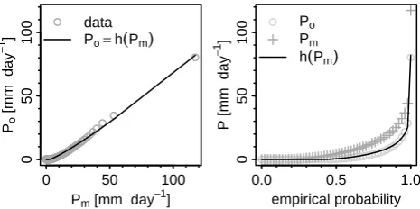
Fig. 1. Left: quantile–quantile plot of observed (Po) and modelled

(Pm) precipitation in Geiranger, Norway, as well as a

transforma-tion (Po=h(Pm)) that is used to map the modelled onto observed

quantiles. Right: empirical CDF of observed, modelled and trans-formed (h(Pm)) precipitation.

of the variable of interest is known, the transformation is defined as

Po =Fo−1(Fm(Pm)) , (2)

whereFmis the CDF ofPmandFo−1is the inverse CDF (or

quantile function) corresponding toPo.

Figure 1 illustrates statistical transformations for post pro-cessing RCM output using observed and modelled daily pre-cipitation rates from Geiranger, in the fjords of western Nor-way. Modelled precipitation was extracted from a HIRHAM RCM simulation with 25 km resolution (Førland et al., 2009, 2011) forced with the ERA40 reanalysis (Uppala et al., 2005) on a model domain covering Norway and the Nordic Arctic. The left panel shows the quantile–quantile plot of observed and modelled precipitation as well as the best fit of an ar-bitrary functionh that is used to approximate the transfor-mation. The right panel shows the corresponding empirical CDF of observed and modelled values as well as the trans-formed modelled values. The practical challenge is to find a suitable approximation forhand different approaches have been suggested in the literature.

2.1 Distribution derived transformations

Statistical transformations can be achieved by using theoret-ical distributions to solve Eq. (2). This approach has seen wide application for adjusting modelled precipitation (e.g. Ines and Hansen, 2006; Li et al., 2010; Piani et al., 2010a; Teutschbein and Seibert, 2012). Most of these studies assume thatF is a mixture of the Bernoulli and the Gamma distribu-tion, where the Bernoulli distribution is used to model the probability of precipitation occurrence and the Gamma dis-tribution used to model precipitation intensities (e.g. Thom, 1968; Mooley, 1973; Cannon, 2008). In this study, fur-ther mixtures, e.g. the Bernoulli-Weibull, the Bernoulli-Log-normal and the Bernoulli-Exponential distributions (Cannon, 2012), are also assessed. The parameters of the distributions

are estimated by maximum likelihood methods for bothPo

andPmindependently.

2.2 Parametric transformations

The quantile–quantile relation (Fig. 1) can be modelled di-rectly using parametric transformations. Here, the suitability of the following parametric transformations was explored:

ˆ

Po =b Pm (3)

ˆ

Po =a +b Pm (4)

ˆ

Po =b Pmc (5)

ˆ

Po =b (Pm−x)c (6)

ˆ

Po =(a+b Pm)

1−e−(Pm−x)/τ ₍₇₎

where,Pˆoindicates the best estimate ofPoanda,b,c,xand

τ are free parameters that are subject to calibration. The sim-ple scaling (Eq. 3) is regularly used to adjust precipitation from RCM (see Maraun et al., 2010, and references therein) and closely related to local intensity scaling (Schmidli et al., 2006; Widmann et al., 2003). The transformations Eq. (4) to Eq. (7) were all used by Piani et al. (2010b) and some of them have been further explored in follow up studies (Do-sio and Paruolo, 2011; Rojas et al., 2011). Following Pi-ani et al. (2010b), all parametric transformations were fitted to the fraction of the CDF corresponding to observed wet days (Po>0) by minimising the residual sum of squares.

Modelled values corresponding to the dry part of the ob-served empirical CDF were set to zero. Note, that the res-olution of the precipitation observations used in this study (see Sect. 3) is 0.1 mm day−1 which implies a threshold of

≤0.1 mm day−1.

2.3 Nonparametric transformations

2.3.1 Empirical quantiles (QUANT)

A common approach is to solve Eq. (2) using the empiri-cal CDF of observed and modelled values instead of assum-ing parametric distributions (e.g. Panofsky and Brier, 1968; Wood et al., 2004; Reichle and Koster, 2004; Bo´e et al., 2007; Themeßl et al., 2011, 2012). Following the procedure of Bo´e et al. (2007), the empirical CDFs are approximated using tables of empirical percentiles. Values in between the percentiles are approximated using linear interpolation. If new model values (e.g. from climate projections) are larger than the training values used to estimate the empirical CDF, the correction found for the highest quantile of the training period is used (Bo´e et al., 2007; Themeßl et al., 2012). 2.3.2 Smoothing splines (SSPLIN)

splines (e.g. Hastie et al., 2001), although other nonparamet-ric methods may be equally efficient. Like for the parametnonparamet-ric transformations (Sect. 2.2), the smoothing spline is only fit to the fraction of the CDF corresponding to observed wet days and modelled values below this are set to zero. The smooth-ing parameter of the spline is identified by means of gener-alised cross-validation.

3 Data and implementation

The suitability of the different statistical transformations to correct model precipitation from the HIRHAM RCM forced with the ERA40 reanalysis was tested using observed daily precipitation rates of 82 stations in Norway, all covering the 1960–2000 time interval. The methods were implemented in the R language (R Development Core Team, 2011) and bun-dled in the packageqmap, which is available on the Compre-hensive R Archive Network (http://www.cran.r-project.org/).

4 Quantifying performance

To assess the performance of the different methods, a set of scores is needed that quantifies the similarity of the observed and the (corrected) modelled empirical CDF. Previously used scores include overall measures, such as the root mean square error (Piani et al., 2010b) or the Kolmogorov-Smirnov two sample statistic (Dosio and Paruolo, 2011). Other suggested scores assess specific moments of the distribution includ-ing the mean (Engen-Skaugen, 2007; Li et al., 2010; Do-sio and Paruolo, 2011; Themeßl et al., 2011; Turco et al., 2011; Teutschbein and Seibert, 2012), the standard deviation (Engen-Skaugen, 2007; Li et al., 2010; Themeßl et al., 2011; Teutschbein and Seibert, 2012) and the skewness (Li et al., 2010). A variety of further scores are based on the compar-ison of the frequency of days with precipitation (Schmidli et al., 2006, 2007; Themeßl et al., 2011) and the magni-tude of selected (mostly high) percentiles (Schmidli et al., 2006, 2007; Li et al., 2010; Themeßl et al., 2011; Teutschbein and Seibert, 2012). All these scores are either presented as maps or as spatial averages, which facilitate a quantitative comparison of methods.

4.1 Skill scores

One limitation of the scores above is that they can often not be summarised into one overall measure, e.g. due to differ-ent physical units or lack of normalisation. This renders a global evaluation, combining the advantages and drawbacks of different methods, difficult. Therefore, this study suggests a novel set of scores that aims at a global evaluation, while keeping track of many relevant properties of the distribution. Overall performance is measured using the mean absolute er-ror (MAE) between the observed and the corrected empirical CDF. To assess the performance for more specific properties,

for example related to the fraction of dry days, average in-tensities or precipitation extremes, further scores are needed. Here these properties are assessed using MAE0.1, MAE0.2,

. . ., MAE1.0, the mean absolute errors computed for equally

spaced probability intervals of the observed empirical CDF. The subscript indicates the upper bounds of 0.1 wide prob-ability intervals. MAE0.1, for example, evaluates differences

in the dry part of the distribution, indicating discrepancies in the number of wet days. Similarly, MAE1.0indicates

dif-ferences in the magnitude of the most extreme events. Note also that MAE can be computed as the mean of MAE0.1,

MAE0.2, . . ., MAE1.0, which illustrates the consistency of

these measures.

Statistical transformations, as any statistical technique, quietly assume that the modelled relation holds if confronted with new data. In the context of climate impact assessment this assumption is critical as it has to be expected that cli-mate variables exceed the observed range in future periods. Further, highly adaptable methods, such as the nonparamet-ric techniques used in this study, are prone to over fitting the data. Both issues require that model error is quantified using data that have not been used for calibration. A standard tech-nique for this task is cross-validation (CV) (e.g. Hastie et al., 2001) which has been previously applied for evaluating sta-tistical downscaling techniques (e.g. Themeßl et al., 2011, 2012). Here a 10-fold CV was employed to produce unbi-ased estimates of MAE and MAE0.1, MAE0.2,. . ., MAE1.0.

First the data are split into 10 subsamples of continuous time intervals. The model is then calibrated using the data with one of the subsamples being removed. MAE and MAE0.1,

MAE0.2,. . ., MAE1.0are then estimated using the subsample

that was not used for calibration. This procedure is repeated for each subsample and results in 10 estimates of model er-ror. The mean of these 10 error estimates, the so called mean cross-validation error, is reported. In the remainder of this ar-ticle MAE and MAE0.1, MAE0.2,. . ., MAE1.0always refers

to the mean cross-validation error to ease formulation. 4.2 Ranking of methods

In order to obtain a global comparison of the efficiency of the different methods their performance was ranked, closely fol-lowing the procedure suggested by Reichler and Kim (2008). In a first step, relative errors are computed for each method by dividing the spatial averages of MAE and MAE0.1,

MAE0.2,. . ., MAE1.0by the corresponding scores of the

●●●● ● ● ● ● ● ● ● ● ● ● ● ● ● ● ● ● ● ● ● ● ● ● ● ● ● ● ● ● ● ● ● ●● ● ● ● ●● ● ● ● ● ● ● ● ●● ● ● ● ● ● ● ●● ● ● ●● ● ●●● ● ● ● ● ●● ● ● ● ● ● ● ● ● ● none ●●●● ● ● ● ● ● ● ● ● ● ● ● ● ● ● ● ● ● ● ● ● ● ● ● ● ● ● ● ● ● ● ● ●● ● ● ● ●● ● ● ● ● ● ● ● ● ● ● ● ● ● ● ● ●● ● ● ●● ● ●●● ● ● ● ● ●● ● ● ● ● ● ● ● ● ● BernExp ●●●● ● ● ● ● ● ● ● ● ● ● ● ● ● ● ● ● ● ● ● ● ● ● ● ● ● ● ● ● ● ● ● ●● ● ● ● ●● ● ● ● ● ● ● ● ●● ● ● ● ● ● ● ●● ● ● ●● ● ●●● ● ● ● ● ●● ● ● ● ● ● ● ● ● ● BernLogNorm ●●●● ● ● ● ● ● ● ● ● ● ● ● ● ● ● ● ● ● ● ● ● ● ● ● ● ● ● ● ● ● ● ● ●● ● ● ● ●● ● ● ● ● ● ● ● ●● ● ● ● ● ● ● ●● ● ● ●● ● ●●● ● ● ● ● ●● ● ● ● ● ● ● ● ● ● BernGamma ●●●● ● ● ● ● ● ● ● ● ● ● ● ● ● ● ● ● ● ● ● ● ● ● ● ● ● ● ● ● ● ● ● ●● ● ● ● ●● ● ● ● ● ● ● ● ● ● ● ● ● ●● ● ●● ● ● ●● ● ●●● ● ● ● ● ●● ● ● ● ● ● ● ● ● ● BernWeibull ●●●● ● ● ● ● ● ● ● ● ● ● ● ● ● ● ● ● ● ● ● ● ● ● ● ● ● ● ● ● ● ● ● ●● ● ● ● ●● ● ● ● ● ● ● ● ●● ● ● ● ●● ● ●● ● ● ●● ● ●●● ● ● ● ● ●● ● ● ● ● ● ● ● ● ●

Po=bPm

●●●● ● ● ● ● ● ● ● ● ● ● ● ● ● ● ● ● ● ● ● ● ● ● ● ● ● ● ● ● ● ● ● ●● ● ● ● ●● ● ● ● ● ● ● ● ●● ● ● ● ● ● ●●● ● ● ●● ● ●●● ● ● ● ● ●● ● ● ● ● ● ● ● ● ●

Po=a+bPm

●●●● ● ● ● ● ● ● ● ● ● ● ● ● ● ● ● ● ● ● ● ● ● ● ● ● ● ● ● ● ● ● ● ●● ● ● ● ●● ● ● ● ● ● ● ● ● ● ● ● ● ●● ●●● ● ● ●● ● ●●● ● ● ● ● ●● ● ● ● ● ● ● ● ● ●

Po=bPm

c ●●●● ● ● ● ● ● ● ● ● ● ● ● ● ● ● ● ● ● ● ● ● ● ● ● ● ● ● ● ● ● ● ● ●● ● ● ● ●● ● ● ● ● ● ● ● ●● ● ● ● ●● ●●● ● ● ●● ● ●●● ● ● ● ● ●● ● ● ● ● ● ● ● ● ●

Po=b(Pm−x)c

●●●● ● ● ● ● ● ● ● ● ● ● ● ● ● ● ● ● ● ● ● ● ● ● ● ● ● ● ● ● ● ● ● ●● ● ● ● ●● ● ● ● ● ● ● ● ●● ● ● ● ● ● ● ●● ● ● ●● ● ●●● ● ● ● ● ●● ● ● ● ● ● ● ● ● ●

Po=(a+bPm)(1−e−(Pm−x)τ)

●●●● ● ● ● ● ● ● ● ● ● ● ● ● ● ● ● ● ● ● ● ● ● ● ● ● ● ● ● ● ● ● ● ●● ● ● ● ●● ● ● ● ● ● ● ● ● ● ● ● ● ●● ●●● ● ● ●● ● ●●● ● ● ● ● ●● ● ● ● ● ● ● ● ● ● QUANT ●●●● ● ● ● ● ● ● ● ● ● ● ● ● ● ● ● ● ● ● ● ● ● ● ● ● ● ● ● ● ● ● ● ●● ● ● ● ●● ● ● ● ● ● ● ● ●● ● ● ● ●● ●●● ● ● ●● ● ●●● ● ● ● ● ●● ● ● ● ● ● ● ● ● ● SSPLINE

0.1 1 5

MAE [mm day−1]

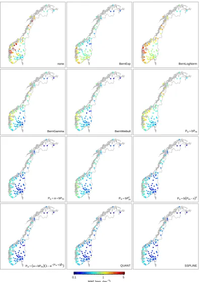
Fig. 2. Mean absolute error (MAE) between the observed and modelled empirical CDF for different statistical transformations, estimated

M

A

E

M

A

E0.1

M

A

E0.2

M

A

E0.3

M

A

E0.4

M

A

E0.5

M

A

E0.6

M

A

E0.7

M

A

E0.8

M

A

E0.9

M

A

E1

.0

0

2

4

6

8

●

● ● ● ● ●

● ●

● ●

●

●

● ● ● ●

● ●

● _●

● ●

M

A

E

[

m

m

d

a

y

−

1 ]

●

●

none BernExp BernLogNorm BernGamma BernWeibull Po=bPm

Po=a+bPm

Po=bPm c

Po=b(Pm−x)c

Po=(a+bPm)(1−e−(Pm−x)τ)

QUANT SSPLINE

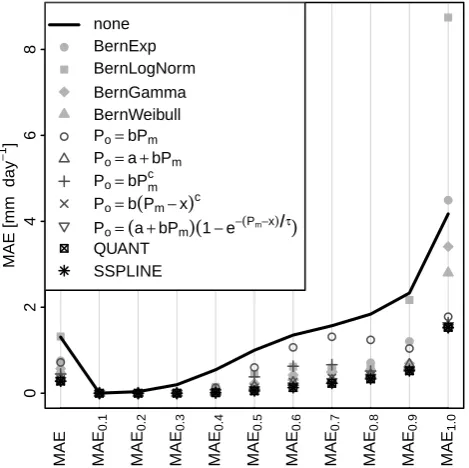
Fig. 3. Total mean absolute error (MAE) and the mean

abso-lute error for specific probability intervals (MAE0.1, MAE0.2,. . .,

MAE1.0), averaged over all stations.

5 Performance

The MAE for all stations and all methods under consider-ation is shown in Fig. 2. For the uncorrected model output MAE has pronounced geographic variations. The largest er-rors are found along the west coast, where the model cannot resolve the orographic effect on precipitation with sufficient detail. Most methods reduce the error and even out some of its spatial variability. An exception is the transformation based on the Bernoulli-Log-normal distribution, which does not lead to any visible improvements. The largest improve-ments are achieved by parametric and nonparametric trans-formations, especially along the west coast.

The MAE and MAE0.1, MAE0.2, . . ., MAE1.0 averaged

over all stations are shown in Fig. 3. Most methods reduce both the total MAE as well as the MAE for the percentile in-tervals. The absolute improvements are in most cases largest for the upper part of the CDF (p≥0.5). Note however, that two of the distribution derived transformations (Bernoulli-Exponential and Bernoulli-Log-normal) increase the error for the most extreme values. In the lower part of the CDF, the absolute improvements are generally smaller, owing to the small (often zero) precipitation rates.

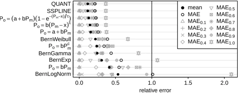
Figure 4 shows the ranking of the methods, based on the mean of the relative error (black dots). The hollow sym-bols show the relative errors for the total MAE and MAE0.1,

MAE0.2, . . ., MAE1.0. The two nonparametric methods

SSPLINE and QUANT have on average the best skill in re-ducing systematic errors, also for very high (extreme) per-centiles, being in line with other studies (Themeßl et al.,

2011; Teutschbein and Seibert, 2012). The success of the nonparametric transformations is likely related to their flexi-bility as they do not rely on any predetermined function. This flexibility allows good fits to any quantile–quantile relation. As for all highly adaptable methods with many degrees of freedom, over fitting may be a concern. Recall, however, that all scores are estimated using cross-validation, and that the estimated model error is independent from the data used for calibration. This suggests that over fitting is no major prob-lem if there are sufficient data. Nevertheless, over fitting may be an issue if the nonparametric transformations are cali-brated using small data samples, i.e. time series that cover only a short period. Similarly it cannot be ruled out that the methods perform badly if the projected climatic conditions differ substantially from the calibration period.

The large spread in performance of parametric transforma-tions is likely related to the flexibility of the different func-tions. Parametric transformations with three or more free pa-rameters (Eqs. 6 and 7) are almost as efficient as their non-parametric counterparts. Transformations with less flexibil-ity, in particular the simple scaling function (Eq. 3), do have worse performance.

The distribution derived transformations rank on average lowest. The best ranking distribution derived transformation is based on the Bernoulli-Weibull distribution. The transfor-mation derived from the Bernoulli-Log-normal distribution has the lowest performance of all considered methods. Note also that all distribution derived transformations have par-ticularly low performance with respect to the extreme part of the distribution. The low performance of distribution de-rived transformation may seem somewhat surprising, given the theoretical elegance of this approach. This is likely re-lated to the fact that the parameters of the distributions are identified forPoandPmseparately, which enables good

ap-proximations of the distributions ofPoandPmbut does not

necessarily optimise the statistical transformation as defined in Eq. (1).

6 Possible limitations of statistical transformations for post-processing RCM putput

●

●

●

●

●

●

●

●

●

●

● ●

●

●

●

●

●

●

●

●

●

● ●

●

●

●

●

●

●

●

●

●

● BernLogNorm

Po=bPm

BernExp BernGamma

Po=bPm

c BernWeibull

Po=a+bPm

Po=b(Pm−x)c

Po=

(

)

SSPLINE QUANT

0.0 0.5 1.0 1.5 2.0

●

●

● mean MAE

MAE0.1

MAE0.2

MAE0.3

MAE0.4

MAE0.5

MAE0.6

MAE0.7

MAE0.8

MAE0.9

MAE1.0

relative error

Fig. 4. Performance ranking of statistical transformations used for post-processing RCM output. Relative error (hollow symbols) is defined

as the MAE of each method divided by the MAE of the uncorrected model output. The mean relative error (black dots) is used to rank the different methods.

indicate the stability of the methods. Further, numerical ex-periments on the global scale have shown that uncertainty re-lated to the choice of calibration period is small compared to uncertainties related to choice of climate model and emission scenario (Chen et al., 2011a).

A related concern is the impact of post processing tech-niques on the climate change signal. Empirical investigations indicate that the impact of statistical transformations on the projected changes in mean conditions is comparably small but may systematically alter changes in nonlinearly derived measures, including characteristics of extreme events (The-meßl et al., 2011). Similarly statistical transformations and other bias correction techniques may have side effects on further statistical properties even if they are not explicitly de-signed to change these. Examples include changes in the am-plitude of low frequency variability (Haerter et al., 2011) or the modification of measures characterising temporal persis-tence (Johnson and Sharma, 2012, 2011). However, whether these side effects are considered to be beneficial (correction of higher order properties), adverse (introduction of artifacts) or neutral (e.g. if only mean values are of interest) depends on particular applications and has to be evaluated on a case to case basis.

7 Conclusions

The three approaches using statistical transformation to post-process RCM output that were assessed in this paper differ substantially with respect to their underlying assumptions, despite the fact that they are all designed to transform RCM output such that its empirical distribution matches the distri-bution of observed values. A real-world evaluation of a wide range of statistical transformations showed that most of them are capable to remove biases in RCM precipitation. Despite this overall success, it was also demonstrated that the per-formance of the methods differ substantially. Therefore, we

stress that these techniques should not be applied without checking their suitability for the data under consideration. The methods with the best skill in reducing biases from RCM precipitation through the entire range of the distribution are all classified as nonparametric transformations. These have the additional advantage that they can be applied without spe-cific assumptions about the distribution of the data and are thus recommended for most applications of statistical bias correction.

Appendix A

Note on terminology

the presented techniques without interfering with previously used terminology.

Acknowledgements. This research was co-funded by the MIST

project, a collaboration between the hydro-power company Statkraft and the Norwegian Meteorological Institute.

Edited by: J. Seibert

References

Angus, J. E.: The Probability Integral Transform and Related Re-sults, SIAM Review, 36, 652–654, 1994.

Ashfaq, M., Bowling, L. C., Cherkauer, K., Pal, J. S., and Diffen-baugh, N. S.: Influence of climate model biases and daily-scale temperature and precipitation events on hydrological impacts as-sessment: A case study of the United States, J. Geophys. Res., 115, D14116, doi:10.1029/2009JD012965, 2010.

Bo´e, J., Terray, L., Habets, F., and Martin, E.: Statistical and dynamical downscaling of the Seine basin climate for hydro-meteorological studies, Int. J. Climatol., 27, 1643–1655, doi:10.1002/joc.1602, 2007.

Cannon, A. J.: Probabilistic Multisite Precipitation Downscaling by an Expanded Bernoulli-Gamma Density Network, J. Hydrome-teorol., 9, 1284–1300, doi:10.1175/2008JHM960.1, 2008. Cannon, A. J.: Neural networks for probabilistic environmental

pre-diction: Conditional Density Estimation Network Creation and Evaluation (CaDENCE) in R, Comput. Geosci., 41, 126–135, doi:10.1016/j.cageo.2011.08.023, 2012.

Chen, C., Haerter, J. O., Hagemann, S., and Piani, C.: On the con-tribution of statistical bias correction to the uncertainty in the projected hydrological cycle, Geophys. Res. Lett., 38, L20403, doi:10.1029/2011GL049318, 2011a.

Chen, J., Brissette, F. P., and Leconte, R.: Uncertainty of downscaling method in quantifying the impact of cli-mate change on hydrology, J. Hydrol., 401, 190–202, doi:10.1016/j.jhydrol.2011.02.020, 2011b.

Christensen, J. H., Boberg, F., Christensen, O. B., and Lucas-Picher, P.: On the need for bias correction of regional climate change projections of temperature and precipitation, Geophys. Res. Lett., 35, L20709, doi:10.1029/2008GL035694, 2008. Dosio, A. and Paruolo, P.: Bias correction of the ENSEMBLES

high-resolution climate change projections for use by impact models: Evaluation on the present climate, J. Geophys. Res., 116, D16106, doi:10.1029/2011JD015934, 2011.

Engen-Skaugen, T.: Refinement of dynamically downscaled pre-cipitation and temperature scenarios, Climatic Change, 84, 365– 382, doi:10.1007/s10584-007-9251-6, 2007.

Førland, E. J., Benestad, R. E., Flatø, F., Hanssen-Bauer, I., Haugen, J. E., Isaksen, K., Sorteberg, A., and ˚Adlandsvik, B.: Climate development in North Norway and the Svalbard region during 1900–2100, Tech. Rep. 128, Norwegian Polar Institute, available at: http://www.npolar.no (last access: 15 May 2012), 2009. Førland, E. J., Benestad, R., Hanssen-Bauer, I., Haugen, J. E., and

Skaugen, T. E.: Temperature and Precipitation Development at Svalbard 1900–2100, Advances in Meteorology, 2011, 893790, doi:10.1155/2011/893790, 2011.

Haerter, J. O., Hagemann, S., Moseley, C., and Piani, C.: Cli-mate model bias correction and the role of timescales, Hy-drol. Earth Syst. Sci., 15, 1065–1079, doi:10.5194/hess-15-1065-2011, 2011.

Hastie, T., Tibshirani, R., and Friedman, J. H.: The Elements of Sta-tistical Learning, Springer, 2001.

Ines, A. V. and Hansen, J. W.: Bias correction of daily GCM rainfall for crop simulation studies, Agr. Forest Meteorol., 138, 44–53, doi:10.1016/j.agrformet.2006.03.009, 2006.

Johnson, F. and Sharma, A.: Accounting for interannual vari-ability: A comparison of options for water resources climate change impact assessments, Water Resour. Res., 47, W04508, doi:10.1029/2010WR009272, 2011.

Johnson, F. and Sharma, A.: A nesting model for bias correc-tion of variability at multiple time scales in general circula-tion model precipitacircula-tion simulacircula-tions, Water Resour. Res., 48, W01504, doi:10.1029/2011WR010464, 2012.

Li, H., Sheffield, J., and Wood, E. F.: Bias correction of monthly precipitation and temperature fields from Intergovern-mental Panel on Climate Change AR4 models using equidis-tant quantile matching, J. Geophys. Res., 115, D10101, doi:10.1029/2009JD012882, 2010.

Maraun, D., Wetterhall, F., Ireson, A. M., Chandler, R. E., Kendon, E. J., Widmann, M., Brienen, S., Rust, H. W., Sauter, T., The-meßl, M., Venema, V. K. C., Chun, K. P., Goodess, C. M., Jones, R. G., Onof, C., Vrac, M., and Thiele-Eich, I.: Precipita-tion downscaling under climate change: Recent developments to bridge the gap between dynamical models and the end user, Rev. Geophys., 48, RG3003, doi:10.1029/2009RG000314, 2010. Mooley, D. A.: Gamma Distribution Probability Model

for Asian Summer Monsoon Monthly Rainfall, Mon. Weather Rev., 101, 160–176, doi:10.1175/1520-0493(1973)101<0160:GDPMFA>2.3.CO;2, 1973.

Panofsky, H. W. and Brier, G. W.: Some Applications of Statistics to Meteorology, The Pennsylvania State University Press, Philadel-phia, 1968.

Piani, C., Haerter, J., and Coppola, E.: Statistical bias correction for daily precipitation in regional climate models over Europe, Theor. Appl. Climatol., 99, 187–192, doi:10.1007/s00704-009-0134-9, 2010a.

Piani, C., Weedon, G., Best, M., Gomes, S., Viterbo, P., Hage-mann, S., and Haerter, J.: Statistical bias correction of global simulated daily precipitation and temperature for the appli-cation of hydrological models, J. Hydrol., 395, 199–215, doi:10.1016/j.jhydrol.2010.10.024, 2010b.

R Development Core Team: R: A Language and Environment for Statistical Computing, R Foundation for Statistical Computing, Vienna, Austria, available at: http://www.R-project.org/ (last ac-cess: 15 May 2012), 2011.

Rauscher, S., Coppola, E., Piani, C., and Giorgi, F.: Resolu-tion effects on regional climate model simulaResolu-tions of sea-sonal precipitation over Europe, Clim. Dynam., 35, 685–711, doi:10.1007/s00382-009-0607-7, 2010.

Reichle, R. H. and Koster, R. D.: Bias reduction in short records of satellite soil moisture, Geophys. Res. Lett., 31, L19501, doi:10.1029/2004GL020938, 2004.

Rojas, R., Feyen, L., Dosio, A., and Bavera, D.: Improving pan-European hydrological simulation of extreme events through sta-tistical bias correction of RCM-driven climate simulations, Hy-drol. Earth Syst. Sci., 15, 2599–2620, doi:10.5194/hess-15-2599-2011, 2011.

Schmidli, J., Frei, C., and Vidale, P. L.: Downscaling from GCM precipitation: a benchmark for dynamical and statis-tical downscaling methods, Int. J. Climatol., 26, 679–689, doi:10.1002/joc.1287, 2006.

Schmidli, J., Goodess, C. M., Frei, C., Haylock, M. R., Hundecha, Y., Ribalaygua, J., and Schmith, T.: Statistical and dynamical downscaling of precipitation: An evaluation and comparison of scenarios for the European Alps, J. Geophys. Res., 112, D04105, doi:10.1029/2005JD007026, 2007.

Sunyer, M., Madsen, H., and Ang, P.: A comparison of different regional climate models and statistical downscaling methods for extreme rainfall estimation under climate change, Atmos. Res., 103, 119–128, doi:10.1016/j.atmosres.2011.06.011, 2012. Teutschbein, C. and Seibert, J.: Regional Climate Models for

Hy-drological Impact Studies at the Catchment Scale: A Review of Recent Modeling Strategies, Geography Compass, 4, 834–860, doi:10.1111/j.1749-8198.2010.00357.x, 2010.

Teutschbein, C. and Seibert, J.: Bias correction of regional climate model simulations for hydrological climate-change impact stud-ies: Review and evaluation of different methods, J. Hydrol., 16, 12–29, doi:10.1016/j.jhydrol.2012.05.052, 2012.

Themeßl, M. J., Gobiet, A., and Leuprecht, A.: Empirical-statistical downscaling and error correction of daily precipitation from regional climate models, Int. J. Climatol., 31, 1530–1544, doi:10.1002/joc.2168, 2011.

Themeßl, M. J., Gobiet, A., and Heinrich, G.: Empirical-statistical downscaling and error correction of regional climate models and its impact on the climate change signal, Climatic Change, 112, 449–468, doi:10.1007/s10584-011-0224-4, 2012.

Thom, H. C. S.: Approximate convolution of the gamma and mixed gamma distributions, Mon. Weather Rev., 96, 883–886, doi:10.1175/1520-0493(1968)096<0883:ACOTGA>2.0.CO;2, 1968.

Turco, M., Quintana-Segu´ı, P., Llasat, M. C., Herrera, S., and Guti´errez, J. M.: Testing MOS precipitation downscaling for ENSEMBLES regional climate models over Spain, J. Geophys. Res., 116, D18109, doi:10.1029/2011JD016166, 2011.

Uppala, S. M., K˚allberg, P. W., Simmons, A. J., Andrae, U., Bech-told, V. D. C., Fiorino, M., Gibson, J. K., Haseler, J., Hernandez, A., Kelly, G. A., Li, X., Onogi, K., Saarinen, S., Sokka, N., Al-lan, R. P., Andersson, E., Arpe, K., Balmaseda, M. A., Beljaars, A. C. M., Berg, L. V. D., Bidlot, J., Bormann, N., Caires, S., Chevallier, F., Dethof, A., Dragosavac, M., Fisher, M., Fuentes, M., Hagemann, S., H´olm, E., Hoskins, B. J., Isaksen, L., Janssen, P. A. E. M., Jenne, R., Mcnally, A. P., Mahfouf, J.-F., Morcrette, J.-J., Rayner, N. A., Saunders, R. W., Simon, P., Sterl, A., Tren-berth, K. E., Untch, A., Vasiljevic, D., Viterbo, P., and Woollen, J.: The ERA-40 reanalysis, Q. J. Roy. Meteor. Soc., 131, 2961– 3012, doi:10.1256/qj.04.176, 2005.

Widmann, M., Bretherton, C. S., and Salath´e, E. P.: Sta-tistical Precipitation Downscaling over the Northwestern United States Using Numerically Simulated Precipitation as a Predictor, J. Climate, 16, 799–816, doi:10.1175/1520-0442(2003)016<0799:SPDOTN>2.0.CO;2, 2003.

Winkler, J. A., Guentchev, G. S., Liszewska, M., Perdinan, and Tan, P.-N.: Climate Scenario Development and Applications for Lo-cal/Regional Climate Change Impact Assessments: An Overview for the Non-Climate Scientist – Part II: Considerations When Using Climate Change Scenarios, Geography Compass, 5, 301– 328, doi:10.1111/j.1749-8198.2011.00426.x, 2011a.

Winkler, J. A., Guentchev, G. S., Perdinan, Tan, P.-N., Zhong, S., Liszewska, M., Abraham, Z., Nied´zwied´z, T., and Ustrnul, Z.: Climate Scenario Development and Applications for Lo-cal/Regional Climate Change Impact Assessments: An Overview for the Non-Climate Scientist – Part I: Scenario Development Using Downscaling Methods, Geography Compass, 5, 275–300, doi:10.1111/j.1749-8198.2011.00425.x, 2011b.