Singularity sensitive gauge based radar rainfall adjustment methods for urban hydrological applications

www.hydrol-earth-syst-sci.net/19/4001/2015/ doi:10.5194/hess-19-4001-2015

© Author(s) 2015. CC Attribution 3.0 License.

Singularity-sensitive gauge-based radar rainfall adjustment

methods for urban hydrological applications

L.-P. Wang1, S. Ochoa-Rodríguez2, C. Onof2, and P. Willems1

1_{Hydraulics Laboratory, Katholieke Universiteit Leuven, 3001 Heverlee (Leuven), Belgium}

2_{Department of Civil and Environmental Engineering, Imperial College London, London, SW7 2AZ, UK} Correspondence to: L.-P. Wang ([email protected])

Received: 7 December 2014 – Published in Hydrol. Earth Syst. Sci. Discuss.: 6 February 2015 Revised: 3 August 2015 – Accepted: 14 September 2015 – Published: 29 September 2015

Abstract. Gauge-based radar rainfall adjustment techniques have been widely used to improve the applicability of radar rainfall estimates to large-scale hydrological mod-elling. However, their use for urban hydrological applica-tions is limited as they were mostly developed based upon Gaussian approximations and therefore tend to smooth off so-called “singularities” (features of a non-Gaussian field) that can be observed in the fine-scale rainfall structure. Over-looking the singularities could be critical, given that their distribution is highly consistent with that of local extreme magnitudes. This deficiency may cause large errors in the subsequent urban hydrological modelling. To address this limitation and improve the applicability of adjustment tech-niques at urban scales, a method is proposed herein which incorporates a local singularity analysis into existing adjust-ment techniques and allows the preservation of the singu-larity structures throughout the adjustment process. In this paper the proposed singularity analysis is incorporated into the Bayesian merging technique and the performance of the resulting singularity-sensitive method is compared with that of the original Bayesian (non singularity-sensitive) technique and the commonly used mean field bias adjustment. This test is conducted using as case study four storm events observed in the Portobello catchment (53 km2) (Edinburgh, UK) dur-ing 2011 and for which radar estimates, dense rain gauge and sewer flow records, as well as a recently calibrated urban drainage model were available. The results suggest that, in general, the proposed singularity-sensitive method can effec-tively preserve the non-normality in local rainfall structure, while retaining the ability of the original adjustment tech-niques to generate nearly unbiased estimates. Moreover, the ability of the singularity-sensitive technique to preserve the

non-normality in rainfall estimates often leads to better re-production of the urban drainage system’s dynamics, partic-ularly of peak runoff flows.

1 Introduction

Traditionally, urban hydrological applications have relied mainly upon rain gauge data as input. While rain gauges generally provide accurate point rainfall estimates near the ground surface, they cannot properly capture the spatial vari-ability of rainfall, which has a significant impact on the ur-ban hydrological system and thus on the modelling of urur-ban runoff (Gires et al., 2012; Schellart et al., 2012). Thanks to the development of radar technology, weather radar data have been playing an increasingly important role in urban hydrol-ogy (Krämer et al., 2007; Liguori et al., 2011). Radars can survey large areas and better capture the spatial variability of the rainfall, thus improving the short-term predictability of rainfall and flooding. However, the accuracy of radar mea-surements is in general insufficient, particularly in the case of extreme rainfall magnitudes (Einfalt et al., 2004, 2005). This is due to the fact that, instead of being a direct measurement, radar rainfall intensity is derived indirectly from measured radar reflectivity. As a result, both radar reflectivity measure-ments and the reflectivity–intensity conversion process are subject to multiple sources of error.

of corrections before they are converted into rainfall inten-sity, it is virtually impossible to have error-free reflectivity measurements. Second, the conversion between radar reflec-tivity (Z) and rainfall rate (R) uses the so-calledZ–R rela-tionship,Z=a Rb(Marshall and Palmer, 1948), whereaand bare variables generally deduced by physical approximation or empirical calibration. This can be theoretically linked to the rain drop size distribution, which varies for different rain-fall types. Operationally, a number of “static”Z–Rrelations are usually derived to generate radar rainfall rates for dif-ferent rainfall types (e.g. stratiform, convective and tropical storms), and the associated a andb variables are calibrated based upon long-term comparisons (Collier, 1986; Krajewski and Smith, 2002). However, in reality, it is almost impossi-ble to classify a single storm purely under a specific rain-fall type. Consequently, it is not entirely appropriate to use a staticZ–Rrelation to derive rainfall intensities, even for a single storm event. This has been confirmed by several stud-ies, which indicate that rain drop size distribution is a highly dynamic process and may significantly or suddenly change within a storm event (Smith et al., 2009; Ulbrich, 1983). Be-cause of this, the Z–R derived rainfall intensity cannot ef-fectively reflect the short-term dynamics of true rainfall in-tensities and may statistically compromise with intermediate rainfall intensities.

In order to overcome these drawbacks of radar rainfall es-timates while preserving their spatial description of rainfall fields, it is possible to dynamically adjust them using rain gauge measurements. Many studies on this subject have been carried out over the last few years, though most of them fo-cus on hydrological applications at large scales (Anagnostou and Krajewski, 1999; Fulton et al., 1998; Germann et al., 2006; Goudenhoofdt and Delobbe, 2009; Harrison et al., 2000, 2009; Seo and Smith, 1991; Thorndahl et al., 2014). Only few studies have examined the applicability of these adjustment techniques to urban-scale hydrological applica-tions and concluded that they can effectively reduce rain-fall bias, thus leading to improvements in the reproduction of hydrological outputs (Smith et al., 2007; Vieux and Bedi-ent, 2004; Villarini et al., 2010; Wang et al., 2013). How-ever, despite the improvements achieved with the current adjustment techniques, underestimation of storm peaks can still be seen after adjustment and this is particularly evident in the case of small drainage areas (such as those of urban catchments) and extreme rainfall magnitudes (Wang et al., 2012; Ochoa-Rodríguez et al., 2013). This may be due to the fact that the underlying adjustment techniques, mainly based upon Gaussian (first and/or second statistical moments) ap-proximations (Goudenhoofdt and Delobbe, 2009; Krajewski, 1987; Todini, 2001), cannot properly cope with the so-called “singularities” (which imply non-normality and often corre-spond to local extreme magnitudes) observed at small scales (Schertzer et al., 2013; Tchiguirinskaia et al., 2012). In fact, it is often the case that the radar image captures the spatial structure of striking local extremes (albeit the actual rainfall

depth/intensity may be inaccurate), but these structures are lost or smoothened throughout the merging process. This de-ficiency may cause large errors in the subsequent urban hy-drological modelling.

To address this limitation and improve the applicability of adjustment techniques at urban scales, a method is proposed herein which incorporates a local singularity (identification) analysis (Cheng et al., 1994; Schertzer and Lovejoy, 1987; Wang et al., 2012) into existing adjustment techniques and enables the preservation of the singularity structures through-out the adjustment process. The singularity-sensitive method is particularly intended to improve geostatistical-based merg-ing techniques (e.g. co-krigmerg-ing, Krajewski, 1987; Bayesian merging, Todini, 2001; kriging with external drift, Wacker-nagel, 2003 and conditional merging, Sinclair and Pegram, 2005), which seek to represent the spatial covariance struc-ture of the rainfall field or its errors by making use of the semi-variogram (Goudenhoofdt and Delobbe, 2009). Being a second-order tool, the semi-variogram cannot adequately capture higher-order features of the rainfall field, thus caus-ing these to be lost in the mergcaus-ing process.

The proposed singularity-sensitive method was initially developed and preliminarily tested in the reconstruction of a storm event which led to reported flooding in the Maida Vale area, Central London, in June 2009 (Wang and Onof, 2013; Wang et al., 2014). The radar rainfall product for this event showed strong and localised singularity struc-tures, but the accuracy of the actual estimates was poor. A dynamic gauge-based adjustment was conducted using the Bayesian data merging method (Todini, 2001), which in pre-vious studies had been shown to outperform other adjustment methods (Mazzetti and Todini, 2004; Wang et al., 2013). Nonetheless, for this particular event records from only a few rain gauge sites were available and these were located away from the area of interest and at points where less in-tense radar rainfall was observed. Under these circumstances, the aforementioned shortcomings associated with existing adjustment techniques became evident. The Bayesian data merging method proved inadequate as it smoothed out the singularity structures, which had the effect of considerably reducing the peak rainfall intensities. It was then that the singularity-sensitive method was devised and effectively in-corporated into the Bayesian merging technique. The result-ing sresult-ingularity-sensitive Bayesian mergresult-ing method led to rainfall fields which better preserved the spatial structure as captured by the radar and better reproduced peak rainfall in-tensities.

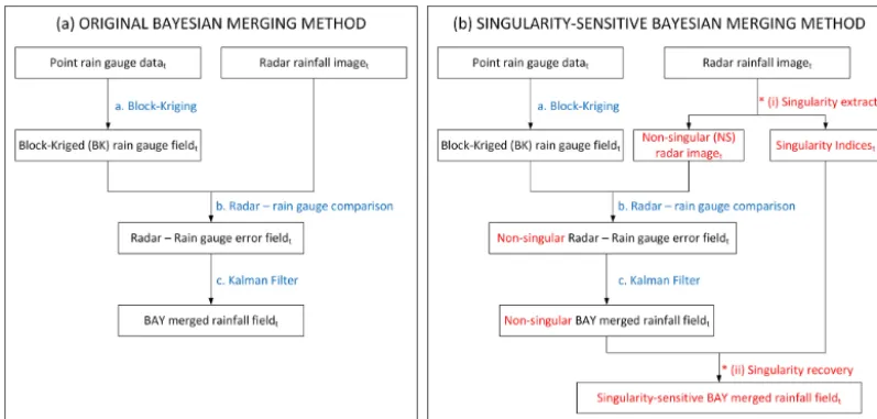
net-Figure 1. Schematics of (a) original Bayesian merging method (adapted from Fig. 2 in Mazzetti (2012)) and (b) singularity-sensitive

Bayesian merging method.

work of rain and flow gauges, as well as a recently calibrated urban drainage model were available.

The paper is organised as follows. In Sect. 2 a detailed explanation is provided of the theoretical development of the singularity-sensitive method, including the newly imple-mented numerical strategies. In Sect. 3 we present the case study, including a description of the study area and data set, the performance criteria used to evaluate the proposed methodology, and the results of the testing. Lastly, in Sect. 4 the main conclusions are presented and future work is dis-cussed.

2 Formulation of the singularity-sensitive Bayesian data merging method

Firstly, a description is provided of the two key techniques used in this paper: the Bayesian data merging method and the local singularity analysis. Afterwards, the proposed method for integrating these two techniques is explained. Intermedi-ate results of each of the steps described in this section, which help illustrate the main features of the proposed methodol-ogy, can be found in the Supplement.

2.1 Bayesian radar–rain gauge data merging method The Bayesian data merging method (BAY) is a dynamic ad-justment method (applied independently at each time step) intended for real-time applications (Todini, 2001). The derlying idea of this method is to analyse and quantify the un-certainty of rainfall estimates (in terms of error co-variance) from multiple data sources – in this case, radar and rain gauge sensors – and then combine these estimates in such a way that the overall (estimation) uncertainty is minimised. The BAY

merging method consists of the following steps (illustrated in Fig. 1a):

a. For each time stept, the point rain gauge (RG) mea-surements are interpolated into a synthetic rainfall field using the block kriging (BK) technique. The result of this step is an interpolated rain gauge rainfall field, with areal estimates at each radar grid location (y_tRG), and which are accompanied by the associated estimation er-ror co-variance function (V_εRG

t ), representing the uncer-tainty of rain gauge estimates.

b. The interpolated rain gauge rainfall field is compared against the radar field (y_tRD), based upon which a field of errors (estimated as the bias at each radar grid lo-cation:εRD_t =y_tRD−y_tRG) is obtained empirically. As-suming that areal rain gauge estimates are unbiased, the expectation value (µ_εRD

t ) and the co-variance function (V_εRD

t ) of this radar–rain gauge error field at each time step is used to represent, respectively, the mean bias and the uncertainty of radar estimates.

c. Using a Kalman filter (Kalman, 1960), the two rainfall fields are optimally combined such that the overall es-timation uncertainty is minimised. In the Kalman filter the radar data and the interpolated rain gauge estimates act, respectively, as “a priori estimate” and “measure-ment”. The degree of “uncertainty” of each type of es-timate constitutes a gain value (the so-called Kalman gain, Kt) at each radar grid location, and determines

Kt=V_εRD t

V_εRD t +VεtRG

−1

, (1)

and the optimally merged output, BAY (i.e. the a poste-riori estimatesy_t00in the Kalman filter) can be obtained from

y_t00=y_t0+Kt

y_tRG−y_t0, (2)

where y0_t is the “unbiased” radar rainfall estimate (i.e. y0_t=yRD_t −µ_εRD

t ) used as the a priori estimate in the Kalman filter.

It can be seen that the Kalman gain is a function of the co-variances of radar and rain gauge estimation er-rors. WhenV_εRD

t VεRGt (orKt

≈1, i.e. radar estimates have significantly higher uncertainty than the rain gauge ones), the radar estimates are less trustworthy and the output estimates will be very similar to the interpo-lated rain gauge field. In contrast, when V_εRG

t

V_εRD t (or Kt≈0), the output will be closer to the radar

esti-mates.

It is in steps b and c where the problems associated with the Bayesian merging technique, and geostatistical techniques in general, arise. The (second-order) co-variance function that these techniques employ to characterise radar–rain gauge er-rors cannot well capture local singularity structures. Instead, in second-order models singularities may be mistakenly re-garded as errors in the radar data, thus leading to higher esti-mated radar uncertainty,V_εRD

t . As a result, the radar data will be trusted less, leading to smoother merged outputs, which are closer to the interpolated rain gauge field.

2.2 Local singularity analysis

Various types of hazardous geo-processes, including precip-itation, often result in anomalous amounts of energy release or mass accumulation confined to narrow intervals in time and/or space. The property of anomalous amounts of energy release or mass accumulation is termed singularity and it is often associated with structures depicting fractality or multi-fractality (Agterberg, 2007; Cheng, 1999; Lovejoy and Man-delbrot, 1985; Schertzer and Lovejoy, 1987). Several math-ematical models and methodologies have been developed to respectively characterise and treat singularities. In this work, the local singularity analysis proposed by Cheng et al. (1994) has been adopted to identify and extract singularities form rainfall fields. Cheng’s method, which has been widely used for estimation of geo-chemical concentrations (Agterberg, 2007; Cheng and Zhao, 2011; Cheng et al., 1994), employs the definition of coarse Hölder exponent to characterise sin-gularities. According to this model, singularities are defined by the fact that the areal average measure (in this work, areal rainfall) centred on point x (taken as the centre of a radar pixel) varies as a power function of the area (Evertsz and

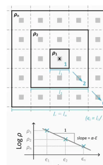
Figure 2. Schematic of the local singularity analysis (adapted from

Wang et al., 2014).

Mandelbrot, 1992). This power-law relationship can be for-mulated as an equation (Cheng et al., 1994):

ρ(x, )=c(x)α(x)−E, (3)

whereρ(x,)represents the density of measure (e.g. con-centration of geo-data; in the context of this paper, rainfall intensity) over a square area with side-lengthl and associ-ated scale(=l/L, whereLis the side-length of the largest square area under consideration) centred at a specific loca-tionx;c(x)is a constant value (in the context of this paper, a constant intensity value) atx;α(x)is the singularity index (or the coarse Hölder exponent); andE=2 is the Euclidean dimension of the plane.

A schematic of the estimation of the constant valuec(x) and singularity indexα(x)from gridded data is provided in Fig. 2. For a given pixel with centrex(centre of top plot in Fig. 2), the mean rainfall intensities at different spatial scales (centred inx) can be calculated (i.e. rainfall intensitiesρ1, ρ2, . . ., ρn, respectively at scales1,2, . . ., n). Then, the

c(x)andα(x)can be trusted only if a good linear relation is observed (i.e. if the scaling behaviour is well followed).

Going back to the definition of singularity, Eq. (3) consti-tutes a useful tool to decompose an areal rainfall intensity at a given locationxinto two components (Wang et al., 2012): (1) the background (or non-singular, NS) magnitude c(x), which is invariant as measuring scalechanges and is more approximately normal than the original field; and (2) a local “scaling” multiplier, the magnitude of which changes as the measuring scalechanges, according to the local singularity indexα(x). Whenα(x) <2, the rainfall magnitude strikingly increases as the measuring scale decreases (namely local enrichment); this corresponds to a “peak” singularity. In con-trast, when α(x) >2, the rainfall magnitude decreases as decreases (i.e. local depletion), and it is therefore a “trough” singularity. Whenα(x)=2, there is no singularity: the rain-fall intensityρ(x,)within a×area remains the same as scale changes (i.e.ρ(x,)=c(x)).

In practice however, there is a drawback to this local sin-gularity analysis. Because it carries out a “local” analysis, the singularity exponents are usually obtained from a small number of data samples. This increases the uncertainty of the estimation ofα(x). The consequence of this drawback is that the singularity is incorrectly estimated or incompletely extracted; therefore,c(x)is an unreliable or incomplete non-singular value. To circumvent this, two numerical strategies were employed in this study. The first one involves constrain-ing the value of the estimated sconstrain-ingularity exponents within a certain range. This can avoid obtaining unreasonably large or small singularity exponents. A number of ranges, sym-metric to the non-singular condition (i.e.α(x)=2), were se-lected for testing. They are (from the widest to narrowest intervals): SIN1=[0, 4], SIN2=[0.5, 3.5], SIN3=[1, 3], SIN4=[1.5, 2.5] and SIN5=[1.75, 2.25]. These “truncated” singularity ranges were empirically chosen according to the authors’ experience and the fact that the distribution ofα(x) is seldom largely skewed to a specific side of α(x)=2. It can be generally expected that, the wider the range is, the more singularity information (both local enrichment and de-pletion) from the radar images is taken into account in the merging process. The impact of different singularity ranges in rainfall estimation and hydraulic simulation is further dis-cussed in Sect. 3.3.

The second numerical strategy is to decompose the rainfall field using an iterative procedure (Agterberg, 2012b; Chen et al., 2007):

c(k−1)(x)=c(k)(x)α(k)(x)−E, (4) where the iterative index k=,0,1,2, . . ., n. As k=0, c(−1)(x)=ρ(x, ) (i.e. the original value) and c(0)(x) is the “calculated non-singular” value from the first iteration, which is equal to c(x) from the non-iterative calculation above (Eq. 3). Thisc(0)(x)is then used as the left-hand-side value of Eq. (4) to calculate the “non-singular” value at the

next iteration, and so on. Substituting Eq. (4) into Eq. (3), one can obtain an iterative local singularity analysis equation: ρ(x, )=c∗(x)α∗(x)−E, (5) where

(

c∗(x)=c(n)(x) α∗(x)=α(0)(x)+Pn

k=1 α(k)(x)−E

. (6)

The criterion to terminate the iteration procedure is when α(k)(x)≈E (which is equivalent to c(k−1)(x)≈c(k)(x)). That means the singularity components have been clearly re-moved from the data.

Moreover, in this work a spatial-scale range of 1–9 km, which results in a total of five rainfall intensity samples (at scales 1, 3, 5, 7 and 9 km), was used in the singularity anal-ysis. This range was selected for two main reasons. Firstly, our analyses revealed that a good linear behaviour was gener-ally observed within this scale range, while small-scale struc-tures were still preserved in the resulting rainfall product. As such, the selected spatial scale range was deemed to repre-sent a good balance between estimation uncertainty (which depends upon the number of samples employed in the cal-culations) and local feature preservation. Secondly, a scaling break at approximately 8–16 km has been reported in studies in which 1 km radar rainfall data were analysed (Gires et al., 2012; Tchiguirinskaia et al., 2012). This means that the rain-fall data at spatial-scale regimes ranging from 1 to 8–16 km comply with the same or similar statistical or physical be-haviour. This scaling range has also been used in other appli-cations to represent relatively local characteristics of rainfall fields (Bowler et al., 2006).

Lastly, a 10-iteration singularity analysis was applied in order to ensure that most of the singularity exponents could be extracted. The downside of conducting many iterations is the longer computational time, which may be an issue for real-time applications. Nonetheless, in practice, approxi-mately 4–6 iterations are sufficient for effectively removing most of the singularity.

2.3 Incorporation of the local singularity analysis into the Bayesian merging method

Figure 3. Portobello catchment (a) general location; (b) sensor location, sewer network and radar grid over the catchment. Flow gauges

FM 3, 10, 14 and 19 (the circled round markers in (b), respectively located at the up-, mid- and downstream parts of the catchment) are particularly selected for visual inspection in Sect. 3.3.2.

value of the NS-BAY field by the following ratio:

r(x)=α∗(x)−E (7)

which corresponds to the ratio difference between the orig-inal radar field (RD) and the non-singular radar field (NS-RD). In this way, a singularity-sensitive merged field (SIN), which better retains the local singularity structures embedded in the original RD field, is obtained.

It is worth noting that the proposed singularity-sensitive merging method does not always increase the reliability of RD estimates. Such increase only happens when the RD es-timates exhibit high singularity and thus cannot be well han-dled using Gaussian approximations.

A particular phenomenon which may cause problems in the application of the proposed methodology and is therefore worth highlighting is the eventual presence of singularity structures in the interpolated rain gauge field (i.e. BK field) and in the resulting supposedly non-singular Bayesian (NS-BAY) merged field. While BK fields are generally highly smooth, singularity structures may appear in the special case in which a rain gauge is located within a convective cell or a local depletion. Singularity structures in the BK field may be preserved in the NS-BAY field. When this is the case, the application of the singularity map back and proportionally to the NS-BAY field may result in double-counting of singular-ities. This can ultimately result in a merged (SIN) product with more singularities than those originally observed in the radar image. In order avoid this, a “moving window” smooth-ing has been applied to the BK field before it is merged with the NS-RD field. That is, each pixel value of the BK field is replaced by the mean of the original value and neighbouring pixel values within a 9 km diameter (which is equal to the coarsest scale considered in the local singularity analysis). In this way singularity structures potentially present in the BK field are smoothed-off.

3 Case study

The proposed SIN merging method is tested using as case study four storm events observed in the Portobello catchment (Edinburgh, UK) during 2011 and for which radar estimates, dense rain gauge and flow records, as well as a recently cal-ibrated urban drainage model were available. Portobello is a coastal town located 5 km to the east of the city centre of Edinburgh, along the coast of the Firth of Forth, in Scot-land (Fig. 3a). The catchment is predominantly urban, of res-idential character. It stretches over an area of approximately 53 km2, of which 27 km2are drained by the sewer system. Of the drained area, 46 % corresponds to impervious surfaces. This includes a small western part of Edinburgh city centre and the surrounding southwestern region. The storm water drainage system is predominantly combined with some sep-arate sewers and drains from the southwest to the northeast (towards the sea).

3.1 Available models and data sets 3.1.1 Urban storm-water drainage model

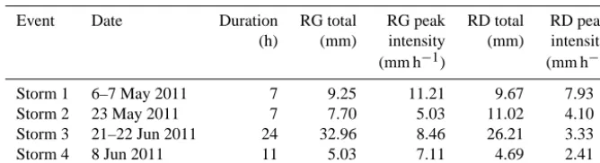
Table 1. Selected rainfall events over the Portobello catchment.

Event Date Duration RG total RG peak RD total RD peak (h) (mm) intensity (mm) intensity (mm h−1) (mm h−1)

Storm 1 6–7 May 2011 7 9.25 11.21 9.67 7.93

Storm 2 23 May 2011 7 7.70 5.03 11.02 4.10

Storm 3 21–22 Jun 2011 24 32.96 8.46 26.21 3.33

Storm 4 8 Jun 2011 11 5.03 7.11 4.69 2.41

Note: the accumulation and peak intensity values shown in this table correspond to areal mean values for the entire domain under consideration (as shown in Fig. 3b).

these parameters, the runoff volume at each sub-catchment is estimated using the NewUK rainfall–runoff model (Os-borne, 2001). The estimated runoff is then routed to the sub-catchment outlet using the Wallingford (double linear reser-voir) model (HR Wallingford, 1983). Sewers are modelled as one-dimensional conduits and flows within them are sim-ulated based on the full de Saint-Venant equations (i.e. fully hydrodynamic model).

The Portobello model contains a total of 1116 sub-catchments, with areas ranging between 0.02 and 24.42 ha and a mean area of 2.3 ha. Sub-catchment slopes range from 0.0 to 0.63 m m−1_{, with a mean slope of 0.031 m m}−1_. The model of the sewer system comprises 2917 nodes and 2907 conduits, in addition to 14 pumps. The total length of modelled sewers is 250 km. The sewer system ranges in height from 186.6 mAOD at Comiston to 3.8 mAOD along the Firth of Forth. 2 % of the modelled pipes have a gradient between 0.1 and 0.25 m m−1, 55 % have a gradient between 0.01 and 0.1 m m−1, and 43 % have a gradient<0.01 m m−1. Following UK standards (WaPUG, 2002) and using solely rain gauge data as input, the model of the Portobello catch-ment was manually calibrated in 2011 based upon three storm events recorded during the medium-term flow sur-vey described below. For the three storm events used for model calibration, the following mean performance statis-tics were obtained: Nash–Sutcliffe efficiency of 0.5782, root mean square error of 0.0373 m3s−1, coefficient of determi-nation (R2) of 0.7756 and regression coefficient (β), which provides a measurement of conditional bias, of 0.8826. 3.1.2 Local monitoring data (medium term survey) Local rainfall and flow data were collected in the Porto-bello catchment through a medium-term flow survey carried out between April and June 2011. The survey comprised 12 tipping bucket rain gauges and 28 flow monitoring sta-tions (each comprising a depth and a velocity sensor, based upon which flow rates were estimated). Both rain gauge and flow records were available at a temporal resolution of 2 min. However, rain gauge records were linearly interpolated to 5 min, in order to ensure agreement with the temporal resolu-tion at which radar estimates were available (see Sect. 3.1.3).

The location of the local flow and rain gauges is shown in Fig. 3b.

3.1.3 Radar rainfall data

The Portobello catchment is within the coverage of C-band radars operated by the UK Met Office (Fig. 3b). Radar rain-fall estimates for the same period as the local flow survey (i.e. April–June 2011) were obtained through the British At-mospheric Data Centre (BADC). These estimates were avail-able at spatial and temporal resolutions of 1 km and 5 min, respectively, and correspond to a quality controlled multi-radar composite product generated with the UK Met Office Nimrod system (Golding, 1998), which incorporates correc-tions for the different errors inherent to radar rainfall mea-surements, including identification and removal of anoma-lous propagation (e.g. beam blockage and clutter interfer-ence), attenuation correction and vertical profile correction (for a full description of the Nimrod system, the reader may refer to Harrison et al. (2000, 2009)).

3.1.4 Storm events selected for analysis

During the monitoring period (April–June 2011), four rel-evant storm events were captured which comply with UK standards for calibration and verification of urban drainage models (i.e. these events have instantaneous rainfall rates>5 mm h−1and accumulation>5 mm) (Gooch, 2009). Three of these events (referred to as Storms 1, 2 and 3) were used for calibration of the urban drainage model of the Por-tobello catchment (following UK standards, as mentioned above). In this study, all four storm events, including one not used in the calibration of the model (Storm 4), were used to test the proposed singularity-sensitive merging method. The dates and main statistics of the four selected events are sum-marised in Table 1. It is worth mentioning that, given the response time of the catchment, as well as inter-event time definition thresholds (IETD) recommended in the literature (Guo and Adams, 1998), a minimum IETD of 6 h was used as criteria to differentiate rainfall events.

du-ration. Moreover, well-structured storm cell clusters crossing the catchment area can be found in Storms 1, 3 and 4, but not in Storm 2. This is reflected in the lower RG peak intensity observed in Storm 2.

3.2 Evaluation methodology

The performance of the proposed singularity-sensitive Bayesian method (SIN hereafter) is assessed by inter-comparison against radar (RD), rain gauge (RG) and block-kriged (BK) interpolated RG estimates, as well against adjusted estimates resulting from the original Bayesian (non singularity-sensitive) technique (BAY) and the com-monly used mean field bias (MFB) adjustment method. It is important to note that, in this work, the MFB was implemented in a relatively dynamic way by comput-ing a sample cumulative bias (Bt) at each time step as

Bt=PRGcatchment/PRDco-located, where RGcatchment and RDco-locatedrepresent the rain gauge and the co-located radar grid rainfall estimates over the experimental catchment dur-ing the last hour. The MFB adjusted estimates are obtained by multiplying the bias (Bt) at each particular time step by

the original rainfall field; that is, MFB=Bt·RD.

Two evaluation strategies were applied:

1. Through analysis of the different rainfall estimates, us-ing as main reference local rain gauge records, while also inter-comparing the behaviour of other estimates. 2. Through analysis of the hydraulic outputs obtained by

feeding the different rainfall estimates as input to the hy-draulic model of the Portobello catchment and compar-ison of these with available flow records. Note that the RG estimates were applied to the model using Thiessen polygons.

Both evaluation strategies have inherent limitations which are next described. However, they provide useful and com-plementary insights into the performance of the proposed merging method.

The first strategy is a natural and widespread way of as-sessing the performance of rainfall products. However, the fact that all precipitation estimates entail errors and that the true rainfall field is unknown, in addition to the differences in the spatial and temporal resolutions of RG and RD esti-mates (and the resulting merged rainfall products), renders any direct comparison of rainfall estimates imperfect (Bran-des et al., 2001). In the particular case of rain gauge records, which are used as main reference in the present investiga-tion, errors can arise from a variety of sources (Einfalt and Michaelides, 2008). In order of general importance, system-atic errors common to all rain gauges include errors due to wind field deformation above the gauge orifice, errors due to wetting loss in the internal walls of the collector, errors due to evaporation from the container, and errors due to in-and out-splashing of water. In addition, tipping bucket rain

gauges, such as the ones used in this investigation, are known to underestimate rainfall at higher intensities because of the rainwater amount that is lost during the tipping movement of the bucket (La Barbera et al., 2002). This is a systematic er-ror unique to the tipping bucket rain gauge and is of the same order of importance as wind-induced losses. Besides these systematic errors, tipping bucket rain gauge records are also subject to local random errors, mainly related to their discrete sampling mechanism (Ciach, 2003; Habib et al., 2008). The order of magnitude of the two main error sources associated with tipping bucket rain gauges is 2–10 % for wind-induced losses (depending on wind speed, weight of precipitation and gauge construction parameters) (Sevruk and Nešpor, 1998) and up to 10 % for rainfall intensities of 100 mm h−1 and 20 % for intensities of 200 mm h−1, for water losses dur-ing the tippdur-ing action (Luyckx and Berlamont, 2001; Molini et al., 2005). Given that the storm events under investigation were not extremely heavy and that a basic quality-control was applied to ensure the quality of rain gauge measurements (e.g. manual comparison between neighbouring rain gauge data), the rain gauge records used in this study can be deemed acceptable as reference for the evaluation of other rainfall products. However, they are not perfect and the reader must keep in mind that the true rainfall field remains unknown.

The second strategy (i.e. hydraulic evaluation) allows some of the limitations of the rainfall evaluation strategy to be overcome, and is particularly useful when dense flow records are available, as is the case in the Portobello catch-ment. However, it has two main deficiencies: the fact that flow records (obtained based upon depth and velocity mea-surements) used in the evaluation contain errors, and the fact that the hydraulic modelling results encompass uncertainties from different sources in addition to rainfall input uncertainty (Deletic, 2012; Kavetski et al., 2006). In this regard, it is worth reminding the reader that the hydraulic model used in this study was calibrated using as input RG data. In fact, the model was calibrated based upon the data of Storms 1–3, which are used for testing in the present paper (Storm 4 is the only event not used in the calibration of the model). Since the model was “attuned” for RG inputs, it favours all RG-derived (and RG-emulating) rainfall estimates. Moreover, the rela-tively coarse spatial resolution of rainfall inputs (in this case

3.2.1 Methodology for analysis of rainfall estimates The performance of the SIN rainfall products in relation to other rainfall estimates (including RD, RG, BAY and MFB) is evaluated in terms of accumulations and rainfall rates at the areal level (i.e. at a scale corresponding to the area over which the Portobello catchment stretches) and at individual point gauge locations. In addition, a qualitative assessment of the spatial structure of the different (gridded) rainfall prod-ucts is carried out based upon visual inspection of images of the rainfall fields at the time of areal average peak intensity.

In view of the high density and coverage of the RG net-work over the Portobello catchment, the areal average RG estimates in the areal level analysis are assumed to be a good approximation of the “true” areal (average) rainfall over the experimental catchment (i.e. the areal reduction effect is ex-pected to be minor – Bell, 1976) and are therefore used as reference to evaluate the performance of the different areal gridded rainfall estimates. The areal analysis includes com-parison of event areal average accumulations and peak in-tensities, as well as comparison of intensities throughout the duration of each event (through scatterplots using RG areal average intensities as reference).

In the analysis of rainfall estimates at rain gauge point lo-cations a cross-validation strategy was adopted and three per-formance statistics are used. The cross-validation strategy, also referred to as “leave-one-out”, is an iterative method in which, at each iteration, data from one RG site is omitted from the calculations and the value at the “hidden” (i.e. omit-ted) location is estimated using the remaining data. Perfor-mance statistics are then computed from the comparison be-tween the estimated and the known (but not used) values (Velasco-Forero et al., 2009). The following three perfor-mance statistics are used in the present study. Firstly, a sam-ple bias ratio (B) is used to quantify the cumulative bias be-tween gridded rainfall estimates (i.e. RD, BK, MFB, BAY and SIN) and RG estimates at each RG location over the event period under consideration. B=1 means no cumu-lative bias between the RG and the given gridded rainfall estimates (i.e. equal rainfall accumulation recorded by RG and the gridded product at the given gauge location);B >1 means that the accumulations of the gridded estimates at the point locations are greater than those recorded by RG, and B <1 means the opposite. In addition to the comparison of rainfall accumulations, a simple linear regression analysis is applied to each pair of “instantaneous” (rain rate) point RG records and the co-located gridded estimates. The re-sults of the regression analysis are presented in terms ofR2 (coefficient of determination) andβ (regression coefficient, i.e. the slope or gradient of the linear regression). These two measures provide an indication of how well RG rates are replicated by the different rainfall estimates at each gaug-ing location, both in terms of pattern and accuracy. TheR2 measure ranges from 0 to 1 and describes how much of the “observed” (RG) variability is explained by the

“mod-elled” (RD/BK/adjusted) one. In practical terms,R2provides a measurement of the similarity between the patterns of the observed (i.e. RG) and “modelled” (i.e. gridded estimates) rainfall time series at a given gauging location. However, sys-tematic bias (under- or over-estimation) of the modelled es-timates cannot be detected from this measure (Krause et al., 2005). The regression coefficient,β, is therefore employed to provide this supplementary information to theR2.β≈1 represents good agreement in the magnitude of the rainfall rates recorded by RG and those of the gridded estimates; β >1 means that the rain rates associated with the gridded estimate are higher in the mean (by a factor ofβ) than those recorded by RG; andβ <1 means the opposite (i.e. rain rates of gridded estimates are lower in the mean than RG ones). 3.2.2 Methodology for analysis of hydraulic outputs A qualitative analysis of the hydraulic outputs is carried out based upon visual inspection of recorded vs. simulated flow hydrographs (for the different rainfall inputs) at different points of the catchment. Furthermore, similar to the rain-fall analysis, a simple linear regression analysis is applied to each pair of recorded and simulated flow time series (at each flow gauging location). The performance of the asso-ciated hydraulic simulations is evaluated using theR2 and β statistics obtained from the linear regression analysis. In addition, the “weighted” coefficient of determination (R2_w) is employed to quantify the joint performance of hydrological efficiency. This measure is defined as (Krause et al., 2005) R_w2=

|β| ·R2 forβ≤1

|β|−1·R2 forβ >1, (8) where higherR_w2 values correspond to better hydraulic per-formance.

Table 2. Areal average rainfall accumulations and peak intensities

for the different rainfall products.

Input Storm 1 Storm 2 Storm 3 Storm 4

AVG rainfall RG 9.25 7.70 32.96 5.03

accumulation RD 9.80 11.02 26.21 4.69

(mm) BK 8.87 7.77 31.41 4.08

MFB 8.64 7.25 31.87 4.55

BAY 8.76 7.79 27.24 3.81

SIN1 9.37 7.95 33.37 4.82

SIN2 9.37 7.95 33.38 4.83

SIN3 9.38 7.95 34.43 4.85

SIN4 9.41 7.96 33.73 4.94

SIN5 9.61 8.04 31.57 5.23

AVG rainfall peak RG 11.21 5.03 8.46 7.11 intensity over 5 min RD 7.93 4.10 3.33 2.41

(mm h−1) BK 10.66 4.54 7.59 5.09

MFB 9.06 4.68 4.05 3.34

BAY 10.47 3.80 6.82 4.92

SIN1 13.17 5.08 8.00 6.97

SIN2 13.17 5.08 8.00 6.97

SIN3 13.17 5.08 8.00 6.98

SIN4 13.19 5.08 8.01 7.03

SIN5 13.53 5.09 8.27 7.25

and recommendations from studies focusing on the perfor-mance of flow gauges; Marshall and McIntyre, 2008). 3.3 Results and discussion

3.3.1 Rainfall estimates Areal rainfall estimates

Table 2 shows the areal average (AVG) accumulations and peak intensities for the different rainfall products for the four storm events under consideration. As can be seen, the differ-ence between RD and RG event areal average accumulations is generally small, yet it is event-varying. For Storms 1 and 2, the areal average RG totals are slightly overestimated by the RD estimates, while for Storms 3 and 4 they are underesti-mated, with the underestimation being largest in Storm 3. In terms of areal average peak intensities, RD estimates appear to consistently underestimate the areal average peak intensi-ties recorded by RG. The relative difference between RG and RD areal average peak intensities is approximately 20–30 % for Storms 1 and 2, and it is as high as 60 % for Storms 3 and 4. This indicates that the RD estimates could not satisfac-torily capture instantaneous rainfall rates, particularly high rainfall rate values, and corroborates the need for dynamic adjustment of RD estimates using local RG measurements.

As would be expected, the BK estimates exhibit areal av-erage accumulations and peak intensities similar to those of the RG. Small differences are observed (in general BK val-ues are slightly lower than RG ones) which can be generally attributed to the area-point rainfall differences (Anagnostou and Krajewski, 1999). These differences become more

evi-Figure 4. Histogram of singularity exponents (α) at the time of areal peak intensity for the four selected storm events.

dent when analysing results at individual gauge locations (in next section).

When looking at the adjusted rainfall products (i.e. MFB, BAY and SIN), it can be seen that all of them can improve the original RD estimates, but the degree of improvement is different for each method. As expected, the MFB success-fully reduces the difference in event areal average accumula-tions (i.e. bias), leading to areal average accumulaaccumula-tions close to those recorded by RG. In terms of peak intensities, the MFB method leads to some improvement, but the resulting peak intensities are still significantly lower than the RG ones. Although the MFB was applied dynamically with an hourly frequency of bias correction, these results suggest that more dynamic and spatially varying (higher order) methods than the MFB are required in order to successfully adjust radar rainfall estimates for urban hydrological applications.

Figure 5. Scatterplots of instantaneous areal average RG vs. RD/BK/MFB/BAY/SIN rainfall rates over the Portobello catchment for the four

selected events, where SIN1–SIN5 represent the SIN estimates with different “truncated” singularity ranges (from widest to narrowest).

(from SIN1 to SIN5), the areal accumulations and peak in-tensities tend to be higher. A particular steep increment is observed in the areal accumulations and peak intensities of SIN5, in relation to the other singularity ranges, which re-sults in a slight overestimation of accumulations and peak intensities, as compared to the RG estimates. This is espe-cially apparent in Storms 3 and 4. The increment in rainfall accumulation and peak intensities as the singularity range becomes narrower can be explained by the fact that at nar-rower ranges, only part of the singularity structures are re-moved before merging, and a big proportion of them remains in the radar image. This is evident from Fig. 4, where it can be seen that for Storms 3 and 4 a significant number of sin-gularity exponents spread beyond the narrowest sinsin-gularity range (i.e. SIN5: α∈[1.75, 2.25]). The problem arises cause some singularity features remain in the radar image be-fore the BAY merging is applied, and these may be partially preserved throughout the merging process. Afterwards, when the extracted singularity component is applied back and pro-portionally to the merged rainfall field, it may interact (in a nonlinear fashion) with the singularity structures preserved throughout the BAY merging, thus leading to an

overestima-tion of extremes (whether these are enrichments or deple-tions). These results suggest that a better approach is to be sure to remove most of the singularity structures before car-rying out the merging. Therefore, very narrow ranges such as SIN5 should be avoided. In fact, it can be seen that the in-termediate range of SIN3 (i.e.α∈[1, 3]) covers most singu-larity exponents (see Fig. 4). Indeed, using wider singusingu-larity ranges leads to very similar results as those obtained when using the SIN3 range (notice the similarity between SIN1, SIN2 and SIN3 estimates in Table 2). This suggests that the singularity range of [1, 3] is appropriate.

peak intensities, with underestimation being more evident in the events with relatively high intensities (i.e. Storms 1, 3 and 4). Unlike BK estimates, the difference between areal RD and RG peak intensities is too large to be entirely ex-plained by areal-point differences. The fact that the RD esti-mates display relatively good performance in (long-duration) accumulations but not in (short-duration) instantaneous in-tensities corroborates the claim that RD estimates fail to cap-ture the short-term dynamics of small-scale rainfall. As men-tioned in Sect. 1, the main reason for this lies in the use of a staticZ–Rconversion function, which represents a statisti-cal compromise for the range of rainfall rates that frequently occur (whereas the occurrence of very small and large in-tensities is relatively rare). Concerning the MFB method, from Fig. 5 it can be seen that it fails to satisfactorily im-prove RD instantaneous rainfall rates; this is particularly ev-ident at high intensities, at which, similarly to RD estimates, MFB estimates perform poorly. An accurate representation of peak intensities is of outmost importance in the modelling and forecasting of urban pluvial flooding. This confirms that, being a first-order technique, the MFB adjustment method may be insufficient for urban-scale applications. In contrast, it can be seen that over- and underestimation errors in RD estimates can be improved by second- or higher-order ad-justment techniques, such as BAY and SIN. In fact, in terms of instantaneous rainfall rates the BAY estimates display a significantly better performance than the MFB ones. How-ever, the BAY estimates still fail to properly reproduce the highest intensities. These shortcomings of the BAY method seem to be overcome by the incorporation of the singularity analysis: indeed, the SIN estimates exhibit the best overall performance, particularly at peak intensities. In agreement with the results displayed in Table 2, in Fig. 5 it can be seen that as the singularity range becomes narrower, rainfall es-timates with slightly higher intensities are generated. More-over, it can be noticed that wider singularity ranges lead to more conservative results and appear to be a good choice. Rainfall estimates at gauging locations

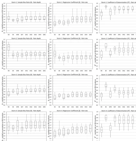
The aforementioned features of the different rainfall esti-mates are further highlighted through analysis at each rain gauge location; the associated statistics, including sample bias (B), regression coefficient (β) and coefficient of deter-mination (R2), are summarised in Fig. 6.

As expected, the RD estimates (before adjustment) display the largest differences from point RG estimates: in general, they possess the largest cumulative bias (B) and the low-estR2, and their statistics show great variability. Moreover, the distribution of the β values indicates that RD estimates tend to largely underestimate RG instantaneous rainfall rates. This is the case for all storm events, except for Storm 2, for which rainfall intensities were low on average.

Similarly to the results of the areal (average) analysis, the individual-site BK estimates display the closest behaviour to

the RG ones. This is of course expected given that the BK estimates are obtained by simple interpolation of point RG data. It can be seen that the BK estimates are nearly unbi-ased (Bis very close to 1) and possess the highestR2 medi-ans (i.e. closest to 1), as well as the narrowestR2boxes and whiskers. However, when looking at the distribution ofβ val-ues of the BK estimates, it can be seen that most of the time the whole boxes and whiskers are below 1. This reflects a systematic underestimation of rainfall rates at point gauging locations, which is discussed below.

With regard to the adjusted rainfall estimates, the MFB method is found to bring original radar estimates slightly closer to RG ones, but the improvement seems insufficient. As expected, the main improvement of MFB estimates is found in the bias (B), which is significantly reduced (thus be-coming closer to 1). In terms of instantaneous rainfall rates, the improvement provided by MFB is very limited. This is re-flected in the lowR2values and in the poorβscores, which remain remarkably close to those of the original RD esti-mates. Similar to the results of the areal analysis, these re-sults suggest that the MFB adjustment method is insufficient for urban-scale applications, in which small-scale rainfall dy-namics are critical.

When looking at the statistics of the BAY estimates, it can be noticed that these behave similarly to the BK ones: their bias is also small, theR2is generally high and theβ values are systematically below 1. The similarity in the behaviour of BK and BAY estimates suggests that for the selected events, the BAY method tends to trust the (smooth interpolated) BK estimates more than the RD estimates. As explained in Sects. 1 and 2, this is the main shortcoming of the BAY method. The systematic underestimation of rainfall rates ob-served in BK and BAY estimates (reflected byβvalues sys-tematically below 1) can be partially explained by the areal reduction effect. However, considering that the individual-site comparison was conducted using instantaneous rainfall estimates for very short time intervals (i.e. 5 min), one would expect the tendency of the areal-point differences to be of higher randomness, rather than of a systematic nature. This suggests that the systematic underestimation may be a joint consequence of the areal reduction effect and of the under-lying second-order approximation (which smooths off some local extreme magnitudes).

re-Figure 6. Boxplots displaying the distribution of sample bias ratio (B) (left column panels), regression coefficient (β) (middle column panels) and coefficient of determination (R2) (right column panels) estimated between the different gridded rainfall estimates and RG records at individual rain gauge locations following a cross-validation approach.

sults of the areal analysis, this serves to further highlight two important features of the proposed SIN method: it generally respects the commonly observed areal reduction effect, and it integrates more small-scale randomness from RD data in the data-merging process. Regarding the singularity ranges, a similar behaviour can be observed for all of them, although a slight tendency can be observed for the bias (B) andβ val-ues to increase as the singularity range becomes narrower. This is in agreement with the results of the areal analysis and suggests that working with intermediate ranges, as opposed

to very narrow ones which can truncate the singular struc-tures, is advisable.

Spatial structure of rainfall fields

men-Figure 7. Snapshot images of the different spatial rainfall products at the time of peak areal intensity for Storms 1 (top panels) to 4 (bottom

panels) over the Portobello catchment. From left to right panels: RD, BK, MFB, BAY and SIN3 (with singularity range [1, 3]) estimates. The black polygon indicates the boundary of the Portobello catchment, and the black and white markers respectively represent the location of flow and rain gauges.

tioned in the previous sections, the SIN3 range covers most of the singularity indices and consistently led to good results for the storms under consideration.

It can be seen that the spatial structure of the BK rainfall field (fully based upon rain gauge data) is highly symmet-ric and smooth, and is rather unrealistic. With regard to the adjusted rainfall products (MFB, BAY and SIN), it can be noticed that the proportion of radar (RD) and BK interpo-lated rain gauge features that are preserved varies accord-ing to the method. The MFB fields fully inherit the spatial structure of the RD fields; the only change is that the ac-tual intensity values are scaled up or down by an areal ratio derived from the sample bias between mean rain gauge and

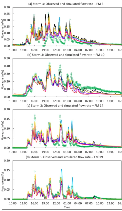
Figure 8. Observed flows vs. simulated flows with RG, RD, BK,

BAY and SIN3 rainfall inputs at selected flow gauging sites of Por-tobello catchment during Storm 3. Selected gauging sites: FM3: up-stream end of the catchment (top panels); FM10: mid-up-stream area (bottom panels). The location of the selected monitoring sites is shown in Fig. 3.

middle-left area of the BAY image of Storm 3 (see Fig. 7, top). However, these features appear to be much smoother and spreading over a larger area, as compared to their struc-ture in the original RD image. As compared to the BAY peak rainfall fields, the SIN fields display less smooth and more realistic structures which preserve more features of the orig-inal RD fields. In general, the inspection of the snapshot im-ages of the different rainfall products confirms the findings of the areal and point gauge analyses regarding the ability of the SIN method to better preserve the singularity structures present in rainfall fields (and captured by RD) throughout the merging process, as compared to the original BAY merging method.

Figure 9. Observed flows vs. simulated flows with SIN1–SIN5

rain-fall inputs at selected flow gauging sites of Portobello catchment during Storm 3. Selected gauging sites: FM14: upstream end of a small branch of the sewer system (top panels); FM19: downstream end of the catchment (bottom panels). The location of the selected monitoring sites is shown in Fig. 3.

3.3.2 Hydraulic modelling results

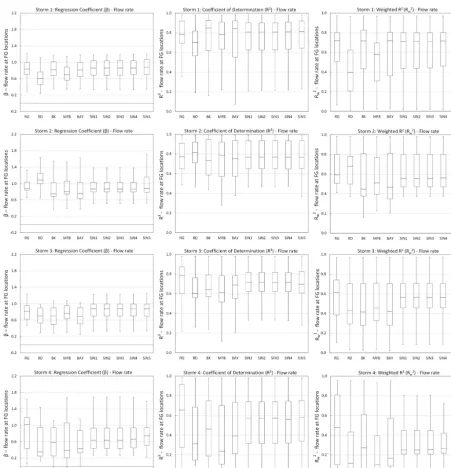
Figures 8 and 9 shows example observed vs. simulated flow hydrographs for the different rainfall inputs at four gauging locations (see locations in Fig. 3) during Storm 3. Note that Storm 3 is an event with high rainfall accumulations, rainfall rates and strong singularity structures. Figure 10 summarises the performance statistics resulting from the simple linear re-gression analysis (i.e.β,R2andR_w2) conducted at each flow gauging station for each storm event.

Figure 10. Boxplots displaying the distribution of regression coefficient (β) (left column panels), coefficient of determination (R2) (middle column panels) and weighted coefficient of determination (R2_w) (right column panels) statistics derived from the linear regression analysis conducted for each pair of recorded and simulated flow time series at each gauging location.

agreement with observations. This indicates that all rainfall products, including the RD before adjustment, can well cap-ture the general dynamics of rainfall fields. The main differ-ence between the simulated flows lies in their ability to re-produce flow peaks, which in turn is a function of the ability of the different rainfall estimates to reproduce peak rainfall rates in terms of magnitude, timing and spatial distribution. In line with the results of the rainfall analysis, the flow hy-drographs associated with BK estimates are close to the ones associated with RG records; however, the former display a

by the statistics in Fig. 10 and corroborates the claim that the application of a “blanket” MFB correction over the area of interest is insufficient for urban applications. The BAY out-puts, on the other hand, show a consistent improvement over the RD outputs. Nonetheless, in agreement with the results of the rainfall analysis, the BAY estimates behave similarly to the BK ones and lead to smooth flow peaks which of-ten underestimate observations. The SIN outputs also show a consistent improvement over RD estimates, but, unlike BAY outputs, the SIN outputs do not smooth off flow peaks and instead show a better ability to reproduce these, sometimes leading to a better match of observed flow peaks than RG as-sociated outputs (which were used as input for the calibration of the model). With regard to the singularity ranges, it can be seen that the differences observed in the SIN1–SIN5 rainfall estimates are mostly filtered out when converting rainfall to runoff. As a result, the flow outputs of all SIN estimates are very similar and their hydrographs can barely be differenti-ated.

The preliminary conclusions drawn from the visual in-spection of the selected hydrographs are corroborated by the statistics in Fig. 10. As would be expected, the RG outputs generally show the best performance in all statistics (except for Storm 2). It is nonetheless noteworthy that theβ values for RG estimates (for which the model was calibrated) are generally below 1. This reveals a slight bias of the model to underestimate flows and partially explains the fact thatβ val-ues associated with all rainfall inputs are mostly below 1. With regard to the BK (i.e. interpolated RG) associated out-puts, the tendency to underestimate, which is observed in the rainfall analysis, becomes even more evident in the hydraulic outputs: BK’s β values are significantly lower than 1 and lower than the β values associated with RG estimates. Dif-ferent from the results of the rainfall analysis, in which those products closest to RG estimates (including BK) displayed the best performance in terms ofR2, in the hydraulic analy-sis BK outputs generally lead to a deterioration inR2values (see statistics of Storms 2, 3 and 4). This suggests that the smoothing caused in the BK interpolation affects the small-scale dynamics of rainfall fields, leading to poor representa-tion of associated flow dynamics. Contrary to RG-associated outputs, RD flow estimates generally display the worst per-formance. In agreement with the results of the rainfall anal-ysis, RD outputs show a tendency to largely underestimate flows (as indicated by β values well below one and much lower than those obtained for RG outputs). Moreover, they display relatively lowR2and associatedR_w2values. Nonethe-less, a special case is observed in Storm 2, when RD esti-mates, which in the rainfall analysis displayed the poorest performance, yielded the best flow simulations, thus empha-sising the added value that RD estimates can provide, as well as the complementary information provided by the hydraulic evaluation strategy. In the cases in which RD outputs per-form poorly (i.e. in Storms 1, 3 and 4), all adjusted rainfall estimates lead to improvements over RD hydraulic results,

with the degree of improvement varying according to the ad-justment technique. In Storm 2, when RD outputs displayed the best performance, the different merging methods showed to retain different degrees of RD features. Overall, it can be seen that the MFB estimates provide little improvement over the original RD estimates. In the cases in which RD led to systematic underestimation of flows, the MFB estimates managed to slightly reduce this underestimation by bringing βvalues closer to 1, as compared to those of the original RD estimates. However, in Storm 2, in which RD outputs per-formed best, MFB caused a large deterioration ofβ values, whereas the SIN estimates managed to keepβ scores closer to 1. In terms ofR2, the MFB estimates do not provide much improvement and can actually lead to a deterioration of this statistic (e.g. Storms 2 and 4), suggesting that the applica-tion of the MFB adjustment can alter the spatial-temporal structure of the original RD fields. The BAY outputs show a greater improvement than MFB, particularly in terms ofR2. Nonetheless, in agreement with the rainfall analysis and with the visual inspection of hydrographs, the BAY outputs be-have remarkably similarly to BK ones. One of the main fea-tures of the BAY outputs is that they lead to systematically lower flows than RG estimates (noteβ values consistently lower than those of RG outputs). This confirms the smooth-ing of rainfall peaks that occurs when second-order approx-imations are applied. Lastly, it can be seen that the SIN puts display the greatest improvement over original RD out-puts, both in terms of correcting systematic bias, as well as in terms of well reproducing rainfall and associated flow pat-terns. As compared to MFB and BAY outputs, the SIN out-puts generally displayβvalues closer to 1, higherR2values (sometimes even higher than those of RG outputs) and con-sequently higherR2_wvalues. The better performance of SIN hydraulic outputs over BAY ones, particularly in terms ofβ, provides an a posteriori confirmation that it was right, in the SIN method, to view the singularities in the radar field as ac-tual features of the real rainfall. Similarly as was observed in the hydrographs in Figs. 8 and 9, the performance of the dif-ferent SIN ranges is very similar. In line with the results of the rainfall analysis, SIN5 shows a slight tendency towards higher flows, which sometimes resulted in better hydraulic statistics. Nonetheless, the differences are small and, based upon the findings of the rainfall analysis, the adoption of a wider SIN range and removal of most singularities appears to be a more conservative option. However, this aspect must be further investigated using a wider range of storm events and pilot catchments.

of the hydraulic outputs associated with the different rain-fall inputs was generally consistent in all storm events under consideration. The particular differences that were observed were due to the nature of a given storm and not to the fact that a given event was used for model calibration or not.

4 Conclusions and future work

In this paper, a new gauge-based radar rainfall adjustment method was proposed, which aims at better merging rainfall estimates obtained from rain gauges and radars, at the small spatial and temporal scales characteristic of urban catch-ments. The proposed method incorporates a local singularity analysis into the Bayesian merging technique (Cheng et al., 1994; Todini, 2001). Through this incorporation, the merging process preserves the fine-scale singularity (non-Gaussian) structures present in rainfall fields and captured by radar, which are often associated with local extremes and are gen-erally smoothed off by currently available radar–rain gauge merging techniques, mainly based upon Gaussian approxi-mations.

Using as case study four storm events observed in the Por-tobello catchment (53 km2) (Edinburgh, UK) in 2011, the performance of the proposed singularity-sensitive Bayesian data-merging (SIN) method, in terms of adjusted rainfall estimates and the subsequent runoff estimates, was eval-uated and compared against that of the original Bayesian data-merging (BAY) technique and the widely used mean field bias correction (MFB) method. This analysis clearly brought out the benefits of introducing the singularity-sensitive method. The results suggest that the proposed SIN method can effectively identify, extract and preserve the sin-gular structures present in radar images while retaining the accuracy of rain gauge (RG) estimates. This is reflected in the better ability of the SIN method to reproduce in-stantaneous rainfall rates, rainfall accumulations and associ-ated runoff flows. This method clearly outperforms the com-monly used MFB adjustment, which simply fails to repro-duce the dynamics of rainfall in urban areas, and the original BAY method, which shows an overall good performance but smooths off peak rainfall magnitudes, thus leading to under-estimation of runoff extremes.

In this study the sensitivity of the SIN results to the “de-gree” of singularity that is removed from the radar image and preserved throughout the merging process was also tested. While the impact of it was found to be generally small, the re-sults suggest that partially removing singularities could have a negative impact on the results. Therefore, removing most singularity exponents from the original radar image is advis-able.

While the proposed singularity method has shown great potential to improve the merging of radar and rain gauge data for urban hydrological applications, further testing including more storm events and pilot catchments is still required in

or-der to ensure that the results are not case specific and to draw more robust conclusions about the applicability of the pro-posed method. Other aspects on which further work is rec-ommended are the following:

a. The current version of the singularity-sensitive method shows a slight tendency to overestimate rainfall rates and accumulations. This is likely to be due to one of two aspects, or a combination of them:

– In the eventual case in which a rain gauge is lo-cated within the core of a convective cell, the re-sulting interpolated (block-kriged; BK) field may end up having singularity structures and, as ex-plained in Sect. 2.3, this may ultimately lead to “double-counting” of singularities. For the time be-ing, a moving-window smoothing has been applied on the BK field before it is merged with the non-singular radar field, so as to remove non-singularity structures potentially present in the BK field. While this has proven to be an acceptable solution, we believe it can be further refined. Other methods for dealing with this particular problem have been tested, including extraction of singularities from the point rain gauge records using the singularity ex-ponents derived from the co-located radar pixels, and extraction of singularities from the BK field us-ing local sus-ingularity analysis. However, these have proven unstable and highly uncertain. Further work to better deal with this issue is required.

– The asymmetric distribution of singularity expo-nents and the numerical stability of singularity ex-traction from a small set of data samples. This drawback could be improved by forcing the mean of non-singular components to remain equal to the original radar estimates (Agterberg, 2012a). Alter-natively, other techniques for singularity identifi-cation and extraction could be used. For example, the wavelet transformation (Kumar and Foufoula-Georgiou, 1993; Mallat and Hwang, 1992; Robert-son et al., 2003; Struzik, 1999), Principal Com-ponent Analysis (Gonzalez-Audicana et al., 2004; Zheng et al., 2007) and Empirical Mode Decom-position (Nunes et al., 2003, 2005) techniques are widely recommended in the literature.

b. Given that the proposed singularity-sensitive merging method is particularly intended to improve rainfall es-timates for (small-scale) urban areas, it would be inter-esting to test it using higher spatial-temporal resolution data (e.g. from X-band radars).

method) is conducted. However, doing this would somehow miss the point of the proposed method. The key point here is that for a non-Gaussian structure, moments beyond the second order are important, as each brings new information worth preserving. To create a more “normal” field is not the purpose of the singularity extraction; instead, it is the conse-quence after removing singularities from the rainfall fields, which can be physically associated with abnormal energy concentration, such as “convective” cells, and which in the proposed method are set aside to ensure their preservation throughout the merging process.

The Supplement related to this article is available online at doi:10.5194/hess-19-4001-2015-supplement.

Acknowledgements. The authors would like to acknowledge

the support of the Interreg IVB NWE RainGain project, the Research Foundation-Flanders (FWO) and the PLURISK project for the Belgian Science Policy Office of which this research is part. Special thanks go to Alex Grist and Richard Allitt, from Richard Allitt Associates, for providing the rain gauge data and the hydraulic model, and for their constant support with the hydraulic simulations. Thanks are also due to the UK Met Office and the BADC (British Atmospheric Data Centre) for providing Nimrod (radar) data, to Innovyze for providing the InfoWorks CS software, and to Cinzia Mazzetti and Ezio Todini for making freely available to us the RAINMUSIC software package for meteorological data processing. Lastly, the authors would like to thank the reviewers, Scott Sinclair and Cinzia Mazzetti, and the Editor, Uwe Ehret, for their insightful and constructive comments which helped improved the manuscript significantly.

Edited by: U. Ehret

References

Agterberg, F. P.: Mixtures of multiplicative cascade models in geochemistry, Nonlin. Processes Geophys., 14, 201–209, doi:10.5194/npg-14-201-2007, 2007.

Agterberg, F. P.: Multifractals and geostatistics, J. Geochem. Ex-plor., 122, 113–122, doi:10.1016/j.gexplo.2012.04.001, 2012a. Agterberg, F. P.: Sampling and analysis of chemical element

con-centration distribution in rock units and orebodies, Nonlin. Processes Geophys., 19, 23–44, doi:10.5194/npg-19-23-2012, 2012b.

Anagnostou, E. N. and Krajewski, W. F.: Real-time radar rainfall es-timation, Part I: Algorithm formulation, J. Atmos. Ocean. Tech., 16, 189–197, 1999.

Bell, F. C.: The Areal Reduction Factor in Rainfall Frequency Es-timation, Centre for Ecology & Hydrology (CEH), Wallingford, 1976.

Bowler, N. E., Pierce, C. E., and Seed, A. W.: STEPS: a probabilistic precipitation forecasting scheme which merges an extrapolation

nowcast with downscaled NWP, Q. J. Roy Meteorol. Soc., 132, 2127–2155, doi:10.1256/qj.04.100, 2006.

Brandes, E. A., Ryzhkov, A. V and Zrni´c, D. S.: An eval-uation of radar rainfall estimates from specific differential phase, J. Atmos. Ocean. Tech., 18, 363–375, doi:10.1175/1520-0426(2001)018<0363:AEORRE>2.0.CO;2, 2001.

Chen, Z., Cheng, Q., Chen, J., and Xie, S.: A novel iterative ap-proach for mapping local singularities from geochemical data, Nonlin. Processes Geophys., 14, 317–324, doi:10.5194/npg-14-317-2007, 2007.

Cheng, Q.: Multifractality and spatial statistics, Comput. Geosci., 25, 949–961, doi:10.1016/S0098-3004(99)00060-6, 1999. Cheng, Q. and Zhao, P.: Singularity theories and methods

for characterizing mineralization processes and mapping geo-anomalies for mineral deposit prediction, Geosci. Front., 2, 67– 79, doi:10.1016/j.gsf.2010.12.003, 2011.

Cheng, Q., Agterberg, F. P., and Ballantyne, S. B.: The sepa-ration of geochemical anomalies from background by fractal methods, J. Geochem. Explor., 51, 109–130, doi:10.1016/0375-6742(94)90013-2, 1994.

Ciach, G. J.: Local random errors in tipping-bucket rain gauge measurements, J. Atmos. Ocean. Tech., 20, 752– 759, doi:10.1175/1520-0426(2003)20<752:LREITB>2.0.CO;2, 2003.

Collier, C. G.: Accuracy of rainfall estimates by radar, part I: Cal-ibration by telemetering raingauges, J. Hydrol., 83, 207–223, doi:10.1016/0022-1694(86)90152-6, 1986.

Collier, C. G.: Applications of Weather Radar Systems, 2nd Edn., Wiley, Chichester, England, 1996.

Deletic, A., Dotto, C. B. S., McCarthy, D. T., Kleidorfer, M., Freni, G., Mannina, G., Uhl, M., Henrichs, M., Fletcher, T. D., Rauch, W., Bertrand-Krajewski, J. L., and Tait, S.: Assess-ing uncertainties in urban drainage models, Phys. Chem. Earth Pt. A/B/C, 42–44, 3–10, doi:10.1016/j.pce.2011.04.007, 2012. Einfalt, T. and Michaelides, S.: Quality control of precipitation data,

in: Precipitation: Advances in Measurement, Estimation and Pre-diction SE-5, edited by: Michaelides, S., Springer, Berlin, Hei-delberg, 101–126, 2008.

Einfalt, T., Arnbjerg-Nielsen, K., Golz, C., Jensen, N.-E., Quirm-bach, M., Vaes, G., and Vieux, B.: Towards a roadmap for use of radar rainfall data in urban drainage, J. Hydrol., 299, 186–202, doi:10.1016/j.jhydrol.2004.08.004, 2004.

Einfalt, T., Jessen, M., and Mehlig, B.: Comparison of radar and raingauge measurements during heavy rainfall, Water Sci. Tech-nol., 51, 195–201, 2005.

Evertsz, C. J. G. and Mandelbrot, B. B.: Multifractal measures, in: Chaos and Fractals, edited by: Peitgen, H.-O., Jurgens, H., and Saupe, D., Springer, New York, 922–953, 1992.

Fulton, R. A., Breidenbach, J. P., Dong-Jun, S., and Miller, D. A.: The WSR-88D rainfall algorithm, Weather Forecast., 13, 377–395, doi:10.1175/1520-0434(1998)013<0377:TWRA>2.0.CO;2, 1998.

Germann, U., Galli, G., Boscacci, M., and Bolliger, M.: Radar pre-cipitation measurement in a mountainous region, Q. J. Roy Me-teorol. Soc., 132, 1669–1692, doi:10.1256/qj.05.190, 2006. Gires, A., Onof, C., Maksimovi´c, C., Schertzer, D.,