The effect of flow and orography on the spatial distribution of the very short term predictability of rainfall from composite radar images

www.hydrol-earth-syst-sci.net/18/4671/2014/ doi:10.5194/hess-18-4671-2014

© Author(s) 2014. CC Attribution 3.0 License.

The effect of flow and orography on the spatial distribution

of the very short-term predictability of rainfall

from composite radar images

L. Foresti1,2,*and A. Seed2

1_{Royal Meteorological Institute of Belgium, Brussels, Belgium}

2_{Bureau of Meteorology, Centre for Australian Weather and Climate Research, Melbourne, Australia} *_{now at: Royal Meteorological Institute of Belgium, Brussels, Belgium}

Correspondence to: L. Foresti ([email protected])

Received: 27 June 2014 – Published in Hydrol. Earth Syst. Sci. Discuss.: 10 July 2014 Revised: 21 October 2014 – Accepted: 23 October 2014 – Published: 27 November 2014

Abstract. The spatial distribution and scale dependence of the very short-term predictability of precipitation by La-grangian persistence of composite radar images is studied under different flow regimes in connection with the presence of orographic features. Data from the weather radar compos-ite of eastern Victoria, Australia, a 500×500 km2domain at 10 min temporal and 2×2 km2spatial resolutions, covering the period from February 2011 to October 2012, were used for the analyses. The scale dependence of the predictability of precipitation is considered by decomposing the radar rain-fall field into an eight-level multiplicative cascade using a fast Fourier transform. The rate of temporal development of precipitation in Lagrangian coordinates is estimated at each level of the cascade under different flow regimes, which are stratified by applying a k-means clustering algorithm on the diagnosed velocity fields. The predictability of precipitation is measured by its lifetime, which is derived by integrating the Lagrangian auto-correlation function. The lifetimes were found to depend on the scale of the feature as a power law, which is known as dynamic scaling, and to vary as a function of flow regime. The lifetimes also exhibit significant spatial variability and are approximately a factor of 2 longer on the upwind compared with the downwind slopes of terrain fea-tures. The scaling exponent of the spatial power spectrum also shows interesting geographical differences. These find-ings provide opportunities to perform spatially inhomoge-neous stochastic simulations of space–time precipitation to account for the presence of orography, which may be inte-grated into design storm simulations and stochastic precipi-tation nowcasting systems.

1 Introduction

The scale dependence of the predictability of the atmospheric flow was already studied by Lorenz (1969), who found that there is an intrinsic predictability limit associated to each scale of motion. Similar conclusions can also be extended to the predictability of precipitation, in particular if considering rainfall fields as emerging from multiplicative cascade pro-cesses (Schertzer and Lovejoy, 1987; Marsan et al., 1996).

precipitation field into meaningful physical structures from the high to the low frequencies. Surcel et al. (2014) used a Discrete Cosine Transform to study the filtering properties of ensemble averaging and discovered that the ensemble mem-bers are completely decorrelated below a certain cutoff scale. The multifractal and scale-dependent nature of rainfall not only complicates the study of its predictability and the ver-ification of forecasts, but also demands more sophisticated forecasting and downscaling techniques. The Short-Term En-semble Prediction System (STEPS; Seed, 2003; Bowler et al., 2006) is a stochastic precipitation nowcasting scheme that exploits the multifractal principle by decomposing the radar rainfall field into an eight-level multiplicative cascade with an FFT. The cascade is advected with optical flow in Lagrangian coordinates and stochastically evolves in time according to a hierarchy of auto-regressive processes of or-der 1 – AR(1) – or 2 – AR(2). This allows accounting for the empirical observation that the rate of temporal evolution of precipitation features is a power law of the scale of the feature, which is known as dynamic scaling (see, e.g., Venu-gopal et al., 1999; Mandapaka et al., 2009). STEPS estimates the rate of Lagrangian development of the cascade levels in real time, which allows adapting to the predictability of the observed sequence of radar images. This is necessary since the predictability of precipitation exhibits a strong temporal variability as shown by Seed (2003), Germann et al. (2006), and Seed et al. (2013).

Germann et al. (2006) also analyzed the geographical dis-tribution of the predictability of precipitation over the con-terminous United States and found a region of longer life-times extending from eastern Nebraska to Lake Michigan through Iowa, Wisconsin, and northern Illinois. Berenguer and Sempere-Torres (2013) performed a similar analysis us-ing the European radar composite and discovered the pre-dictability to be seasonally dependent, with higher values over the central part of the UK, central continental Eu-rope, and the Baltic regions. However, such geographical dif-ferences are strongly affected by the inhomogeneous qual-ity of the European radar composite between the different countries, which use different hardware, operating wave-length, scanning strategy, and signal processing (Huusko-nen et al., 2014). The spatial heterogeneity of the statisti-cal properties of rainfall also poses issues for its multifractal simulation, which traditionally assumes spatial homogene-ity of the stochastic process. One way to avoid construct-ing complicated, spatially heterogeneous models is to sep-arately add a spatial trend to correct a homogeneous multi-fractal model. This trend should account for the spatial in-homogeneity of the long-term climatological distribution of precipitation, which is often controlled by the presence of orographic features (see, e.g., Pathirana and Herath, 2002; Badas et al., 2006).

The climatology of precipitation over complex orogra-phy is strongly controlled by flow direction and air stability (Panziera and Germann, 2010), which can also be exploited

to design analogue-based nowcasting techniques (Foresti et al., 2013). The contribution of orography to the precipitation enhancement also seems to be a scale-dependent process. This can be observed by extracting features from a digital elevation model (DEM) at different spatial scales and look-ing at the spatial distribution of persistent precipitation cells. It appears that orographic features need a certain character-istic size (scale) in order to control the spatial distribution of precipitation patterns (e.g., Foresti et al., 2012).

The goal of this study is to analyze the spatial distri-bution of the scale-dependent predictability of precipitation by Lagrangian persistence of composite radar images under different flow regimes in connection with the presence of orographic features. Data from the weather radar compos-ite of eastern Victoria, Australia, a 500×500 km2domain at 10 min temporal and 2×2 km2spatial resolutions, covering the period from February 2011 to October 2012, are used for the analyses. A k-means clustering algorithm is employed to classify the velocity fields into six main flow regimes and to stratify the evaluation of statistics.

This research is an extension of the study of Foresti and Seed (2014), who analyzed the geographical distribution of the STEPS nowcasting biases using the same radar data set in order to detect regions of systematic precipitation growth and decay. The typical areas of rainfall growth and decay due to orographic forcing should be observed also in the spatial distribution of the predictability of rainfall. The orographic forcing is expected to control the spatial distribution of the predictability of precipitation at the meso-gamma (2–20 km) and partly the meso-beta (20–200 km) scales, which are smaller than the continental scales analyzed in the litera-ture (e.g., Germann et al., 2006; Radhakrishna et al., 2012; Berenguer and Sempere-Torres, 2013).

The dependence of the dynamic scaling relationship on flow regimes is also studied to test whether there are weather regimes that are more predictable than others. On the other hand, the geographical distribution of the spatial power spec-trum is analyzed to explore the degree of spatial scaling of precipitation over the forecast domain. The findings of this study should increase our understanding of the pre-dictability of precipitation by Lagrangian persistence of radar images, which is essential to improve its very short-term forecasting, space–time stochastic simulation, and statistical downscaling.

The paper is structured as follows. Section 2 describes the radar rainfall data set. Section 3 details the methodology. Section 4 illustrates the obtained results and interpretations, while Sect. 5 concludes the paper, and discusses potential improvements and future research perspectives.

2 Radar rainfall data set

domain and the radar locations). The composite merges data from four weather radars located at Melbourne (operating at S-band), Yarrawonga (C-band), Gippsland (C-band) and Canberra–Captains Flat (S-band). The period under analysis is from 15 February 2011 to 31 October 2012.

The operational radar data processing chain for quantita-tive precipitation estimation (QPE) at the Australian Bureau of Meteorology consists of the following steps:

– Ground clutter removal with Doppler filtering at the radar site.

– Additional ground clutter filtering based on a static clut-ter map and on the gradients of the vertical profile of reflectivity.

– Beam blockage correction using a DEM to correct for the lost power due to the interception of the radar beam with orography.

– Estimation of the vertical profile of reflectivity using data within a range of 50 km from the radar.

– Interpolation of the volumetric data into constant altitude plan position indicators (CAPPIs). CAPPIs are computed at a height of 1000 m using the 3-dimensional anisotropic Kriging technique of Seed and Pegram (2001).

– Application of a different climatologicalZ–R relation-ship for stratiform and convective rain based on the Steiner classification (Chumchean et al., 2008). – Compositing operation involving a linear combination

of the radar measurements in the overlapping regions as a function of distance from the radar.

– Mean field bias correction with respect to rain gauge measurements using a Kalman filtering approach for its temporal update (Chumchean et al., 2006b).

The final product is a 256×256 grid with a spatial resolution of 2 km2×2 km2and a temporal resolution of 10 min in a Gnomonic projection. More details on the operational QPE chain at the Australian Bureau of Meteorology are given in Chumchean et al. (2006a, b, 2008) and Seed et al. (2007).

These pre-processing steps are not sufficient to completely remove the radar measurement errors, especially over moun-tainous regions. The two sources of errors that are the most critical for the analysis of the precipitation predictability are the range dependence of estimated rainfall rates and the re-duced visibility in the inner Victorian Alps. In addition, the compositing operation generates some discontinuities in the regions of overlapping radar measurements. Rainfall could also be slightly underestimated in a radius of ∼20–30 km around the radar due to the excessive filtering of ground clutter, which also eliminates some precipitation measure-ments. Precipitation is also underestimated at ranges exceed-ing 90–100 km due to the increasexceed-ing beam width (samplexceed-ing

−200 −100 0 100 200

−200

−100

0

100

200

Radar composite Eastern−Victoria

Easting [km]

Nor

thing [km]

0 500 1000 1500 2000

Melbourne

Yarrawonga

Gippsland Dandenong R.

Macedon R.

Phillip B.

M. Bongong

Tarra−Bulga Otway R.

Snowy river Yarra R.

Avon M. Buller

M. Buffalo M. Samaria

m.a.s.l.

Figure 1. Radar composite of Eastern Victoria, Australia, overlaid

on the DEM. Triangles denote the locations of the three radars at Melbourne, Yarrawonga, and Gippsland. In the top-right corner of the domain there is some contribution from the Canberra radar. White tones represent the ocean.

volume), attenuation by rainfall and blockage by orographic features. Hence, precipitation accumulations are strongly un-derestimated in the inner part of the Victorian Alps where the correction for the vertical profile of reflectivity is evi-dently not sufficient to extrapolate the higher elevation mea-surements to the elevation of the CAPPI.

3 Methodology

Section 3.1 explains the cascade decomposition framework for the analysis of the scale dependence of the predictabil-ity of precipitation. Section 3.2 details the method for esti-mating the Lagrangian temporal auto-correlation of precipi-tation, which is needed to evaluate its lifetime (Sect. 3.3). The simultaneous calculation of the Lagrangian auto-correlation at each point of the radar grid using rules for the online computation of the covariance is presented in Sect. 3.4. Sec-tion 3.5 presents a simplified approach to estimate the slope of the power spectrum from the variance of the cascade lev-els under the scaling hypothesis. Finally, Sect. 3.6 provides a brief summary of the k-means stratification of optical flow fields.

3.1 Cascade decomposition framework

al., 2006):

dBRij=

K−1

X

k=0

Xkij fori=1, . . ., Landj=1, . . ., L, (1)

whereL=384 is the size of the squared domain andK=8 is

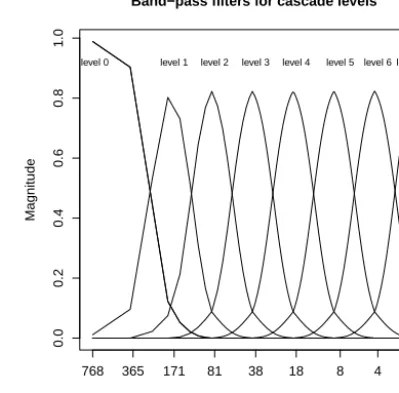
the number of cascade levels. A buffer of 64 pixels is added at each side of the original 256×256 grid in an attempt to reduce the edge effects arising from the FFT transformation, thus giving a larger domain of 384×384 pixels. The cas-cade is multiplicative when rewritten in terms of original rain ratesRinstead of the multiplicative decibel scale dBR. The cascade decomposition is achieved by applying a Gaussian band-pass filter to isolate a given set of spatial scales in the frequency domain (Seed, 2003; see Fig. 2). Xk will be

re-ferred to as cascade level and is obtained by applying an in-verse FFT to the filtered data in order to return the Fourier components back into the spatial domain. Thus, Xk

repre-sents the variability of the original radar field with spatial fre-quencies [km−1] in the rangeqk−1/L < ωk< qk+1/L, where

ωkis the central frequency of the Gaussian filter andq=2.12

is the branching number (inverse of the scale reduction fac-tor). Each level of the cascade is normalized to zero mean and unit variance for convenience and the normalization is kept constant in space and during the forecast period.

Figure 2 illustrates the Gaussian band-pass filters that are used to isolate the spatial scales composing the set of cas-cade levels. Given the size of the extended radar domain, an eight-level multiplicative cascade with the following spatial scales is obtained (see Fig. 2): 768–362, 362-171-81, 171-81-38, 81-38-18, 38-18-8, 18-8-4, 8-4-2 and 4-2 km. The non-integer scales resulting from the non-non-integer branching num-ber of 2.12 were rounded. The scales on which the Gaussian filters are centered are marked in italic. The first and last lev-els of the cascade will not be considered in the analyses be-cause of not having a regular Gaussian shape. In addition, the largest scale is not able to capture the appropriate scales since the radar composite only covers a certain fraction of the 512×512 km2domain. This would lead to the underestima-tion of the precipitaunderestima-tion lifetime at that scale (see Sect. 3.3). 3.2 Lagrangian temporal auto-correlation

The Lagrangian temporal auto-correlation is a measure for the rate of development of precipitation in storm coordinates and consequently of its predictability (Zawadzki, 1973). An efficient way to follow the rainfall evolution in storm coor-dinates is to estimate a velocity field using a sequence of radar rainfall fields. STEPS uses an optical flow algorithm (Bowler et al., 2004) for the estimation of the velocity field and a semi-Lagrangian backward-in-time scheme for its ad-vection, which keeps the velocity field fixed and retrieves the rainfall values upstream by following the lines of the velocity field (e.g., Germann and Zawadzki, 2002).

0.0

0.2

0.4

0.6

0.8

1.0

Band−pass filters for cascade levels

Spatial scale [km]

Magnitude

768 365 171 81 38 18 8 4 2

level 0 level 1 level 2 level 3 level 4 level 5 level 6 level 7

Figure 2. The set of eight Gaussian band-pass filters used to

iso-late the spatial frequencies composing the cascade levels. The total magnitude for a given spatial frequency is normalized to one.

The Lagrangian lag 1 temporal auto-correlations at each level of the cascade are estimated as follows (Bowler et al., 2006):

1. Estimate the velocity field with optical flow using rain-fall fields at timet−1 andt.

2. Decompose the radar rainfall field at time t−1 using FFT into a multiplicative cascade.

3. Decompose the radar rainfall field at timet using FFT into a multiplicative cascade.

4. Advect the cascade from timet−1 to timet. Note that each level of the cascade is advected with the same ve-locity field computed on the original rainfall fields. 5. The lag 1 Lagrangian temporal auto-correlation is

sim-ply obtained by computing the correlation coefficient between each cascade levelkadvected from timet−1 totand the corresponding cascade level at timet:

ρ1(k)=

1

L·L

L P

i=1

L P

j=1

Xkij−Xk·

X_kijadv−Xadvk

v u u

t_L1_·L

L P

i=1

L P

j=1

Xkij−Xk

v u u

t_L1_·L

L P

i=1

L P

j=1

Xadv_kij−Xadv_k

fork=1, . . ., K−1, (2)

as well by advecting a cascade at timet−2 to timet, but is not presented in this paper.

Equation (2) is the ordinary Pearson’s correlation coef-ficient, which involves the subtraction of the field mean. On the other hand, Zawadzki (1973) and Germann and Za-wadzki (2002) employed a correlation estimation without subtraction of the mean for estimating the decorrelation time of precipitation fields. The difference between the two ap-proaches is not very important over continental scales, where the forecast and observed fields have similar mean values, but it may become an issue over smaller domains, where the ob-served mean field precipitation can be significantly different than the forecast one (see, e.g., Foresti et al., 2012). In such a case, Eq. (2) would give lower but more realistic correlation coefficients compared with Germann and Zawadzki (2002).

The Lagrangian auto-correlation estimations are also af-fected by the presence of different scales of motion. A mul-tiscale optical flow estimation at each level of the cascade may be foreseen but could cause algorithm convergence is-sues when one is trying to correlate the small-scale features. Also, it is not yet clear how to avoid the appearance of arti-facts in the final reconstructed rainfall field when advecting the cascade levels with different velocity fields over several time steps.

Note that the correlation function of Eq. (2) is obtained by integrating over space, i.e., over the total number of pix-elsL·Lwithin a radar image. This allows the Lagrangian auto-correlation to be estimated in real time and to adapt to the predictability of the sequence of radar images. This ap-proach, however, assumes the predictability to be homoge-neous over the forecast domain. Section 3.4 will explain how to obtain estimates of the Lagrangian auto-correlation by per-forming the summations through time, which is a necessary step for analyzing its spatial distribution.

The hierarchy of Lagrangian temporal auto-correlations defines a hierarchy of auto-regressive processes of order 1 – AR(1). This is exploited by STEPS to stochastically simulate the rainfall growth and decay processes that occur in storm coordinates at different spatial scales to reproduce the dy-namic scaling of the field (Seed, 2003; Bowler et al., 2006). The procedure consists of blending the radar cascade with a cascade of spatially and temporally correlated stochastic noise. The spatially correlated noise field is generated us-ing a power law filter while temporal correlations are main-tained by a hierarchy of auto-regressive processes. The power law filter ensures that the noise cascade has the same power spectrum of the observed radar rainfall fields. This technique was already employed to generate continuous multifractals (Schertzer and Lovejoy, 1987) and also appeared in the now-casting system SBMcast (Berenguer et al., 2011), based on the “String of Beads” model of Pegram and Clothier (2001a). The stochastic simulations are stationary and no attempt is made to actually forecast temporal trends in growth and cay of precipitation. Indeed, trying to predict growth and

de-cay processes using as predictor the past evolution of radar precipitation does not seem to significantly improve the fore-cast accuracy, except for the regions characterized by sys-tematic orographic forcing (see a review in Foresti and Seed, 2014). In addition, Radhakrishna et al. (2012) showed that the predictability of growth and decay patterns is 10 times shorter than that of precipitation fields and is limited to spa-tial scales of the order of 250×250 km2, which would re-quire continental-scale radar images to be studied properly. The stochastic simulations are not presented in this paper but only explained for completeness since they are based on the Lagrangian auto-correlation coefficients.

3.3 Estimation of the precipitation lifetime

By knowing the lag 1 auto-correlation coefficient, the AR(1) auto-correlation function (ACF) can be recursively derived as follows:

ρ(t )=ρ₁t fort=1, . . ., T , (3)

where ρ1 is the lag 1 Lagrangian auto-correlation coeffi-cient computed with Eq. (2). Note that this simplification in-directly assumes that the diagnosed velocity field does not change during the forecast period. In fact, it extrapolates the whole ACF knowing only the lag 1 auto-correlation. This as-sumption is reasonable up to 2–3 h (Germann et al., 2005) and 3–4 h lead times (Bowler et al., 2006), since using the correct velocity does not reduce the forecast errors much. A complete study of the Lagrangian predictability of precip-itation including the non-stationarity of the velocity field, would involve the direct calculation of the correlation co-efficients at each forecast lead time by comparing the fore-casts to the observations (see Germann and Zawadzki, 2002). The basic principle of STEPS is to actually estimate the La-grangian ACF in real time and allow it to adapt to the pre-dictability of the situation. It would be computationally in-tensive to estimate the complete ACF using a few hours of radar fields before the analysis time. Eventually, the pre-dictability of the field would be representative of the previ-ous hours and not of the last two or three rainfall fields. The adaptability of the system is particularly important, for ex-ample, when the field is rapidly evolving from a convective to a stratiform situation or in the early stages of a new rainfall event.

Finally, the lifetime of precipitation (decorrelation time) can be evaluated by integrating the ACF over time (Zawadzki, 1973; Germann and Zawadzki, 2002):

LT =

∞ Z

0

ρ(t )dt. (4)

function, the integral of Eq. (4) can be analytically derived and is equal to− 1

ln(ρ0).

In order to generalize the methodology to different ACFs and for the comparison of observed and forecast field at all lead times, Eq. (4) was numerically integrated using the ex-tended Simpson’s rule (Press et al., 2007).

3.4 Online collection of rainfall statistics

Instead of analyzing the temporal distribution of the La-grangian auto-correlation by integrating the data over space, we want to analyze its spatial distribution by integrating over time. More precisely, the summations of Eq. (2) need to be done over the number of radar images in the archive, not the number of pixels within a radar image. A joint evaluation of the summations at each pixel in a radar field is intractable as it would require loading the whole archive of rainfall fields into the computer memory to compute the correlations in a single pass. An efficient way to overcome this issue is to ex-ploit rules for the online computation of the mean, the vari-ance and the covarivari-ance (Knuth, 1998). The online estima-tion of the mean is obtained as follows:

xt+1=xt+δ/N, (5)

wheret is the iteration,xt+1is the new mean,δ=xt+1−xt

is the residual contribution of the new samplext+1to the old meanxt andNis the number of samples.

The online estimation of the variance is obtained similarly as follows:

qt+1=qt+δ (xt+1−xt+1) , (6)

whereq is the squared sum of the differences ofx from its mean andδ=xt+1−xt. The variance is obtained offline by

dividingqby the number of samplesN.

The online computation of the AR(1) Lagrangian temporal auto-correlation is evaluated by keeping track of the sum of squared residuals:

st+1=st+

x_t+adv₁−xadv_t ·xt+1−xt+1

. (7)

The Lagrangian auto-correlation is obtained offline as:

ρx, xadv= s

N

q

Var(x)·Var xadv

. (8)

The online computation of statistics using these rules gradu-ally converges towards a stable value as the time progresses. In order to admit temporal fluctuations of the statistics and local smoothing, one can introduce a weight in the recursive equations similarly to the technique of recursive least squares computation.

The technical implementation of the online update of the field statistics is performed by keeping binary files contain-ing the arrays of interim statistics. For each new radar field,

the old file is read, updated and rewritten with the new statis-tics. The statistics are only updated when the rainfall frac-tion exceeds 5 % over the radar composite and when the four radars are jointly operating. With this criterion we ob-tained 9578 valid rainfall fields, which roughly correspond to 1600 h of precipitation over the period spanning from Febru-ary 2011 to October 2012.

3.5 Offline spectral slope estimation

A precipitation field that is scale-invariant (also referred to as

scaling) typically exhibits a power spectrum of the form:

P (f )∝f−β, (9)

wheref is the spatial frequency (km−1) andβis the scaling exponent (the slope of the power spectrum). The power law behavior of rainfall fields usually appears as a straight line on a graph of the logarithm of the power against the loga-rithm of the spatial frequency. The slope of the line measures the degree of scaling of the field and is equal to 0 for an unstructured white noise field. The scaling exponent of a 2-dimensional rainfall field is often greater than 2, which com-plicates its multifractal simulation (see, e.g., Schertzer and Lovejoy, 1987). One possibility to simulate stochastic rain-fall fields to obtainβ >2 is to apply a power law filter to a field of white noise as briefly mentioned in Sect. 3.2.

Radar rainfall fields often deviate from the theoretical framework of perfect scale-invariance and typically show a scaling break at frequencies of 15–20 km−1(see, e.g., Gires et al., 2011; Seed et al., 2013). On the other hand, precipi-tation fields computed by NWP models have a break around 40–50 km (e.g., Gires et al., 2011). The scaling break is ob-served as an increase in the spectral slope at the smaller con-vective scales. This seems to have a physical origin and could be attributed to different scaling regimes of the large-scale stratiform rainfall and the smaller convective scales. How-ever, recent analyses explain this phase transition with the presence of zeros in the field, which also affects the estima-tion of universal multifractal parameters (Gires et al., 2012). The presence of a scaling break requires using two spectral slopesβ1andβ2 for the study and parameterization of the power spectrum.β1accounts for wavelengths that are larger than 15–40 km andβ2for wavelengths that are lower than 15–40 km.

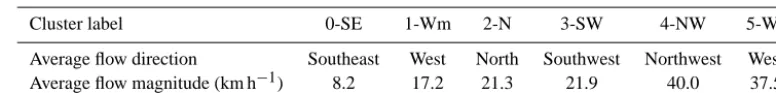
Table 1. Characteristics of the six flow cluster centers that are used to stratify the statistics. Wm and Ws refer to moderate and strong westerly

flows respectively. The detailed average velocity maps can be found in Foresti and Seed (2014).

Cluster label 0-SE 1-Wm 2-N 3-SW 4-NW 5-Ws

Average flow direction Southeast West North Southwest Northwest West

Average flow magnitude (km h−1) 8.2 17.2 21.3 21.9 40.0 37.5

deviations:

H= − 1

K−1

K−1

X

k=1

log₁₀ sd(Xkij) sd(X(k+1)ij)

log₁₀(q)

andβ=2H+E, (10)

where sd(Xkij) is the standard deviation of cascade levelkat

pixelij andE=2 is the dimension of the space.β1is esti-mated using levels 1 to 3 (scales of 171, 81 and 38 km,K=3 in Eq. 10) whileβ2using levels 3 to 6 (scales of 38, 18, 8 and 4 km;K=4 in Eq. 10). A scaling break of 40 km instead of

20 km was chosen to obtain smoother fields of the spectral exponentβ2, which is consequently slightly underestimated. Note that this approach is different than estimating power spectra on rainfall time series and analyzing the spatial distri-bution of the spectral exponents. The approach proposed in this paper should give insights into the spatial heterogeneity of the degree of spatial scaling of rainfall fields.

3.6 K-means stratification of optical flow fields

To analyze the dependence of rainfall statistics on flow regimes, the optical flow fields were stratified using the k-means clustering algorithm. The details on the preparation of the archive of optical flow fields and the clustering algorithm can be found in Foresti and Seed (2014).

Table 1 summarizes the statistics of the six cluster centers obtained after running the k-means algorithm on the archive of flow fields. The cluster centers mainly differ in terms of flow direction and magnitude, while the spatial variability of the velocity vectors within a field is only marginal (see Foresti and Seed, 2014). The number of clusters was empiri-cally chosen to represent a sufficient number of flow regimes and to have enough samples per cluster to compute signifi-cant verification statistics. The cluster 0 is characterized by weak southeasterly winds, the cluster 1 by moderate westerly winds, the cluster 2 by moderate northerlies, the cluster 3 by moderate southwesterly winds, the cluster 4 by strong north-westerly winds, and the cluster 5 by strong westerlies. It is understood that winds refer to the apparent motion of radar images derived with optical flow and not to real wind fields.

The online update of the statistics (Sect. 3.4) is per-formed by keeping a set of six binary files containing the interim fields of the rainfall mean, variance, Lagrangian auto-correlations and number of samples. The files are read,

up-dated and rewritten according to the cluster membership of a given field.

4 Results

Section 4.1 illustrates the scale-dependent geographical dis-tribution of the precipitation lifetime without stratification into flow regimes. On the other hand, Sect. 4.2 shows the flow dependence of the dynamic and spatial scaling relation-ships by averaging the results over space. Finally, Sect. 4.3 analyzes the spatial distribution of the precipitation lifetime under different flow regimes to understand the effect of oro-graphic forcing.

4.1 Geographical distribution of precipitation predictability and spatial scaling

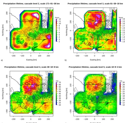
Figure 3 illustrates the spatial distribution of the precipitation lifetime for the cascade levels 2, 3, 4, and 5 without strati-fication into flow regimes. Refer to Fig. 1 for geographical details. The level 0 is not presented since the FFT filter does not have a Gaussian shape (see Fig. 2). On the other hand, the level 1 is too influenced by the edge effects that prop-agate from the borders of the radar composite towards the interior regions. The levels 6 and 7 are too noisy and exhibit lifetimes that are below the temporal resolution of the radar composite (10 min).

−200 −100 0 100 200 −200 −100 0 100 200

Precipitation lifetime, cascade level 2, scale 171−81−38 km

Easting [km] Nor thing [km] 2 3 4 5 6 7 8 9 10 11 12 200 200 200 200 400 400 400 400 400

600 600 600

600

800 800 800 800 1000 1000 1000 1000 1500 Melbourne Yarrawonga Gippsland hours a)

−200 −100 0 100 200

−200

−100

0

100

200

Precipitation lifetime, cascade level 3, scale 81−38−18 km

Easting [km] Nor thing [km] 1.00 1.25 1.50 1.75 2.00 2.25 2.50 2.75 3.00 3.25 3.50 200 200 200 200 400 400 400 400 400

600 600 600

600

800 800 800 800 1000 1000 1000 1000 1500 Melbourne Yarrawonga Gippsland hours b)

−200 −100 0 100 200

−200

−100

0

100

200

Precipitation lifetime, cascade level 4, scale 38−18−8 km

Easting [km] Nor thing [km] 20 25 30 35 40 45 50 55 60 65 70 200 200 200 200 400 400 400 400 400

600 600 600

600

800 800 800 800 1000 1000 1000 1000 1500 Melbourne Yarrawonga Gippsland min c)

−200 −100 0 100 200

−200

−100

0

100

200

Precipitation lifetime, cascade level 5, scale 18−8−4 km

Easting [km] Nor thing [km] 10 12 14 16 18 20 22 24 26 28 30 200 200 200 200 400 400 400 400 400

600 600 600

600

800 800 800 800 1000 1000 1000 1000 1500 Melbourne Yarrawonga Gippsland min d)

Figure 3. Spatial distribution of the precipitation lifetimes for the four middle cascade levels. (a) 171-81-38 km, (b) 81-38-18 km, (c) 38-18-8

and (d) 18-8-4 km. White tones are used for regions outside the radar domain or presenting values that exceed the range of the color scale.

less pronounced, this pattern was already observed by Foresti and Seed (2014) and is a consequence of the prevailing west-erly flows, which cause systematic rainfall decay on the lee-ward side of the Macedon ranges and orographic enhance-ment on their windward side. This effect is also the origin of the long lifetimes observed on the Dandenong ranges as they are located upwind relative to the prevailing westerlies. The lifetimes surrounding the Gippsland radar tend to be longer over the ocean, which is particularly visible in Fig. 3b and c. Finally, the shorter lifetimes on the inner parts of the Vic-torian Alps are probably due to the reduced accuracy of the radar measurements (see Sect. 2). In particular, the blockage of radar beams, the rainfall attenuation and overshooting re-duce the accuracy of the optical flow estimations, which con-sequently affects the lifetimes derived from the Lagrangian auto-correlation. In addition, it seems that there is a propor-tional effect between the precipitation lifetime and the

cli-matological precipitation amount: the lifetimes are generally lower in the places where the radar measures less precipita-tion (see e.g., Berenguer and Sempere-Torres, 2013).

−200 −100 0 100 200

−200

−100

0

100

200

Spectral slope, beta 1

Easting [km]

Nor

thing [km]

1.3 1.4 1.5 1.6 1.7 1.8 1.9 2.0 2.1 2.2 2.3 2.4

200

200

200

200 400

400 400 400

400

600 600 600

600

800 800 800

800

1000

1000

1000

1000

1500

Melbourne Yarrawonga

Gippsland

a)

−200 −100 0 100 200

−200

−100

0

100

200

Spectral slope, beta 2

Easting [km]

Nor

thing [km]

2.2 2.3 2.4 2.5 2.6 2.7 2.8 2.9 3.0

200

200

200

200 400

400 400 400

400

600 600 600

600

800 800 800

800

1000

1000

1000

1000

1500

Melbourne Yarrawonga

Gippsland

b)

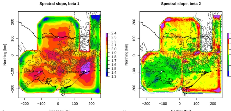
Figure 4. Spatial distribution of the spectral slopes (a)β1and (b)β2derived by assuming the scaling of the standard deviation of the cascade

levels.

the Alps located northeast of the Gippsland radar. This de-picts a region characterized by rainfall fields that are highly organized in space with convection embedded into stratiform rainfall, which is typical of orographic rainfall (see Fig. 6a). It would be interesting to perform a similar analysis using outputs from NWP models to eliminate the heterogeneities introduced by the inhomogeneous quality of radar measure-ments. As expected, the spectral slopes at the small scales (β2, Fig. 4b) are systematically higher than the ones at the large scales (β1, Fig. 4a), with values in the range 2.3–2.8. However, the spectral slopeβ2is lower in the surroundings of the Melbourne radar (S-band) compared with the other two (C-band). Both the C- and S-band radars have a 1◦ az-imuth and 250 m range resolution (see for instance, Ren-nie, 2012). Notwithstanding the same resolution, the rain-fall field exhibits more power in the last cascade level in the surroundings of the Melbourne radar, which can explain the lower spectral exponentβ2(Fig. 4b). The patterns observed in Fig. 4b are hard to explain in terms of different precip-itation regimes and seem to be more associated to the type of radar or data processing chain. Despite these differences, the spectral exponentsβ2tend to be lower upwind than up-stream of the mountain ranges, in particular over the Yarra and Dandenong ranges, the southern slopes of the Alps be-tween Avon and the Snowy River, and on the northern slopes of the Alps located southeast of the Yarrawonga radar. This depicts that strong convection is more likely to occur over flat regions than over complex orography, where it is less intense and often embedded into stratiform rainfall.

4.2 Flow dependence of the dynamic and spatial scaling relationships

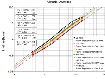
Table 2 and Fig. 5 illustrate the dynamic scaling relation-ship between the spatial scale and the precipitation lifetime

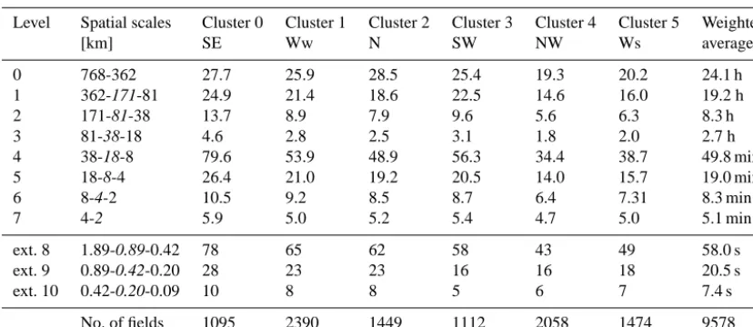
Table 2. Precipitation lifetimes for each spatial scale and flow regime averaged over the radar composite. Levels 0–3 are expressed in hours

and 4–7 in minutes. The power law extrapolation of lifetimes for smaller spatial scales is given in seconds. Ext.: estimation of the lifetimes at smaller spatial scales by extrapolating the power law. The extrapolation uses the original non-integer scales for increased precision. The scales on which the Gaussian filters are centered are marked in italic.

Level Spatial scales Cluster 0 Cluster 1 Cluster 2 Cluster 3 Cluster 4 Cluster 5 Weighted

[km] SE Ww N SW NW Ws average

0 768-362 27.7 25.9 28.5 25.4 19.3 20.2 24.1 h

1 362-171-81 24.9 21.4 18.6 22.5 14.6 16.0 19.2 h

2 171-81-38 13.7 8.9 7.9 9.6 5.6 6.3 8.3 h

3 81-38-18 4.6 2.8 2.5 3.1 1.8 2.0 2.7 h

4 38-18-8 79.6 53.9 48.9 56.3 34.4 38.7 49.8 min

5 18-8-4 26.4 21.0 19.2 20.5 14.0 15.7 19.0 min

6 8-4-2 10.5 9.2 8.5 8.7 6.4 7.31 8.3 min

7 4-2 5.9 5.0 5.2 5.4 4.7 5.0 5.1 min

ext. 8 1.89-0.89-0.42 78 65 62 58 43 49 58.0 s

ext. 9 0.89-0.42-0.20 28 23 23 16 16 18 20.5 s

ext. 10 0.42-0.20-0.09 10 8 8 5 6 7 7.4 s

No. of fields 1095 2390 1449 1112 2058 1474 9578

field over the continental United States. In Fig. 5 the 4–8 km scales roughly correspond to the 8-4-2 km and 18-8-4 scales, which exhibit lifetimes of 0.1–0.4 h.

To obtain an order of magnitude for the predictability at smaller spatial scales, power law relationships were fit-ted using the method of least squares per each flow cluster. The extrapolation of the fitted power laws towards smaller spatial scales could give an idea of the minimum tempo-ral resolution that is required to reliably measure the La-grangian auto-correlation of precipitation, which is very important for stochastic precipitation nowcasting at urban scales (e.g., Goormans and Willems, 2013; Ruzanski and Chandrasekar, 2012). The bottom of Table 2 shows the re-sults of such extrapolations for scales of 1.89-0.89-0.42, 0.89-0.42-0.20 and 0.42-0.20-0.09 km. Because of working on a logarithmic scale such estimations are quite uncertain and to a certain degree pessimistic, in particular because the dynamic scaling relationship does not perfectly follow a power law. The imperfect dynamic scaling could also be due to using the lifetime instead of the temporal rainfall changes as a measure for the rainfall evolution (see Venugopal et al., 1999). It must also be considered that the optical flow is representative of the scales measured by the C- and S-band radars and cannot capture the motion at smaller scales. From this simple extrapolation, the kilometric scale (1.89-0.89-0.42 km) only displays a predictability of 40–80 s. It would be interesting to study whether the temporal resolution of X-band radars is sufficient to reliably measure the Lagrangian auto-correlation of the very small scale precipitation features. Using such high resolution data will also pose the computa-tional challenge of generating the nowcasts before the pre-dictability limits have been exceeded to avoid the forecasts becoming obsolete. Ruzanski and Chandrasekar (2012)

re-ported a predictability of 20 min using data from a network of X-band radars and the CASA nowcasting system. The scale dependence was analyzed by upscaling the forecasts and the values are not directly comparable to the ones obtained by scale separation within STEPS. At these temporal scales, the quality of the nowcasts is still strongly affected by the accu-racy of the input radar observations. Therefore, it becomes necessary to complement nowcasting systems with heuristic models of the radar measurement uncertainty, for example to account for stochastic sampling errors (Jordan et al., 2003).

Table 3 illustrates the spectral slopesβ1andβ2of the spa-tial power spectrum stratified by flow regime.β1 typically oscillates around the dimension of the field with the small-est values occurring under the flows SE–SW (1.88–1.91) and the largest under the flows Wm, N, and NW (2.01–2.03). The values are slightly smaller than the ones found in the literature (e.g., Seed et al., 2013), which is explained again by the presence of edge effects that locally reduce the spec-tral exponents (see Fig. 4a). This may have consequences on the power law filtering performed by STEPS to generate the noise cascade needed to update the hierarchy of auto-regressive processes. In fact, the filtering uses the spatial power spectrum of rainfall as target distribution, which does not account for the spatial heterogeneities within the forecast domain.

Table 3. Average spatial spectral exponents stratified by flow regime. The standard deviation over space is given in brackets.

Cluster label 0-SE 1-Wm 2-N 3-SW 4-NW 5-Ws

β1 1.88 (0.29) 2.02 (0.24) 2.03 (0.25) 1.91 (0.22) 2.03 (0.24) 1.96 (0.23)

β2 2.46 (0.20) 2.55 (0.15) 2.61 (0.18) 2.46 (0.19) 2.79 (0.16) 2.68 (0.18)

1 10 100 1000

0.01 0.1 1 10 100

f(x) = 0.016 x^1.334 R² = 0.996 f(x) = 0.014 x^1.342 R² = 0.996 f(x) = 0.019 x^1.386 R² = 0.997 f(x) = 0.020 x^1.336 R² = 0.997 f(x) = 0.021 x^1.352 R² = 0.997 f(x) = 0.026 x^1.383 R² = 0.993

Precipitation lifetime as a function of scale and flow direction, Victoria, Australia

SE flows

Power Regression for SE flows Wm flows

Power Regression for Wm flows N flows

Power Regression for N flows SW flows

Power Regression for SW flows NW flows

Power Regression for NW flows Ws flows

Power Regression for Ws flows

Spatial scale [km]

L

ife

tim

e

[h

o

ur

s]

Wm

N

SW

NW

Ws SE

Figure 5. Dynamic scaling relationship between the spatial scale and precipitation lifetime stratified by flow regime. The equations of the

power law fits are shown in the upper left corner.

4.3 Effect of orography on the predictability of precipitation

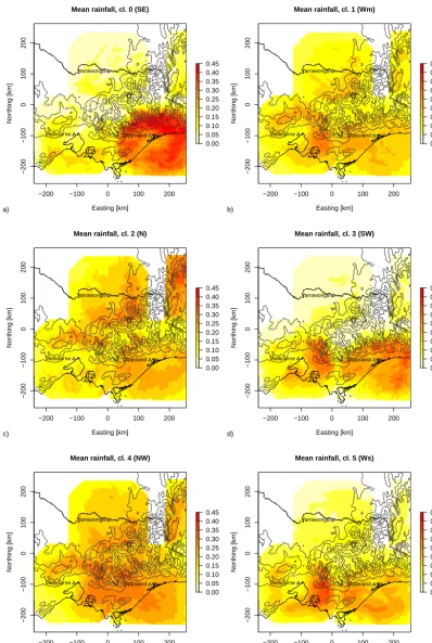
According to the results of Berenguer and Sempere-Torres (2013), the regions of long predictability seem to be correlated with the regions with the highest rainfall accumu-lations. In fact, the regions that are often affected by orga-nized large-scale precipitation systems are more likely to ex-hibit higher predictability than the ones with infrequent iso-lated convection. It is therefore important to analyze the cli-matology of precipitation to study the spatial distribution of its predictability.

Figure 6 shows the conditional mean 10 min rainfall ac-cumulations stratified by flow regime. It clearly illustrates the flow dependence of the spatial distribution of precip-itation, which is mostly located on the windward side of mountain ranges. Most of the precipitation occurring under southeasterly flows is located along the upwind side of the Victorian Alps in a region going from Avon to the Snowy River (Fig. 6a). The spatial distribution of rainfall under

moderate westerly flows presents maxima on the Dandenong and Macedon ranges, but also on the northern side of the Alps around Mount Buffalo (Fig. 6b). The enhancement on the Northwest flank of the Alps is much more pronounced with northerly and northwesterly flows, which approach the mountain range more perpendicularly (Fig. 6c and e, respec-tively). Southwesterly flows lead to high accumulations on the Yarra and Dandenong ranges as well as the southern side of the Alps around the Gippsland radar (Fig. 6d). It is inter-esting to note that northwesterly flows also give high accu-mulations on the leeside of the Alps (Fig. 6e), which could be caused by the lower air stability of these conditions (refer to Foresti and Seed, 2014, for a more detailed interpretation). Finally, strong westerly flows lead again to high accumula-tions on the Dandenong and Macedon ranges, but also on the West of the Gippsland radar (Fig. 6f). A clear rainfall shadow effect on the leeside of the Macedon ranges is noticed for the clusters Wm, NW, and Ws.

−200 −100 0 100 200 −200 −100 0 100 200

Mean rainfall, cl. 0 (SE)

Easting [km] Nor thing [km] 0.00 0.05 0.10 0.15 0.20 0.25 0.30 0.35 0.40 0.45 200 200 200 200 400 400 400 400 400

600 600 600

600

800 800 800 800 1000 1000 1000 1000 1500 Melbourne Yarrawonga Gippsland a)

−200 −100 0 100 200

−200

−100

0

100

200

Mean rainfall, cl. 1 (Wm)

Easting [km] Nor thing [km] 0.00 0.05 0.10 0.15 0.20 0.25 0.30 0.35 0.40 0.45 200 200 200 200 400 400 400 400 400

600 600 600

600

800 800 800 800 1000 1000 1000 1000 1500 Melbourne Yarrawonga Gippsland b)

−200 −100 0 100 200

−200

−100

0

100

200

Mean rainfall, cl. 2 (N)

Easting [km] Nor thing [km] 0.00 0.05 0.10 0.15 0.20 0.25 0.30 0.35 0.40 0.45 200 200 200 200 400 400 400 400 400

600 600 600

600

800 800 800 800 1000 1000 1000 1000 1500 Melbourne Yarrawonga Gippsland c)

−200 −100 0 100 200

−200

−100

0

100

200

Mean rainfall, cl. 3 (SW)

Easting [km] Nor thing [km] 0.00 0.05 0.10 0.15 0.20 0.25 0.30 0.35 0.40 0.45 200 200 200 200 400 400 400 400 400

600 600 600

600

800 800 800 800 1000 1000 1000 1000 1500 Melbourne Yarrawonga Gippsland d)

−200 −100 0 100 200

−200

−100

0

100

200

Mean rainfall, cl. 4 (NW)

Easting [km] Nor thing [km] 0.00 0.05 0.10 0.15 0.20 0.25 0.30 0.35 0.40 0.45 200 200 200 200 400 400 400 400

400

600 600 600

600

800 800 800 800 1000 1000 1000 1000 1500 Melbourne Yarrawonga Gippsland e)

−200 −100 0 100 200

−200

−100

0

100

200

Mean rainfall, cl. 5 (Ws)

Easting [km] Nor thing [km] 0.00 0.05 0.10 0.15 0.20 0.25 0.30 0.35 0.40 0.45 200 200 200 200 400 400 400 400

400

600 600 600

600

800 800 800 800 1000 1000 1000 1000 1500 Melbourne Yarrawonga Gippsland f)

by flow cluster. Despite some variability arising from peri-odic features of the Fourier transform, it is possible to notice that lifetimes are higher on the upwind side and lower on the downwind side of terrain features. An illustrative example can be observed under southwesterly conditions (Fig. 7d). The lifetime of precipitation upstream of the Dandenong ranges is about 20–40 min; it increases to 50–70 min on the upwind side and falls again to 20–30 min when moving into the Alps. Similar patterns can be observed under the flow regime Ws (Fig. 7f). On the other hand, under NW flows short lifetimes are located on the leeward side of the Mace-don ranges (Fig. 7e). Note that with reversed flow conditions (SE, Fig. 7a), this region exhibits lifetimes of 80–100 min and the shortest ones are located on top of the Macedon ranges with values oscillating between 40 and 80 min. The region located South and Southeast of the Yarrawonga radar is also interesting to analyze in particular for the clusters N and NW. In fact, the location of the longest lifetimes up-stream of the Alps is different depending on flow direction (Fig. 7c and e). The plains surrounding the Yarrawonga radar also show very long lifetimes under flow conditions SE, Wm, and SW. However, this effect could be an artefact of the low rainfall accumulations over these regions (see Fig. 6a, b, and d).

These findings corroborate the results of Harris et al. (1996), who demonstrated that the precipitation intermit-tency is higher upstream compared with the top of the moun-tain ridge, with intermediate values on the upwind flank. From Fig. 7 it seems that the decreased intermittency of rain-fall upwind of orographic features has a positive impact on its predictability by Lagrangian persistence. It is worth men-tioning that leeside precipitation enhancement is also pos-sible due to leeside flow convergence, flow perturbations by mountain gravity waves, or the presence of cold air pools that force the unstable air to rise. Such processes are not very fre-quent and would require stratifying the statistics using more complex criteria based on moist air stability indices among others.

The relationship between the precipitation lifetime and orography is less pronounced than that of nowcast biases presented in Foresti and Seed (2014). This is mostly due to the increased difficulty in computing higher order statis-tics, which require many more samples than a simple lin-ear or multiplicative bias. Also, the cascade decomposition framework still needs some improvements to reduce the edge effects and to better interpret the intricate statistical depen-dencies between consecutive cascade levels (see Seed et al., 2013).

5 Conclusions

The geographical distribution of the scale-dependent pre-dictability of precipitation by Lagrangian extrapolation of radar images was analyzed under different flow regimes

in connection with the presence of orographic features. Data from the Victorian radar composite, Australia, a 500×500 km2 domain covering the period from Febru-ary 2011 to October 2012, were used for the analyses. The scale dependence of the predictability of precipitation was considered by decomposing the radar rainfall field into a multiplicative cascade using an FFT (Bowler et al., 2006). The lifetime of precipitation features was found to be a power law function of the scale of the features and to depend on flow direction, which confirms the presence of dynamic scaling (Venugopal et al., 1999; Mandapaka et al., 2009). The pre-cipitation lifetime was found to be up to a factor of 2 higher on the upwind compared with the downwind slopes of oro-graphic features and to be strongly flow-dependent. The de-gree of spatial scaling of the rainfall field was also shown to be spatially inhomogeneous. These spatial heterogeneities due to orographic forcing can be exploited to locally adapt the space–time stochastic simulation of precipitation, which is needed for very short-term forecasting (e.g., Seed et al., 2013), generating radar ensembles (Germann et al., 2009), design storm studies (e.g., Paschalis et al., 2013), and precip-itation downscaling (e.g., Pathirana and Herath, 2002).

The study raised several methodological questions, in par-ticular because the quality of radar data is much more homo-geneous over time than over space. This has to be accounted for when interpreting the maps of the predictability of precip-itation. Some patterns could be simply due to the geograph-ical biases that affect the radar measurements, for example due to beam blockage, signal attenuation, or increasing sam-pling volume with range. Nevertheless, in the regions close to the radar, it was possible to detect a clear signal in the dis-tribution of the precipitation lifetime, which was attributed to orographic forcing.

The predictability estimates presented in this paper are af-fected by other sources of uncertainty. The first is related to the assumption of the temporal stationarity of the diag-nosed velocity field, which leads to over-optimistic estimates of the precipitation lifetimes, especially at the large scales. The second arises from the uncertainty in the estimation of the velocity field with optical flow. In fact, precipitation fields often show differential motion at different spatial scales. An illustrative example occurs when stationary orographic rain-fall contains fast moving cellular convection (e.g., Foresti et al., 2013). Better estimates of the Lagrangian predictability would require the optical flow to be estimated on each spatial scale separately.

−200 −100 0 100 200 −200 −100 0 100 200

Precipitation lifetime, cl. 0 (SE), level 4, scale 38−18−8 km

Easting [km] Nor thing [km] 40 50 60 70 80 90 100 110 120 130 140 200 200 200 200 400 400 400 400 400

600 600 600

600

800 800 800 800 1000 1000 1000 1000 1500 Melbourne Yarrawonga Gippsland min a)

−200 −100 0 100 200

−200

−100

0

100

200

Precipitation lifetime, cl. 1 (Wm), level 4, scale 38−18−8 km

Easting [km] Nor thing [km] 30 35 40 45 50 55 60 65 70 75 80 200 200 200 200 400 400 400 400 400

600 600 600

600

800 800 800 800 1000 1000 1000 1000 1500 Melbourne Yarrawonga Gippsland min b)

−200 −100 0 100 200

−200

−100

0

100

200

Precipitation lifetime, cl. 2 (N), level 4, scale 38−18−8 km

Easting [km] Nor thing [km] 30 35 40 45 50 55 60 65 70 75 80 200 200 200 200 400 400 400 400 400

600 600 600

600

800 800 800 800 1000 1000 1000 1000 1500 Melbourne Yarrawonga Gippsland min c)

−200 −100 0 100 200

−200

−100

0

100

200

Precipitation lifetime, cl. 3 (SW), level 4, scale 38−18−8 km

Easting [km] Nor thing [km] 30 35 40 45 50 55 60 65 70 75 80 85 90 200 200 200 200 400 400 400 400 400

600 600 600

600

800 800 800 800 1000 1000 1000 1000 1500 Melbourne Yarrawonga Gippsland min d)

−200 −100 0 100 200

−200

−100

0

100

200

Precipitation lifetime, cl. 4 (NW), level 4, scale 38−18−8 km

Easting [km] Nor thing [km] 20 25 30 35 40 45 50 55 60 65 70 200 200 200 200 400 400 400 400 400

600 600 600

600

800 800 800 800 1000 1000 1000 1000 1500 Melbourne Yarrawonga Gippsland min e)

−200 −100 0 100 200

−200

−100

0

100

200

Precipitation lifetime, cl. 5 (Ws), level 4, scale 38−18−8 km

Easting [km] Nor thing [km] 20 25 30 35 40 45 50 55 60 65 70 200 200 200 200 400 400 400 400 400

600 600 600

600

800 800 800 800 1000 1000 1000 1000 1500 Melbourne Yarrawonga Gippsland min f)

which would enable the nowcasting system to learn about the spatial distribution of predictability as more and more radar data are collected and analyzed.

Acknowledgements. This research was funded by the Swiss

National Science Foundation (SNSF) project “Data mining for pre-cipitation nowcasting” (PBLAP2-127713/1). We also would like to acknowledge the Belgian Science Policy Office (BELSPO) project PLURISK: “Forecasting and management of rainfall-induced risks in the urban environment” (SD/RI/01A), which allowed this study to be finalized. Urs Germann is specially thanked for the discussion on the predictability of precipitation. We acknowledge Mark Curtis and Kevin Cheong for the technical support received, and Maarten Reyniers and Laurent Delobbe for reviewing the manuscript.

Edited by: H. Leijnse

References

Badas, M. G., Deidda, R., and Piga, E.: Modulation of ho-mogeneous space-time rainfall cascades to account for oro-graphic influences, Nat. Hazards Earth Syst. Sci., 6, 427–437, doi:10.5194/nhess-6-427-2006, 2006.

Berenguer, M., and Sempere-Torres, D.: Radar-based rainfall now-casting at European scale: long-term evaluation and performance assessment, Proc. of the 36th AMS Conf. on Radar Meteorology, Breckenridge, Colorado, USA, 2013.

Berenguer, M., Sempere-Torres, D., and Pegram, G. G. S.: SBMcast – An ensemble nowcasting technique to assess the uncertainty in rainfall forecasts by Lagrangian extrapolation, J. Hydrol., 404, 226–240, 2011.

Bousquet, O., Lin, C. A., and Zawadzki, I.: Analysis of scale depen-dence of quantitative precipitation forecast verification: a case-study over the Mackenzie river basin, Q. J. Roy. Meteorol. Soc., 132, 2107–2125, 2006.

Bowler, N. E. H., Pierce, C. E., and Seed, A. W.: Development of a precipitation nowcasting algorithm based upon optical flow tech-niques, J. Hydrol., 288, 74–91, 2004.

Bowler, N. E. H., Pierce, C. E., and Seed, A. W.: STEPS: A prob-abilistic precipitation forecasting scheme which merges an ex-trapolation nowcast with downscaled NWP, Q. J. Roy. Meteorol. Soc., 132, 2127–2155, 2006.

Casati, B., Ross, G., and Stephenson, D. B.: A new intensity-scale approach for the verification of spatial precipitation forecasts, Meteorol. Appl., 11, 141–154, 2004.

Chumchean, S., Sharma, A., and Seed, A.: An integrated approach to error correction for real-time radar-rainfall estimation, J. At-mos. Ocean. Tech., 23, 67–79, 2006a.

Chumchean, S., Seed, A., and Sharma, A.: Correcting of real-time radar rainfall bias using a Kalman filtering approach, J. Hydrol., 317, 123–137, 2006b.

Chumchean, S., Seed, A., and Sharma, A.: An operational approach for classifying storms in real-time radar rainfall estimation, J. Hydrol., 363, 1–17, 2008.

Foresti, L. and Seed, A.: On the spatial distribution of rainfall nowcasting errors due to orographic forcing. Meteorol. Appl., doi:10.1002/met.1440, in press, 2014.

Foresti, L., Kanevski, M., and Pozdnoukhov, A.: Kernel-based mapping of orographic rainfall enhancement in the Swiss Alps as detected by weather radar, IEEE T. Geosci. Remote, 50, 2954–2967, 2012.

Foresti, L., Panziera, L., Mandapaka, P. V., Germann, U., and Seed, A.: Retrieval of analogue radar images for ensemble nowcasting of orographic rainfall, Meteoforol. Appl., doi:10.1002/met.1416, in press, 2013.

Germann, U. and Zawadzki, I.: Scale-dependence of the pre-dictability of precipitation from continental radar images, Part I: Methodology, Mon. Weather Rev., 130, 2859–2873, 2002. Germann, U., Zawadzki, I., and Turner, B.: Scale-dependence of

the predictability of precipitation from continental radar images, Part IV: Limits to Prediction, J. Atmos. Sci., 63, 2092–2108, 2006.

Germann, U., Berenguer, M., Sempere-Torres, D., and Zappa, M.: REAL – Ensemble radar precipitation estimation for hydrol-ogy in a mountainous region, Q. J. Roy. Meteorol. Soc., 135, 445–456, 2009.

Gires, A., Tchiguirinskaia, I., Schertzer, D., and Lovejoy, S.: Mul-tifractal and spatio-temporal analysis of the rainfall output of the Meso-NH model and radar data, Hydrolog. Sci. J., 55, 380–396, 2011.

Gires, A., Tchiguirinskaia, I., Schertzer, D., and Lovejoy, S.: In-fluence of the zero-rainfall on the assessment of the multifractal parameters, Adv. Water Resour., 45, 13–25, 2012.

Goormans, T. and Willems, P.: Using local weather radar data for sewer system modeling: case study in Flanders, Belgium, J. Hy-drol. Eng., 18, 269–278, 2013.

Grecu, M. and Krajewski, W. F.: A large-sample investigation of statistical procedures for radar-based short-term quantitative pre-cipitation forecasting, J. Hydrol., 239, 69–84, 2000.

Harris, D., Menabde, M., Seed, A., and Austin, G.: Multifractal characterization of rain fields with a strong orographic influence, J. Geophys. Res., 101, 26405–26414, 1996.

Huuskonen, A., Saltikoff, E., and Holleman, I.: The operational radar network in Europe, B. Am. Meteorol. Soc., 95, 897–907, doi:10.1175/BAMS-D-12-00216.1, 2014.

Jordan, P., Seed, A. W., and Weinnman, P. E.: A stochastic model of radar measurement errors in rainfall accumulations at catchment scale, J. Hydrometeorol., 4, 841–855, 2003.

Knuth, D. E.: The Art of Computer Programming, in: volume 2: Seminumerical Algorithms, 3rd Edn, Addison-Wesley, Boston, 1998.

Lorenz, E. N.: Predictability of flow which possesses many scales of motion, Tellus, 21, 289–307, 1969.

Mandapaka, P. V., Lewandowski, P., Eichinger, W. E., and Kra-jewski, W. F.: Multiscaling analysis of high resolution space-time lidar-rainfall, Nonlin. Processes Geophys., 16, 579–586, doi:10.5194/npg-16-579-2009, 2009.

Marsan, D., Schertzer, D., and Lovejoy, S.: Causal space-time mul-tifractal processes: Predictability and forecasting of rain fields, J. Geophys. Res., 101, 26333–26346, 1996.

Panziera, L. and Germann, U.: The relation between airflow and orographic precipitation on the southern side of the Alps as revealed by weather radar, Q. J. Roy. Meteorol. Soc., 136, 222–238, 2010.

Paschalis, A., Molnar, P., Fatichi, S., and Burlando, P.: A stochastic model for high-resolution space-time precip-itation simulation, Water Resour. Res., 49, 8400–8417, doi:10.1002/2013WR014437, 2013.

Pathirana, A. and Herath, S.: Multifractal modelling and simulation of rain fields exhibiting spatial heterogeneity, Hydrol. Earth Syst. Sci., 6, 695–708, doi:10.5194/hess-6-695-2002, 2002.

Pegram, G. G. S. and Clothier, A. N.: High resolution space-time modelling of rainfall: the “String of Beads” model, J. Hydrol., 241, 26–41, 2001a.

Pegram, G. G. S. and Clothier, A. N.: Downscaling rainfields in space and time, using the String of Beads model in time series mode, Hydrol. Earth Syst. Sci., 5, 175–186, doi:10.5194/hess-5-175-2001, 2001b.

Press, W. H., Teukolsky, S. A., Vetterling, W. T., and Flannery, B. P.: Numerical Recipes: The Art of Scientific Computing, 3rd Edn., Cambridge University Press, 2007.

Radhakrishna, B., Zawadzki, I., and Fabry, F.: Predictability of pre-cipitation from continental radar images, Part V: growth and decay, J. Atmos. Sci., 69, 3336–3349, doi:10.1175/JAS-D-12-029.1, 2012.

Rennie, S. J.: Doppler weather radar in Australia, CAWCR techni-cal report, no. 055, Centre for Australian Weather and Climate Research, Melbourne, Australia, 2012.

Ruzanski, E. and Chandrasekar, V.: An investigation of the short-term predictability of precipitation using high-resolution com-posite radar observations, J. Appl. Meteorol., 51, 912–925, 2012. Schertzer, D. and Lovejoy, S.: Physical modelling and analysis of rain and clouds by anisotropic scaling multiplicative processes, J. Geophys. Res., 92, 9696–9714, 1987.

Seed, A.: A dynamic and spatial scaling approach to advection fore-casting, J. Appl. Meteorol., 42, 381–388, 2003.

Seed, A. and Pegram, G. G. S.: Using Kriging to infill gaps in radar data due to ground clutter in real-time. Proceedings of the 5th Int. Symp. on Hydrological Applications of Weather Radar, Kyoto, Japan, 73–78, 2001.

Seed, A., Duthie, E., and Chumchean, S.: Rainfields: the Australian Bureau of Meteorology system for quantitative precipitation es-timation, Proc. of the 33rd Conf. on Radar Meteorology, Cairns, Australia, 2007.

Seed, A. W., Pierce, C. E., and Norman, K.: Formulation and eval-uation of a scale decomposition-based stochastic precipitation nowcast scheme, Water Resour. Res., 49, 6624–6641, 2013. Sinclair, S. and Pegram, G. G. S.: Empirical Mode

Decompo-sition in 2-D space and time: a tool for space-time rainfall analysis and nowcasting, Hydrol. Earth Syst. Sci., 9, 127–137, doi:10.5194/hess-9-127-2005, 2005.

Surcel, M., Zawadzki, I., and Yau, M. K.: On the filtering prop-erties of ensemble averaging for storm-scale precipitation fore-casts, Mon. Weather Rev., 142, 1093–1105, 2014.

Turner, B. J., Zawadzki, I., and Germann, U.: Predictability of pre-cipitation from continental radar images, Part III: operational nowcasting implementation (MAPLE), J. Appl. Meteorol., 43, 231–248, 2004.

Venugopal, V., Foufoula-Georgiou, E., and Sapozhnikov, V.: Ev-idence of dynamic scaling in space-time rainfall, J. Geophys. Res., 104, 31599–31610, 1999.

Zawadzki, I. I.: Statistical properties of precipitation patterns, J. Appl. Meteorol., 12, 459–472, 1973.