Deriving inherent optical properties and associated inversion uncertainties in the Dutch Lakes

www.hydrol-earth-syst-sci.net/13/1113/2009/ © Author(s) 2009. This work is distributed under the Creative Commons Attribution 3.0 License.

Earth System

Sciences

Deriving inherent optical properties and associated

inversion-uncertainties in the Dutch Lakes

M. S. Salama1, A. Dekker2, Z. Su1, C. M. Mannaerts1, and W. Verhoef1,3

1_{International Institute for Geo-Information Science and Earth Observation, Enschede, The Netherlands} 2_{Commonwealth Scientific and Industrial Research Organisation, Australia}

3_{The National Aerospace Laboratory NLR, Emmeloord, The Netherlands}

Received: 13 February 2009 – Published in Hydrol. Earth Syst. Sci. Discuss.: 9 March 2009 Revised: 24 June 2009 – Accepted: 1 July 2009 – Published: 13 July 2009

Abstract. Remote sensing of water quality in inland waters requires reliable retrieval algorithms, accurate atmospheric correction and consistent method for uncertainty estimation. In this paper, the GSM semi-analytical inversion model is modified for inland waters to derive inherent optical prop-erties (IOPs) and their spectral dependencies from air and space borne data. The modified model was validated using two data sets from the Veluwe and the Vecht Dutch lakes. For the Veluwe lakes, the model was able to derive a linear relationship between measured concentrations and estimated IOPs withR2values above 0.7 for chlorophyll-a(Chl-a) and up to 0.9 for suspended particulate matters (SPM). In the Vecht lakes, the modified model derived accurate values of IOPs. TheR2values were 0.89 for Chl-aand up to 0.95 for SPM. The RMSE values were 0.93 mg m−3_{and 0.56 g m}−3 for Chl-a and SPM respectively. Finally, the IOPs of the Veluwe lakes are derived from multi-spectral, ocean color and hyperspectral airborne data. Inversion-uncertainties of the derived IOPs were also estimated using a standard non-linear regression technique. The study shows that inversion-uncertainties of remote sensing derived IOPs are proportional to water turbidity.

1 Introduction

Lakes are important natural water resources yet they are se-riously threatened by eutrophication, salinisation and heavy metal contamination. Increased sediment loads paly an im-portant role in water quality of lakes since they relate total primary production to heavy metal and micro pollutants (Vos et al., 1998). Traditional measurements of water quality are costly, time-consuming and are limited in their spatial and

Correspondence to: M. S. Salama ([email protected])

of the derived IOPs following previous researchers (Salama, 2003; Wang et al., 2005; Maritorena and Siegel, 2005).

2 Method

The total remote sensing reflectance received at the sensor level can be written as the sum of several components (Gor-don, 1997):

Rst(λ)=Rsr(λ)+Rsa(λ)+Tv(λ){Rssfc(λ)+Rsw(λ)}(1) whereTv(λ) is the viewing diffuse transmittance from the water surface to the sensor. The subscript of the reflectance represents the contribution from air molecules r, aerosol a, surface sfc, and water w. The calculation of Rayleigh scat-tering of air molecules is well described in terms of geom-etry and pressure (Gordon et al., 1988a). Water surface re-flectance can be estimated using statistical relationships and wind speed (Cox and Munk, 1954a,b). Gaseous transmit-tance can be calculated from ancillary data on ozone and wa-ter vapor content using transmittance models (Goody, 1964; Malkmus, 1967). Viewing diffuse transmittance is approx-imated following Gordon et al. (1983). Aerosol scattering can be evaluated from measured aerosol optical thickness and assumed aerosol type. This information about the atmo-spheric path reflectance facilitates the retrieval of the signal leaving the water body i.e.Rsw. Water remote sensing re-flectanceRsw(λ)can be related to the inherent optical prop-erties (IOPs) of the water column as (GSM model: Mari-torena et al., 2002):

Rsw(λ)=

t n2

w 2

X

i=1

gi

bb(λ) bb(λ)+a(λ)

i

(2)

whereg1,g2are subsurface expansion coefficients due to in-ternal refraction, reflection and sun zenith;t andnware the sea air transmission and water index of refraction, respec-tively. Their values are taken from literature (Gordon et al., 1988b; Maritorena et al., 2002; Lee, 2006). The parameters

bb(λ) anda(λ) are the bulk backscattering and absorption

coefficients of the water column. Case II water is consid-ered with three independently varying constituents, namely: chlorophyll-a(Chl-a), detritus and dissolved organic matter (dg) and suspended particulate matter (SPM). The absorption and backscattering coefficients are modeled as being the sum of absorption and backscattering from all water constituents:

a(λ)=aw(λ)+aph(λ)+adg(λ) (3)

bb(λ)=0.5bw(λ)+αbspm(λ) (4)

The absorption and scattering coefficients of water molecules, aw and bw, were assumed constants. Their values were obtained from (Pop and Fry, 1997; Mobley, 1994), respectively.

The total absorption of phytoplankton pigmentsaphis ap-proximated as (Lee et al., 1999):

aph(λ)=a0(λ)aph(0.44)+a1(λ)aph(0.44)lnaph(0.44) (5) wherea0(λ)anda1(λ) are empirical coefficients. The ab-sorption effects of detritus and dissolved organic matter are combined due to the similar spectral signature (Maritorena et al., 2002) and approximated using the model (Bricaud et al., 1981):

adg(λ)=adg(440)exp [−s(λ−440)] (6) where s is an unknown spectral exponent. The scattering coefficient of SPM bspm is parameterized as (Kopelevich, 1983):

bspm(λ)=bspm(550)

₅₅₀

λ

y

(7) where y is the unknown spectral shape parameter. The backscattering fractionαis estimated from the “San Diego harbor” scattering phase function (Petzold, 1977).

The inversion of the GSM model is adapted to derive five parameters in visible bands covering the wavelengths from 400 nm to 850 nm. These parameters are called the set of IOPs and denoted as a vector iop:

iop= 

    

aph(440)

adg(440)

bspm(550)

s y



    

(8)

The Levenberg-Marquardt Algorithm (LMA) is employed using a constrained nonlinear optimization (Press et al., 2002). The constraints are set such that they guarantee posi-tive values of retrieved IOPs. Both parameters, concentration and absorption/(back)scattering coefficients, are denoted us-ing the same abbreviation of the constituent itself i.e., dg, Chl-a, SPM.

3 Materials

3.1 Field measurements and study areas

400 500 600 700 800 900 0

0.002 0.004 0.006 0.008 0.01 0.012 0.014 0.016 0.018

wavelength nm

w

a

te

r

le

a

v

in

g

r

e

fl

e

c

ta

n

c

e

%

P1 P2 P3 P4 P5 P6 P7 P8

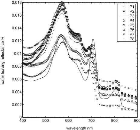
Fig. 1.Measured water leaving reflectance in the Veluwe lakes during the EAGLE 2006 campaign.

17

Fig. 1. Measured water leaving reflectance in the Veluwe lakes

dur-ing the EAGLE 2006 campaign.

Table 1. Locations of the sampling sites and measured

concentra-tions in the Veluwe lakes during the EAGLE 2006 campaign.

site Lat Long SPM g m−3 Chl-amg m−3

P1 52.37481 5.63524 5.84 10.4

P2 52.38326 5.63874 4.47 6.8

P3 52.37735 5.65598 1.86 2.3

P4 52.37566 5.66849 3.04 5.7

P5 52.39295 5.65845 2.78 9.4

P6 52.38732 5.64361 3.96 6.2

P7 52.37570 5.62356 3.44 6.7

P8 52.36788 5.63584 0.93 4.2

The second set consists of measured under-water irradiance reflectance, inherent optical properties and concentrations of water constituents at 20 sites in the Vecht lakes, centered at 52◦1009.000N, 05◦10015.000E. Data on the optical and physi-cal properties of the Vecht lakes were obtained from Dekker (1993) and Dekker et al. (1997).

3.2 Remote sensing data set

The EAGLE 2006 campaign was associated with hyperspec-tral airborne measurements from the Airborne Hyperspec-tral Spectrometer (AHS) (Fern´andez-Renau et al., 2005). MEdium Resolution Imaging Spectrometer (MERIS) and Advanced Space borne Thermal Emission and Reflection Ra-diometer (ASTER) observations were also available during the EAGLE 2006 campaign. Table 2 summarizes the used data sets in this work. For more details on data availabilities and specifications, the reader is encouraged to consult the

0.4 0.6 0.8 1

−2 −1 0 1 2 3

Measured C

ph mg.m

−3

Derived log(a

p

(440) [m

−1

])

R2_=0.74

(a)

0 0.2 0.4 0.6 0.8

0.2 0.4 0.6 0.8 1

Measured C SPM g.m

−3

Derived log(b

spm

(550) [m

−1])

R2_=0.91

(b)

Fig. 2. Comparison between the derived IOPs and measured concentrations in the Veluwe lakes of(a):

chlorophyll-aand(b): SPM. The bold line is a linear regression through the data. The dashed lines denote

the 95% confidence interval of the regression results. TheR2_{values are for the data points.}

18

Fig. 2. Comparison between the derived IOPs and measured

con-centrations in the Veluwe lakes of (a): chlorophyll-aand (b): SPM. The bold line is a linear regression through the data. The dashed lines denote the 95% confidence interval of the regression results. TheR2values are for the data points.

EAGLE 2006 data acquisition reports (Timmermans et al., 2007; Su et al., 2009) and the works of Dekker (1993) and Dekker et al. (1997).

4 Results

4.1 Model validation

The modified inversion model is validated with in-situ mea-surements in the Veluwe and the Vecht lakes. Figure 2 shows the derived IOPs versus measured concentrations in the Veluwemeer and Wolderwijd, i.e. the Veluwe lakes. There is a strong linear relationship between derived IOPs and measured concentrations. TheR2values of model-I re-gression (Laws, 1997) is about 0.74 and 0.9 for

chlorophyll-a and SPM respectively. Following the Lambert-Beer law one can easily derive the specific inherent optical properties (SIOPs) of chlorophyll-a and SPM, i.e. the amount of ab-sorption/scattring per unit concentration. For demonstration, the regression line and the 95% confidence interval between the IOPs and corresponding concentrations are also shown in Fig. 2.

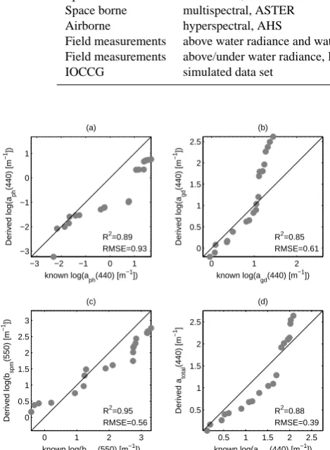
Figure 3 shows derived versus measured values of IOPs in the Vecht lakes. Four IOPs are shown: three absorption coef-ficientsaph(440),adg(440),atotal(440)and one scattering co-efficientbspm(550). Model II regression (Laws, 1997) is used to evaluate the match between derived and measured values in Table 3 for log-transformed data. The derived IOPs are within acceptable accuracy, i.e. theR2is higher than 0.85 for the four derived IOPs. The derived scattering coefficient at 550 nm has the highest accuracy with RMSE value less than 0.56 g m−3andR2∼0.95. The uncertainties in the retrieved absorption coefficients are large, particularly the value of

Table 2. Summary of the data sets used in this study.

Acquisition Type Description Date

Space borne ocean color, MERIS FR level L1b 08-06-2006

Space borne multispectral, ASTER level L1b 08-06-2006

Airborne hyperspectral, AHS Level L1b 13-06-2006

Field measurements above water radiance and water samples Veluwe lakes 04-07-2006 Field measurements above/under water radiance, IOPs and water samples Vecht lakes 1993–1997

IOCCG simulated data set spectra and IOPs 2006

−3 −2 −1 0 1

−3 −2 −1 0 1

known log(a

ph(440) [m

−1 ])

Derived log(a

ph

(440) [m

−1

])

R2=0.89

RMSE=0.93 (a)

0 1 2

0 0.5 1 1.5 2 2.5

known log(a

gd(440) [m

−1 ])

Derived log(a

gd

(440) [m

−1

])

R2=0.85

RMSE=0.61 (b)

0 1 2 3

0 0.5 1 1.5 2 2.5 3

known log(b

spm(550) [m

−1_])

Derived log(b

spm

(550) [m

−1

])

R2_=0.95

RMSE=0.56 (c)

0.5 1 1.5 2 2.5

0.5 1 1.5 2 2.5

known log(a total(440) [m

−1_])

Derived a

total

(440) [m

−1

]

R2_=0.88

RMSE=0.39 (d)

Fig. 3.Comparison between the derived and measured values in the Vecht lakes of(a): chlorophyll-aabsorption coefficient at 440 nm,(b): dg absorption coefficient at 440 nm,(c): SPM scattering coefficient at 550 nm and

(d): total absorption coefficient at 440 nm. The bold line denote the 1:1 line.

19

Fig. 3. Comparison between the derived and measured values in the

Vecht lakes of (a): chlorophyll-aabsorption coefficient at 440 nm,

(b): dg absorption coefficient at 440 nm, (c): SPM scattering

coeffi-cient at 550 nm and (d): total absorption coefficoeffi-cient at 440 nm. The bold line denote the 1:1 line.

4.2 Intercomparison of remotely sensed products

Available images during the EAGLE 2006 campaign are geo-referenced and converted to at-sensor-reflectance. At-mospheric path correction is then preformed using the ra-diative transfer method of Vermote et al. (1997). Gaseous transmittances of ozone, oxygen, carbon dioxide, methane and nitrous oxide are assumed constant over the study re-gion. Measured values of aerosol optical thickness during the the EAGLE 2006 campaign are used to run the com-putation, assuming an urban aerosol. The adjacency ef-fects from the surrounding lands was accounted for in the computation. The IOPs are derived using the constrained LMA. This method is applied on MERIS and AHS spec-tra, while another method is used for ASTER image. The

Table 3. RMSE and type-II regression parameters between

mea-sured and derived IOPs in the Vecht Lakes.nis the number of data points.

Parameter n Intercept Slope R2 RMSE

aph(440) 20 −0.73 0.83 0.89 0.93 adg(440) 20 −0.58 1.98 0.85 0.61 a(440) 20 −0.54 1.40 0.88 0.39

bspm(550) 20 0.37 0.67 0.95 0.56

spectral characteristics of ASTER constrain the application of such nonlinear fit method. There are several methods that were successfully applied to ASTER and other sensors with few visible bands (Kishino et al., 2005; Salama et al., 2004). For ASTER’s two visible bands, the matrix inversion method (Hoge and Lyon, 1996) was applied assuming known value ofadg(440)=0.25 m−1. In consequence only two vari-ables were retrieved from ASTER image, namely SPM scat-tering and Chl-a absorption coefficients. An intercompari-son between retrieved values of SPM scattering and Chl-a

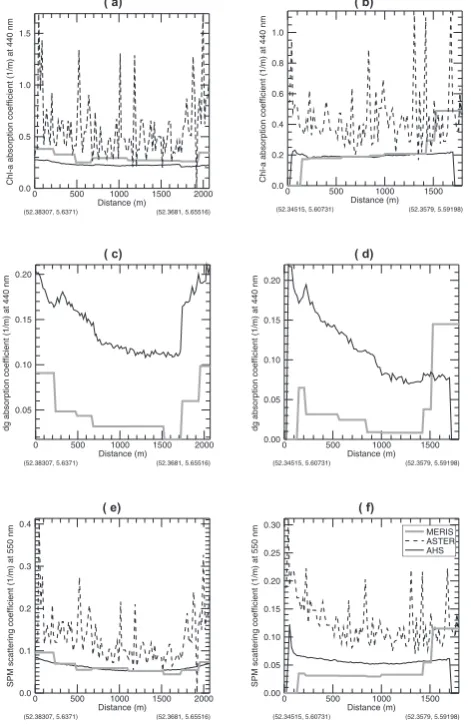
and dg absorptions are shown in Fig. 4 for two cross sections over the Veluwemeer (start 52.38307, 5.63710, end 52.3681, 5.65516) and the Wolderwijd (start 52.34515, 5.60731, end 52.3579, 5.59198). There is a very good match between the products of AHS and MERIS while retrieved values from ASTER are patchy and don’t correspond to derived IOPs from other sensors.

4.3 Inversion-uncertainties of AHS derived IOPs

( c)

( b)

( e) ( f)

( d) ( a)

Fig. 5.Intercomparison of IOPs derived from MERIS (gray thick-line), ASTER (dashed line) and AHS (black

thin-line) for a cross-section at the Veluwemeer (Fig.a, c, e) and a cross-section at the Wolderwijd (Fig.b, d,

f). The derived IOPs are: Chl-a(a and b), dg (c and d) and SPM (e and f).

21

Fig. 4. Intercomparison of IOPs derived from MERIS (gray

thick-line), ASTER (dashed line) and AHS (black thin-line) for a cross-section at the Veluwemeer (Fig. a, c, e) and a cross-cross-section at the Wolderwijd (Fig. b, d, f). The derived IOPs are: Chl-a(a and b), dg (c and d) and SPM (e and f).

inversion-uncertainty maps of IOPs have similar spatial vari-ations and their values increase proportionally to water tur-bidity as shown in Fig. 6.

5 Discussion

5.1 Validation

For the Veluwe lakes, the model was able to derive the linear relationship between measured concentrations and estimated IOPs. TheR2values of model-I regression were above 0.7 for chlorophyll-a and up to 0.9 for SPM. The SIOPs val-ues of the Veluwe lakes are not documented yet. There-fore, using reported values of SIOPs for other Dutch lakes, e.g. (Hakvoort et al., 2002), will lead to significant errors in the derived concentrations.

Fig. 6.The standard deviation (STD) maps for each of the retrieved IOPs from AHS data set of(a): Chl-a,(c):

dg and(e): SPM. Right panels (Fig.b, d, f) illustrate the scatter plot between standard deviations values on the

Y-axis and the corresponding IOPs values on the X-axis.

22

Fig. 5. The standard deviation (STD) maps for each of the retrieved

IOPs from AHS data set of (a): Chl-a , (c): dg and (e): SPM. Right panels (Fig. b, d, f) illustrate the scatter plot between standard deviations values on the Y-axis and the corresponding IOPs values on the X-axis.

Fig. 7.The standard deviation (STD) of derived:(a)Chl-aand(b)dg absorption coefficients as function of the estimated values of SPM scattering.

23

Fig. 6. The standard deviation (STD) of derived: (a) Chl-a and

(b) dg absorption coefficients as function of the estimated values of

SPM scattering.

for aph(440), adg(440)and bspm(550) respectively. How-ever, the modified model could not derive accurate IOPs val-ues when the scattering and absorption coefficients are above 20 m−1and 10 m−1respectively. We think that model param-eterizations in Eq. (5), Eq. (6) and Eq. (7) are not adequate for inland waters with extreme values of absorption and scat-tering. Each of these parameterizations poses one limitation on the model: (i) Eq. (5) ignores the different phytoplank-ton species that may co-exist in inland water; (ii) Eq. (5) also ignores the great variability of Chl-aabsorption as mea-sured in nature (Bricaud et al., 1995, 1998; Carder et al., 1999); (iii) Eq. (6) combines the absorption effect of detri-tus and CDOM in one spectral shape and magnitude; (iv) the overlapped absorption spectra of CDOM, detritus and Chl-a

at 440 nm will also encumber their retrievals. For instance, Fig. 3a and b show that the trend of derived Chl-aabsorption, w.r.t. actual values, is inversely correlated to that of derived absorption of CDOM and detritus, i.e. underestimated val-ues ofaph(440)are associated with overestimated values of

adg(440)and vice versa. The effects of over/under estima-tions will compensate each other when the total absorption coefficient is evaluated, as shown in Fig. 3d.

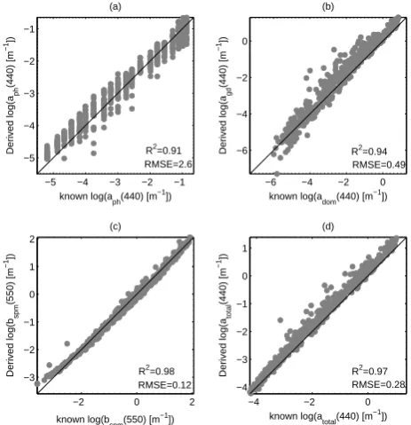
The consistency of the adapted inversion, with respect to the original GSM model, is analyzed using the same data set (Lee, 2006, IOCCG data set). Figure 7 shows derived versus known values of IOPs using the IOCCG data set. The sta-tistical parameters of model II regression (Laws, 1997) were also used to evaluate the match between derived and known values as shown in Table 4. The modified GSM succeeded in deriving the IOPs withR2 higher than 0.9 and 100% of valid retrievals from the IOCCG data set, for comparison one may consult (Lee, 2006, p. 83–84). Moreover, the valida-tion results of IOCCG data set are consistent with the val-idation results of in-situ measured parameters in the Vecht lakes: (i) derivedaph(440)has the highest RMSE; (ii) de-rived aph(440) andadg(440)are opposite to each other in their trends; (iii) the opposite trend ofaph(440)andadg(440) is compensated in theatot(440); (iv) the accuracy of SPM scattering is the highest among other derived IOPs.

−5 −4 −3 −2 −1

−5 −4 −3 −2 −1

known log(a

ph(440) [m

−1 ])

Derived log(a

ph

(440) [m

−1

])

R2_=0.91

RMSE=2.6 (a)

−6 −4 −2 0

−6 −4 −2 0

known log(a

dom(440) [m

−1 ])

Derived log(a

gd

(440) [m

−1

])

R2=0.94

RMSE=0.49 (b)

−2 0 2

−3 −2 −1 0 1 2

known log(b

spm(550) [m

−1 ])

Derived log(b

spm

(550) [m

−1

])

R2_=0.98

RMSE=0.12 (c)

−4 −2 0

−4 −3 −2 −1 0 1

known log(a total(440) [m

−1_])

Derived log(a

total

(440) [m

−1

])

R2_=0.97

RMSE=0.28 (d)

Fig. 4.Comparison between the derived and simulated IOCCG values of(a): chlorophyll-aabsorption

coef-ficient at 440 nm,(b): dg absorption coefficient at 440 nm,(c): SPM scattering coefficient at 550 nm and(d):

total absorption coefficient at 440 nm. The bold line denote the 1:1 line.

20

Fig. 7. Comparison between the derived and simulated IOCCG

val-ues of (a): chlorophyll-aabsorption coefficient at 440 nm, (b): dg absorption coefficient at 440 nm, (c): SPM scattering coefficient at 550 nm and (d): total absorption coefficient at 440 nm. The bold line denote the 1:1 line.

Table 4. RMSE and type-II regression parameters between known

and derived values form the IOCCG data set. nis the number of data points.

Parameter n Intercept Slope R2 RMSE

aph(440) 500 0.0039 0.92 0.91 1.15 a_dg(440) 500 0.0097 1.35 0.94 0.21

a(440) 500 −0.0041 1.27 0.97 0.12

bspm(550) 500 −0.0515 1.02 0.98 0.05

However the RMSE values between derived and measured data in the Vecht lakes are larger by three folds, for the ab-sorption, to an order of magnitude for the scattering. This increase in RMSE values is related to the optical-complexity of inland waters and emphasizes our previous findings that new parameterizations should be adapted for, case 2, inland waters.

5.2 Remotely sensed products

atmospheric correction methods. The derived values of SPM scattering and Chl-aabsorption from ASTER are patchy and did not reflect the spatial variability as observed from MERIS and AHS. This can be attributed to the retrieval method ap-plied on ASTER. The inversion of ASTER was based on matrix inversion of Eq. (2) in two bands with a constant value of dg absorption coefficient at 440 nm (=0.25 m−1). On the other hand, the retrieval method of MERIS and AHS was based on nonlinear optimization for five variables in all visible bands i.e. 15 for MERIS and 16 for AHS. There is a very good match in the retrieved values of SPM scat-tering at the Veluwemeer (Fig. 4e) and Chl-a absorptions at the Wolderwijd (Fig. 4b). However, slight overestima-tion of Chl-a absorption and underestimation of SPM scat-tering coefficients with-respect-to (w.r.t.) AHS can be ob-served in Fig. 4a and Fig. 4f respectively. The values of dg absorption coefficient are generally overestimated w.r.t. AHS retrieved values, with the same spatial variation, how-ever. The differences between MERIS and AHS results may be attributed to imperfect atmospheric correction and inap-propriate spectral coverage of AHS for Chl-a retrieval. On the one hand, the longer atmospheric path of MERIS w.r.t. AHS signals increases the contributions of aerosol scattering and illumination-viewing variations to the top of atmosphere (TOA) reflectance. It is also noted that AHS spectral range does not cover chlorophyll-a absorption feature centered at 440 nm. This absorption feature is of quite importance for reliable estimation of Chl-a and dg absorption coefficients. The combined effects of the longer atmospheric path and the absence of 440 nm absorption feature will increases the un-certainties on the retrieved values of dg and Chl-a. A ma-jor limitation in this work is that air and space borne images were not concurrent with field measurements such that in-dependent validation of remotely sensed products was not possible.

5.3 Inversion-uncertainties

The method of Bates and Watts (1988) was used to estimate the uncertainties of derived IOPs. However, this approach is adequate as long as model inversion has a well conditioned Jacobian matrix of the minimum cost function. It reflects how well the model can fit the observation but not how well the derived parameters fit the measured values. The esti-mated uncertainties (Fig. 5), therefore do not reflect the ac-tual uncertainties which are presented in Table 4 as RMSE values. This total uncertainty of derived values can roughly be assigned to three main causes: residuals, numerical and physical sources. Residuals are errors originated from sen-sor noise and imperfect atmospheric correction or any other correction. The numerical part is related to the used nu-meric technique in the inversion. The physical uncertainty is caused by two distinctive sources: bio-optical model ap-proximations and the intrinsic relation between apparent and inherent optical properties of the water column which causes

reflectance ambiguity. The later is an inherent problem to remote sensing of water quality (Sydor et al., 2004). In this sense, mainly model approximation and inversion accuracy were quantified in Fig. 5. Figure 5 shows that there are weak relationships between derived values of absorption co-efficients and associated uncertainties. This is not the case for the scattering where a clear relationship can be observed (Fig. 5c). The error increases exponentially with the magni-tude of derived values. Actually, the uncertainty of all IOPs increase proportionally to water turbidity (Fig. 6). There-fore, larger errors are expected in turbid waters. Two water types can be distinguished from the right panels of Fig. 5 and Fig. 6. The pixels within the gray region have STD values less than the value of the corresponding IOPs. These pixels correspond to relatively smaller range of derived IOPs. The remaining pixels, which form the majority, have their STD values higher than the retrieved values of IOPs, i.e. uncer-tainty is more than 100%. This grouping is caused by the large inversion errors in case 2 waters with large values of scattering and absorption. This was already predicted dur-ing model validation in the Vecht lakes, Fig. 3). This kind of comparison between derived values and their uncertainties has been found useful for resolving the sub-pixel variability of earth observation hydrological products (Van der Velde et al., 2008).

6 Conclusions

In this paper the GSM model was modified to retrieve five parameters: three IOPs and two spectral exponents. The method is applied on MERIS and AHS and validated using measured and IOCCG data sets. From the presented work in this paper we conclude the followings:

– The proposed modification improved the performance of the GSM model for simulated data and derived reli-able results for measured data.

– The red and NIR bands, with sufficient signal-to-noise ratio, are necessary for remote sensing of inland water. They improve the accuracy of derived IOPs.

– Improved parametrization of IOPs is needed for inland waters. The improvement should account for: (i) differ-ent phytoplankton species; (ii) the absorption of SPM as linked to the concentration.

Acknowledgements. The authors would like to thank the European Space Agency (ESA) for supporting this research and supplying MERIS data, the Instituto Nacional de T´ecnica Aeroespacial (INTA) for providing high quality hyperspectral dataset and techni-cal assistance, the National Aeronautics and Space Administration (NASA) for providing ASTER data, the EAGLE 2006 team for collecting and archiving in-situ measurements. The financial support of ESA, arrangement No. 20239/06/I-LG, is gratefully acknowledged. Emmanuel Boss, anonymous reviewer and Jun Wen are gratefully acknowledged for revising the manuscript and improving on its quality.

Edited by: J. Wen

References

Bates, D. and Watts, D.: Nonlinear regression analysis and its ap-plications, John Wiley and Sons, NY, 365 pp., 1988.

Bricaud, A., Morel, A., and Prieur, L.: Absorption by dissolved organic-matter of the sea (yellow substance) in the UV and visi-ble domains, Limnol. Oceanogr., 26, 43–53, 1981.

Bricaud, A., Babin, M., Morel, A., and Claustre, H.: Variability in the chlorophyll-specific absorption coefficients of naturnal phy-toplankton: Analysis and parameterization, J. Geophys. Res., 100, 13321–13332, 1995.

Bricaud, A., Morel, A., Babin, M., Allali, K., and Claustre, H.: Variations of light absorption by suspended particles with chloro-phyll a concentration in oceanic (case 1) waters: Analysis and implications for bio-optical models, J. Geophys. Res., 103(C13), 31033–31044, 1998.

Carder, K., Chen, F., Lee, Z., Hawes, S., and Kamykowski, D.: Semianalytical Moderate-Resolution Imaging Spectrometer al-gorithms for chlorophyll-a and absorption with bio-optical do-mains based on nitrate-depletion temperature, J. Geophys. Res., 104, 5403–5421, 1999.

Cox, C. and Munk, W.: Measurements of the roughness of the sea surface from photographs of the sun glitter, J. Opt. Soc. Am., 44, 838–850, 1954a.

Cox, C. and Munk, W.: Statistics of the sea surface derived from sun glitter, J. Mar. Res., 13, 198–227, 1954b.

Dekker, A.: Detection of optical water quality parameters for eu-trophic waters by high resolution remote sensing, Ph.D. thesis, Vrije Universiteit, Amsterdam, 1993.

Dekker, A., Malthus, T., Wijnen, M., and Seyhan, E.: Remote sens-ing as a tool for assesssens-ing water quality in Loosdrecht Lakes, Hydrobiologia, 233, 137–159, 1992.

Dekker, A., Hoogenboom, H., Goddijn, L., Malthus, T.: The re-lationship between inherent optical properties and reflectance spectra in turbid inland waters, Remote Sens. Reviews, 15, 59– 74, 1997.

Doerffer, R. and Fischer, J.: Concentration of chlorophyll, sus-pended matter, and gelbstoff in case II waters derived from satel-lite coastal zone color scanner with inverse methods, J. Geophys. Res., 99, 7457–7466, 1994.

Doerffer, R. and Schiller, H.: The MERIS cas 2 water algorithm, Int. J. Remote Sens., 28, 3/4, 517–535, 2007.

Fern´andez-Renau, A., G´omez, J. A., and De Miguel, E.: The INTA-AHS system, in: SPIE proceeding of Sensors, Systems and Next-Generation Satellites IX, Vol. 5978, 471–478, 2005.

GEOSS: GEO Inland and nearshore coastal water quality remote sensing, in: GEOSS group on earth observation, edited by: Bauer, M., Dekker, A., DiGiacomo, P., Greb, S., Gitelson, A., Herlevi, A., and Kutser, T., GEO, 2007.

Gitelson, A., Garbuzov, G., Szilagyi, F., Mittenzwey, K. H., Karnieli, A., and Kaiser, A.: Quantitative remote sensing meth-ods for real-time monitoring of inland waters quality, Int. J. Re-mote Sens., 14, 1269–1295, 1993.

Gons, H., Rijkeboer, M., and Ruddick, K.: A chlorophyll-retrieval algorithm for satellite imagery (Medium Resolution Imaging Spectrometer) of inland and coastal waters, J. Plankton Res., 24, 947–951, 2002.

Goody, R.: Atmospheric radiation 1, theoretical basis, Oxford Uni-versity Press, 544 pp., 1964.

Gordon, H.: Atmospheric correction of ocean color imagery in the Earth Observing System era, J. Geophys. Res., 102, 17081– 17106, 1997.

Gordon, H., Clark, D., Brown, J., Brown, O., Evans, R., and Broenkow, W.: Phytoplankton pigment concentrations in the middle Atlantic bight: comparison of ship determinations and CZCS estimates, Appl. Optics, 22, 20–36, 1983.

Gordon, H., Brown, J., and Evans, R.: Exact Rayleigh scattering calculation for the use with the Nimbus-7 Coastal Zone Color Scanner, Appl. Optics, 27, 862–871, 1988a.

Gordon, H., Brown, O., Evans, R., Brown, J., Smith, R., Baker, K., and Clark, D.: A semianalytical radiance model of ocean color, J. Geophys. Res., 93(D9), 10909–10924, 1988b.

Hakvoort, H.: Absorption of light by surface water, Ph.d., Technis-che Universiteit, Delft, 1994.

Hakvoort, H., de Haan, J., Jordans, R., Vos, R., Peters, S., and Ri-jkeboer, M.: Towards airborne remote sensing of water quality in The Netherlands – validation and error analysis, ISPRS J. Pho-togramm., 57, 171–183, 2002.

Hoge, F. E. and Lyon, P. E.: Satellite retrieval of inherent optical properties by linear matrix inversion of ocean radiance models: An analysis of model and radiance measurement errors, J. Geo-phys. Res., 101, 16631–16648, 1996.

Hoogenboom, H., Dekker, A., and De Haan, J.: Retrieval of chloro-phyll a and suspended matter in inland waters from Casi data by matrix inversion, Can. J. Remote Sens., 24, 144–152, 1998. Kallio, K., Kutser, T., Hannonen, T., Koponen, S., Pulliainen, J.,

Vepsalainen, J., and Pyhalahti, T.: Retrieval of water quality from airborne imaging spectrometry of various lake types in different seasons, Sci. Total Environ., 208, 59–77, 2001.

Kishino, M., Tanaka, A., and Ishizaka, J.: Retrieval of Chloro-phyll a, suspended solids, and colored dissolved organic matter in Tokyo Bay using ASTER data, Remote Sens. Environ., 99, 66–74, 2005.

Kopelevich, O.: Small-parameter model of optical properties of sea waters, Vol. 1, Physical Ocean Optics, Nauka, 1983.

Laws, E.: Mathematical Methods for Oceanographers: An intro-duction, John Wiley and Sons, New York, 343 pp., 1997. Lee, Z. and Carder, K.: Hyperspctral remote sensing, in: Remote

Sensing of Coastal Aquatic Environments, edited by: Miller, R., del Castillo, C., and McKee, B., Springer, Dordrecht, The Netherlands, 181–204, 2005.

Lee, Z., Carder, K., Mobley, C., Steward, R., and Patch, J.: Hyper-spectral remote sensing for shallow waters: 2. Deriving bottom depths and water properties by optimization, Appl. Optics, 38, 3831–3843, 1999.

Malkmus, W.: Random Lorentz band model with exponential-tailed S−1 line intensity distribution function, J. Opt. Soc. Am., 57, 323–329, 1967.

Maritorena, S. and Siegel, D.: Consistent merging of satellite ocean color data sets using a bio-optical model, Remote Sens. Environ., 94, 429–440, 2005.

Maritorena, S., Siegel, D., and Peterson, A.: Optimization of a semianalytical ocean color model for global-scale applications, Appl. Optics, 41, 2705–2714, 2002.

Mobley, C.: Light and water radiative transfer in natural waters, Academic Press, 592 pp., 1994.

Petzold, T.: Volume scattering functions for selected ocean waters, in: Light in the Sea, edited by: Tyler, J., Dowden, Hutchinson and Ross, Stroudsburg, Pa. USA, Vol. 12, pp. 150–174, 1977. Pop, R. and Fry, E.: Absorption spectrum (380–700 nm) of pure

wa-ter: II, Integrating cavity measurements, Appl. Optics, 36, 8710– 8723, 1997.

Press, W., Teukolsky, S., Vetterling, W., and Flannery, B.: Numer-ical recipes in C++, The art of scientific computing, Cambridge University Press, 1002 pp., 2002.

Salama, M. S.: Optical remote sensing for the estimation of ma-rine bio-geophysical quantities, Ph.D. Thesis, Katholieke Uni-versiteit, Leuven, 2003.

Salama, M. S., Monbaliu , J., Coppin, P.: Atmospheric correction of Advanced Very High Resolution Radiometer imagery, Int. J. Remote Sens., 25, 7/8, 1349–1355, 2004.

Shen, F., Salama, M. S., Zhou, Y., Li, J., Su, Z., and Kuang, D.: Remote-sensing reflectance characteristics of highly turbid estu-arine waters – a comparative experiment of the Yangtze River and the Yellow River, Int. J. Remote Sens., in press, 2009.

Schroeder, T., Behnert, I., Schaale, R., Fischer, J., and Doerffer, R.: Atmospheric correction algorithm for MERIS above case-2 waters, Int. J. Remote Sens., 28, 7, 1469–1486, 2007.

Su, Z., Timmermans, W. J., van der Tol, C., Dost, R., Bianchi, R., G´omez, J. A., House, A., Hajnsek, I., Menenti, M., Magliulo, V., Esposito, M., Haarbrink, R., Bosveld, F., Rothe, R., Baltink, H. K., Vekerdy, Z., Sobrino, J. A., Timmermans, J., van Laake, P., Salama, S., van der Kwast, H., Claassen, E., Stolk, A., Jia, L., Moors, E., Hartogensis, O., and Gillespie, A.: EAGLE 2006 – Multi-purpose, multi-angle and multi-sensor in-situ and airborne campaigns over grassland and forest, Hydrol. Earth Syst. Sci., 13, 833–845, 2009,

http://www.hydrol-earth-syst-sci.net/13/833/2009/.

Sydor, M., Gould, R., Arnone, R., Haltrin, V., and Goode, W.: Uniqueness in remote sensing of the inherent optical properties of ocean water, Appl. Optics, 43, 2156–2162, 2004.

Timmermans, W., Dost, R., and Su, Z.: EAGLE 2006 – EAGLE Netherlands multi-purpose, multi-angle and multi-sensor in-situ, airborne and spaceborne campaigns over grassland and forest, Tech. rep., Department of Water Resources International Institute for Geo-Information Science and Earth Observation, ITC, 2007. Van der Velde, R., Su, Z., and Ma, Y.: Impact of soil moisture dynamics on ASAR so signatures and its spatial variability ob-served over the Tibetan Plateau, Sensors, 8, 5479–5491, 2008. Van der Woerd, H. and Pasterkamp, R.: HYDROPT: A fast and

flex-ible method to retrieve chlorophyll-afrom multispectral satellite observations of optically complex coastal waters, Remote Sens. Environ., 112, 1795–1807, 2008.

Vermote, E., Tanre, D., Deuze, J., Herman, M., and Morcrette, J.: Second simulation of the satellite signal in the solar spectrum, 6S: An overview, IEEE T. Geosci. Remote, 35, 675–686, 1997. Vos, R., Villars, M., Roozekrans, J., Peters, S., and Raaphorst,

W. V.: Integrated monitoring of total suspended sediment in the Dutch coastal zone, Tech. rep., part II, 1998.