Hydrol. Earth Syst. Sci., 13, 453–465, 2009 www.hydrol-earth-syst-sci.net/13/453/2009/ © Author(s) 2009. This work is distributed under the Creative Commons Attribution 3.0 License.
Hydrology and
Earth System
Sciences
An alternative deterministic method for the spatial interpolation of
water retention parameters
H. Saito1, K. Seki2, and J. ˇSim ˚unek3
1Department of Ecoregion Science, Tokyo University of Agriculture and Technology, Fuchu, Tokyo 183-8509, Japan 2Faculty of Business Administration, Toyo University, Tokyo 112-8606, Japan
3Department of Environmental Sciences, University of California, Riverside, CA 92521, USA
Received: 1 August 2008 – Published in Hydrol. Earth Syst. Sci. Discuss.: 3 September 2008 Revised: 31 March 2009 – Accepted: 31 March 2009 – Published: 7 April 2009
Abstract. There are two approaches available for mapping water retention parameters over the study area using a spatial interpolation method. (1) Retention models can be first fit-ted to retention curves available at sampling locations prior to interpolating model parameters over the study area (the FI approach). (2) Retention data points can first be interpolated over the study area before retention model parameters are fitted (the IF approach). The current study compares the per-formance of these two approaches in representing the spatial distribution of water retention curves. Standard geostatisti-cal interpolation methods, i.e., ordinary kriging and indicator kriging, were used. The data used in this study were obtained from the Las Cruces trench site database, which contains water retention data for 448 soil samples. Three standard water retention models, i.e., Brooks and Corey (BC), van Genuchten (VG), and Kosugi (KSG), were considered. For each model, standard validation procedures, i.e., leave-one-out cross-validation and split-sample methods were used to estimate the uncertainty of the parameters at each sampling location, allowing for the computation of prediction errors (mean absolute error and mean error). The results show that the IF approach significantly lowered mean absolute errors for the VG model, while also reducing them moderately for the KSG and BC models. In addition, the IF approach re-sulted in less bias than the FI approach, except when the BC model was used in the split-sample approach. Overall, IF outperforms FI for all three retention models in describing the spatial distribution of retention parameters.
Correspondence to: H. Saito
1 Introduction
The predictions of soil moisture distributions in the vadose zone or estimates of contaminant arrival time to groundwater rely heavily on robust estimates of the spatial distribution of soil hydraulic parameters. Spatial interpolation techniques have been used to estimate the unknown values of these pa-rameters at unsampled locations from available observations. It has been widely accepted that soil hydraulic parameters are spatially correlated to a greater or lesser extent. Because of this, techniques that take such information into account must be used for spatial interpolation. Among many avail-able techniques, including the inverse distance method or the linear interpolation method, only a least-square interpolation technique called kriging accounts for spatial correlations be-tween variables. Kriging is now commonly used for mapping soil physical, chemical, and/or hydraulic properties. Kriging estimates not only the values of an attribute at unsampled lo-cations, but also their uncertainties in terms of an error vari-ance known as kriging varivari-ance, when the underlying geosta-tistical model is correct (Goovaerts, 1997).
Unlike water flow in saturated systems, predictions of variably-saturated water flow in soils depend not only on knowledge of saturated hydraulic conductivities, but also on knowledge of the water retention and unsaturated hydraulic conductivity characteristics that are usually described by var-ious functional forms. Although experimental data for both retention and hydraulic conductivity functions are required for efficient parameterization, in many cases, only retention data is available. Retention curves are relatively easy to col-lect when in comparison with unsaturated hydraulic conduc-tivities, which are generally difficult and time-consuming to
454 H. Saito et al.: Spatial interpolation of water retention parameters
24
Figures
1
2
3
4
5
6
7
8
9
10
Figure 1: 11
12
Fit-first Interpolate-later (FI) Interpolate-first Fit-later (IF)
Interpolate water contents
Fit models
Interpolate parameters Fit models
Flow and transport simulation Water Retention Curve data
Fit-first Interpolate-later (FI) Interpolate-first Fit-later (IF)
Interpolate water contents
Fit models
Interpolate parameters Fit models
Flow and transport simulation Water Retention Curve data
Fig. 1. A difference between the fit-first interpolate-later (FI) and
interpolate-first fit-later (IF) approaches used in this study.
measure. Typically, various pore size distribution models (e.g., Mualem, 1976; Burdine, 1953) are then used to pre-dict unsaturated hydraulic conductivity functions from the retention data. In this study, only water retention curve data will be analyzed, since we have assumed that only this infor-mation is available, while inforinfor-mation about unsaturated hy-draulic conductivities is lacking. The water retention param-eters for a particular soil are usually obtained by first mea-suring a series of pressure head and water content data pairs from core samples in a laboratory and then by fitting the con-structed discrete curve using a simple analytical model, such as the well-known van Genuchten model (van Genuchten, 1980). Water flow in soils is then usually obtained using a numerical model that simulates variably-saturated water flow, and uses analytical models of soil hydraulic proper-ties. Predictions of water flow are thus greatly improved when estimated parameters for a given soil hydraulic model adequately represent the highly nonlinear relationships be-tween water contents, pressure heads and hydraulic con-ductivities. Although accurate estimation of water retention curves (WRC) or their model parameters is rarely a goal, it is one of the most crucial steps in modeling water flow and solute transport in the vadose zone.
It is well known that soil water retention parameters are not only soil-type dependent, but also spatial-location depen-dent. There are two possible approaches to map water reten-tion parameters over the study area using a spatial interpola-tion method. (1) Reteninterpola-tion models are first fitted to experi-mental retention curves available at sampling locations, and then the obtained model parameters are interpolated over the study area. (2) Retention data can first be interpolated over the study area, and then the retention model is fitted to this interpolated data. The former approach is called the FI (f it-first andinterpolate-later) approach, and the latter is referred to as the IF (interpolate-first andfit-later) approach (Fig. 1). When non-linear processes are involved in either step, results differ depending upon the approach chosen (Heuvelink and Pebesma, 1999; Leterme et al., 2007).
The FI approach treats the estimated water retention pa-rameters as meaningful physical papa-rameters. However, since some water retention parameters are derived in a purely
em-pirical way and do not have a physical meaning, the evalua-tion of these parameters has to be done with great care, or the results may be misleading and meaningless (Romano, 2004). However, there are still a number of studies that rely solely on water retention parameters, because one can dramatically reduce the number of parameters that need to be analyzed. For example, Zhu and Mohanty (2002) averaged the widely used van Genuchten “parameters” to simulate large-scale in-filtration and evaporation processes. In Oliveira et al. (2006), stochastic fields of “parameters” were generated using condi-tioning parameters to simulate variably-saturated water flow in soils. In some studies, the number of parameters is even re-duced to one or two by using the scaling method (e.g., Shouse et al., 1995; Oliveira et al., 2006). The question then arises whether or not we can consider these derived (i.e., averaged or randomly generated) parameters to be equivalent to ex-perimentally measured soil physical properties, such as volu-metric water contents. In other words, to map water retention parameters, which approach, FI or IF, should we take?
Although there are a great number of studies that have ana-lyzed and/or modeled the spatial distribution of soil hydraulic properties, including water retention model parameters (e.g., Wendroth et al., 2006; Unlu et al., 1990), we do not know of any studies that would rigorously investigate this question. Tomasella et al. (2003) compared two approaches to map re-tention parameters, in a manner similar to our study. In one approach, called the point-based approach, water retention data (the relationship between water contents and water po-tentials) were predicted using pedotransfer functions (PTF) prior to fitting retention models, while in the other approach, called the parametric approach, retention model parameters were directly predicted using PTFs. By using a compre-hensive soil water retention database of Brazilian soils, they found that the point-based approach outperformed the para-metric approach. Sinowski et al. (1997) also compared two approaches to map water retention parameters using PTFs. In one approach, soil properties that were used as input param-eters of PTFs were interpolated before applying PTFs. In the other approach, water retention parameters obtained through PTFs were interpolated directly. Their comparison showed that the former approach outperformed the latter approach. However, the use of PTFs in predicting retention data intro-duces additional uncertainty (Schaap et al., 2001) that may be larger than uncertainties due to the use of fitting and inter-polation techniques.
This study therefore aims to quantify how well the esti-mated soil hydraulic model parameters reproduce the actual water retention curve at a given location using one of two ap-proaches discussed above (i.e., IF and FI apap-proaches). The two approaches are evaluated in terms of prediction errors using standard validation techniques.
H. Saito et al.: Spatial interpolation of water retention parameters 455
25 1
2
3
4
5
6
7
Figure 2:
8
x (m)
z(
m
)
0 5 10 15 20 25
0
1
2
3
4
5
6
[image:3.595.50.285.64.134.2]0 cm 0.42 0.4 0.38 0.36 0.34 0.32 0.3 0.28 0.26 0.24 0.22
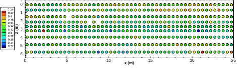
Fig. 2. A location map of measured saturated water content data
(h=0 cm) at the Las Cruces Trench site. The vertical axis represents
the depth from the surface.
2 Materials and methods
2.1 Water retention data and models
The soil hydraulic data set (i.e., water retention curves) used in this study is available through the Las Cruces Trench Site database (Wierenga et al., 1989). The database was gen-erated as part of a comprehensive field study conducted in southern New Mexico, near Las Cruces, for validating and testing numerical models of water flow and solute transport in the unsaturated zone (Wierenga et al., 1991). A 24.6-m long by 6.0-m deep trench wall was excavated, and a to-tal of 450 undisturbed samples, 7.6 cm internal diameter and 7.6 cm long, were taken from nine layers, 50 samples were taken from each layer, for every 0.5 m. Soil samples (undis-turbed and dis(undis-turbed) were then analyzed in the laboratory for soil properties, such as bulk density, saturated hydraulic conductivity, and soil water retention curve. Soil water re-tention curves were determined at 448 sampling locations, ui
(i=1, 2. . . 448) (Fig. 2). At each location, the water contents,
θ ui;hj, were measured at eleven pressure heads,hj(j=1,
2. . . 11) of 0, −10, −20, −40, −80, −120, −200, −300,
−1000, −5000, and −15 000 cm H2O. While undisturbed
soil cores were used for the wet range (−300 cm to 0 cm), disturbed soil samples were used with a standard pressure plate apparatus for the dry range (−15 000 cm to−1000 cm). More details regarding the experimental procedures can be found in Wierenga et al. (1989). The soil characterization and infiltration experiments at this site have been analyzed in a number of studies, including recent articles by Rockhold et al. (1996), Oliveira et al. (2006), and Twarakavi et al. (2008). Figure 2 shows the location map of measured saturated water contents when the pressure head is equal to 0 cm orh1
at the site. The saturated water content data are, as expected, spatially heterogeneous with mean, maximum, and minimum values of 0.322, 0.529, and 0.218, respectively. Although not shown here, water contents measured for other pressure heads are also spatially heterogeneous. Figure 3 shows sam-ple histograms of water contents for eleven pressure heads. The mean of each distribution decreases as the pressure head decreases, as expected. Not all histograms show highly skewed or asymmetric distributions, indicating that no data transformation is required. Figure 4 depicts the experimental
Table 1. Water retention,Se, models used in this study.
Models Expression Parameters
Brooks and Corey (BC) Se(h)=
( 1 h≤h
b
h
hb
−λ
h>hb
hb[cm]
λ[–]
van Genuchten (VG) Se(h)=[1+|αh1|n]m n[–]
α[cm−1] m(=1−1/n) [–]
Kosugi (KSG) Se(h)=12erfc
nln(h/ h
l) √
2σ
o
hl[cm]
σ[–]
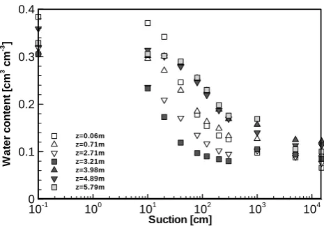
water retention curves obtained for seven different depths (z) atx=10.75 m. There are some discontinuities between the water contents observed for pressure heads of−300 cm, and those observed for−1000 cm, where water contents increase as pressure heads decrease. This is likely due to the different measurement procedures used; undisturbed soil cores were used for water content measurements from−10 to−300 cm pressure heads, while disturbed soil cores were used for pres-sure heads ranging from−1000 to−15 000 cm (Hills et al., 1993). Such inconsistency should have an impact on the re-sults of model fitting, as all data are equally weighted. Inves-tigating the impacts of this inconsistency on final parameter estimates by FI and IF approaches requires rigorous analysis of how errors are propagated between different approaches. Not surprisingly, all seven curves are quite different. Al-though this variation in the vertical direction is expected to be much more pronounced than in the horizontal direction, variations in the horizontal direction also exist and cannot be ignored, as can been seen from Fig. 2. This confirms the importance of analyzing the spatial distribution of water re-tention curves at this site.
Among many available retention curve models, the Brooks and Corey (BC) model (Brooks and Corey, 1964), the van Genuchten (VG) model (van Genuchten, 1980), and the Ko-sugi (KSG) model based on the lognormal pore size distribu-tion (Kosugi, 1996) are the most widely used analytical ex-pressions for representing the dependence of the water con-tent on the capillary pressure head for unimodal pore sys-tems. Detailed discussions of the commonly used soil hy-draulic models can be found in Leij et al. (1997). Analyti-cal expressions of the three closed-form models used in this study are listed in Table 1. The parameterSeis an effective
saturation defined as follows:
Se(h)=
θ−θr
θs−θr
(1)
whereθsandθrare the saturated and residual water contents
(m3m−3), respectively. As can be seen from Table 1, in addi-tion toθsandθr, all three models require two other shape (or
[image:3.595.310.544.87.207.2]456 H. Saito et al.: Spatial interpolation of water retention parameters 26 1 2 3 4 5 6 7 8 9 10 11 12 13 14 15 16 17 18 Figure 3: 19 20 Frequency 10 cm
.100 .200 .300 .400 .500 .000 .050 .100 .150 .200 h=-10cm
Number of Data 350 number trimmed 98
mean .29 std. dev. .04 maximum .42 median .29 minimum .10
Frequency
20 cm
.100 .200 .300 .400 .000 .040 .080 .120 .160 h=-20cm
Number of Data 448 mean .27 std. dev. .04 maximum .41 median .27 minimum .07
Frequency
15000 cm
.000 .040 .080 .120 .160 .000
.040 .080 .120
h=-15000cm
Number of Data 447 number trimmed 1
mean .09 std. dev. .02 maximum .15 median .09 minimum .03
Frequency
40 cm
.000 .100 .200 .300 .400 .000 .050 .100 .150 .200 h=-40cm
Number of Data 448 mean .23 std. dev. .05 maximum .39 median .24 minimum .05
Frequency
80 cm
.000 .100 .200 .300 .000
.040 .080 .120
h=-80cm
Number of Data 448 mean .19 std. dev. .05 maximum .36 median .19 minimum .05
Frequency
120 cm .000 .100 .200 .300 .000
.040 .080 .120
.160h=-120cm Number of Data 448
mean .17 std. dev. .05 maximum .34 median .17 minimum .05
Frequency
200 cm .000 .100 .200 .300 .000
.040 .080 .120
h=-200cm
Number of Data 448 mean .15 std. dev. .04 maximum .32 median .15 minimum .04
Frequency
300 cm .000 .050 .100 .150 .200 .250 .000
.040 .080 .120
h=-300cm
Number of Data 448 mean .14 std. dev. .04 maximum .31 median .14 minimum .04
Frequency
1000 cm .000 .050 .100 .150 .200 .000 .040 .080 .120 .160 h=-1000cm
Number of Data 447 number trimmed 1
mean .12 std. dev. .03 maximum .21 median .12 minimum .05
Frequency
5000 cm .000 .050 .100 .150 .200 .000 .050 .100 .150 .200 h=-5000cm
Number of Data 447 number trimmed 1
mean .10 std. dev. .02 maximum .17 median .10 minimum .04
Frequency
0 cm
.200 .300 .400 .500 .000
.050 .100 .150
.200h=0cm Number of Data 448
mean .32 std. dev. .03 maximum .53 median .32 minimum .22
Frequency
10 cm
.100 .200 .300 .400 .500 .000 .050 .100 .150 .200 h=-10cm
Number of Data 350 number trimmed 98
mean .29 std. dev. .04 maximum .42 median .29 minimum .10
Frequency
20 cm
.100 .200 .300 .400 .000 .040 .080 .120 .160 h=-20cm
Number of Data 448 mean .27 std. dev. .04 maximum .41 median .27 minimum .07
Frequency
15000 cm
.000 .040 .080 .120 .160 .000
.040 .080 .120
h=-15000cm
Number of Data 447 number trimmed 1
mean .09 std. dev. .02 maximum .15 median .09 minimum .03
Frequency
40 cm
.000 .100 .200 .300 .400 .000 .050 .100 .150 .200 h=-40cm
Number of Data 448 mean .23 std. dev. .05 maximum .39 median .24 minimum .05
Frequency
80 cm
.000 .100 .200 .300 .000
.040 .080 .120
h=-80cm
Number of Data 448 mean .19 std. dev. .05 maximum .36 median .19 minimum .05
Frequency
120 cm .000 .100 .200 .300 .000
.040 .080 .120
.160h=-120cm Number of Data 448
mean .17 std. dev. .05 maximum .34 median .17 minimum .05
Frequency
200 cm .000 .100 .200 .300 .000
.040 .080 .120
h=-200cm
Number of Data 448 mean .15 std. dev. .04 maximum .32 median .15 minimum .04
Frequency
300 cm .000 .050 .100 .150 .200 .250 .000
.040 .080 .120
h=-300cm
Number of Data 448 mean .14 std. dev. .04 maximum .31 median .14 minimum .04
Frequency
1000 cm .000 .050 .100 .150 .200 .000 .040 .080 .120 .160 h=-1000cm
Number of Data 447 number trimmed 1
mean .12 std. dev. .03 maximum .21 median .12 minimum .05
Frequency
5000 cm .000 .050 .100 .150 .200 .000 .050 .100 .150 .200 h=-5000cm
Number of Data 447 number trimmed 1
mean .10 std. dev. .02 maximum .17 median .10 minimum .04
Frequency
0 cm
.200 .300 .400 .500 .000
.050 .100 .150
.200h=0cm Number of Data 448
mean .32 std. dev. .03 maximum .53 median .32 minimum .22
Fig. 3. Sample histograms of water contents for eleven pressure heads (sequentially,h=0,−10,−20,−40,−80,−120,−200,−300,−1000,
−5000, and−15 000 cm).
empirical) parameters, leading to a total of four parameters representing the retention curve models.
Application of these water retention functions requires re-liable estimates of the parameters for a soil of interest. While
θs can be obtained independently, the other retention
pa-rameters usually have to be estimated indirectly, by fitting the analytical function to the experimental water retention data using an optimization approach, such as a non-linear least-squares minimization approach (e.g., implemented in the RETC code). In most optimization procedures, perfor-mance is improved if the initial estimates are close to the “true” solution. In other words, if initial estimates are too far from the “true” solutions, the solution may not converge to the global minimum, but to the local minimum during the optimization process. Seki (2007) recently developed a pro-gram code that uses a full-automatic procedure to estimate soil water retention model parameters. The program auto-matically selects initial estimates based on observations, so that the user does not have to make his/her selections.
De-27 1 2 3 4 5 6 7 8 9 10 11 Figure 4: 12 Suction [cm] W a te r c o n te n t [c m 3 cm -3 ]
10-1 100 101 102 103 104
[image:4.595.311.544.504.666.2]0 0.1 0.2 0.3 0.4 z=0.06m z=0.71m z=2.71m z=3.21m z=3.98m z=4.89m z=5.79m
Fig. 4. Water retention curves obtained for seven different depths at
x=10.75 m.
H. Saito et al.: Spatial interpolation of water retention parameters 457 28 1 2 3 4 5 6 7 8 9 10 11 12 13 14 15 16 17 18 Figure 5: 19 20 Frequency sigmal .00 1.00 2.00 3.00 .000
.040 .080 .120
LN model: sigma
Number of Data 448 mean 1.58 std. dev. .54 maximum 5.78
median 1.51 minimum .65
Frequency
alphav .000 .050 .100 .150 .200 .000
.050 .100 .150
.200VG model: alpha Number of Data 448
mean .12 std. dev. 1.34 maximum 28.16
median .04 minimum .00
Frequency
hb
.0 10.0 20.0 30.0 40.0 50.0 .000 .050 .100 .150 .200 .250
BC model: h
Number of Data 448 mean 15.04 std. dev. 8.59 maximum 64.46
median 14.68 minimum .04
Frequency
hl
0. 100. 200. 300. .000
.040 .080 .120 .160
LN model: h
Number of Data 448 mean 87.57 std. dev. 76.22 maximum 816.49
median 64.97 minimum .61
Frequency
lambdab .00 .50 1.00 1.50 2.00 .000
.040 .080 .120 .160
BC model: lambda
Number of Data 448 mean .46 std. dev. .25 maximum 1.77
median .41 minimum .11
Frequency
nv
1.00 2.00 3.00 4.00 .000
.050 .100 .150 .200
VG model: n
Number of Data 448 mean 1.71 std. dev. .36 maximum 3.60
median 1.64 minimum 1.14
Frequency
qrb
.000 .050 .100 .150 .200 .000
.040 .080 .120
.160BC model: q_r Number of Data 448
mean .06 std. dev. .03 maximum .14 median .06 minimum .00
Frequency
qrl
.000 .050 .100 .150 .200 .000
.050 .100 .150 .200
LN model: q_r
Number of Data 448 mean .09 std. dev. .02 maximum .16 median .09 minimum .01
Frequency
qrv
.000 .050 .100 .150 .200 .000
.050 .100 .150 .200
VG model: q_r
Number of Data 448 mean .08 std. dev. .03 maximum .15 median .08 minimum .00
Frequency
qsb
.200 .300 .400 .500 .000
.050 .100 .150
.200BC model: q_s Number of Data 448
mean .32 std. dev. .03 maximum .51 median .31 minimum .22
Frequency
qsl
.200 .300 .400 .500 .000
.040 .080 .120 .160
LN model: q_s
Number of Data 448 mean .32 std. dev. .03 maximum .51 median .32 minimum .22
Frequency
qsv
.200 .300 .400 .500 .000
.040 .080 .120 .160
VG model: q_s
Number of Data 448 mean .32 std. dev. .03 maximum .47 median .32 minimum .22
Frequency
sigmal .00 1.00 2.00 3.00 .000
.040 .080 .120
LN model: sigma
Number of Data 448 mean 1.58 std. dev. .54 maximum 5.78
median 1.51 minimum .65
Frequency
alphav .000 .050 .100 .150 .200 .000
.050 .100 .150
.200VG model: alpha Number of Data 448
mean .12 std. dev. 1.34 maximum 28.16
median .04 minimum .00
Frequency
hb
.0 10.0 20.0 30.0 40.0 50.0 .000 .050 .100 .150 .200 .250
BC model: h
Number of Data 448 mean 15.04 std. dev. 8.59 maximum 64.46
median 14.68 minimum .04
Frequency
hl
0. 100. 200. 300. .000
.040 .080 .120 .160
LN model: h
Number of Data 448 mean 87.57 std. dev. 76.22 maximum 816.49
median 64.97 minimum .61
Frequency
lambdab .00 .50 1.00 1.50 2.00 .000
.040 .080 .120 .160
BC model: lambda
Number of Data 448 mean .46 std. dev. .25 maximum 1.77
median .41 minimum .11
Frequency
nv
1.00 2.00 3.00 4.00 .000
.050 .100 .150 .200
VG model: n
Number of Data 448 mean 1.71 std. dev. .36 maximum 3.60
median 1.64 minimum 1.14
Frequency
qrb
.000 .050 .100 .150 .200 .000
.040 .080 .120
.160BC model: q_r Number of Data 448
mean .06 std. dev. .03 maximum .14 median .06 minimum .00
Frequency
qrl
.000 .050 .100 .150 .200 .000
.050 .100 .150 .200
LN model: q_r
Number of Data 448 mean .09 std. dev. .02 maximum .16 median .09 minimum .01
Frequency
qrv
.000 .050 .100 .150 .200 .000
.050 .100 .150 .200
VG model: q_r
Number of Data 448 mean .08 std. dev. .03 maximum .15 median .08 minimum .00
Frequency
qsb
.200 .300 .400 .500 .000
.050 .100 .150
.200BC model: q_s Number of Data 448
mean .32 std. dev. .03 maximum .51 median .31 minimum .22
Frequency
qsl
.200 .300 .400 .500 .000
.040 .080 .120 .160
LN model: q_s
Number of Data 448 mean .32 std. dev. .03 maximum .51 median .32 minimum .22
Frequency
qsv
.200 .300 .400 .500 .000
.040 .080 .120 .160
VG model: q_s
[image:5.595.112.478.65.425.2]Number of Data 448 mean .32 std. dev. .03 maximum .47 median .32 minimum .22
Fig. 5. Sample histograms of water retention curve model parameters for BC (left), VG (middle), and KSG (right) models. The saturated
and residual water contents are in the top two rows, two shape parameters are in the bottom two rows.
tails of this approach will not be discussed in this paper, but it should be noted that the full-automatic approach worked very well in most cases when applied to a number of water retention data from the UNSODA database (Leij et al., 1996). Such an approach is especially attractive when a great num-ber of retention curves need to be fitted simultaneously. All three models were fitted to 448 retention data points using the full-automatic procedure to obtain water retention param-eters at all sampling locations. Figure 5 shows histograms of retention parameters, includingθs andθr. Similar to the
wa-ter content histograms shown in Fig. 3,θs andθr histograms
show no significant skewness and are more-or-less symmet-ric, except forθr of the BC and VG models, where about
12 and 2.5% of data have a value of 0, respectively. As for the shape parameters (e.g., αv andnv), most are positively
skewed. The parameterhb even shows a bimodal
distribu-tion.
2.2 Geostatistical interpolation theory
To estimate an unknown value of a given soil property at un-sampled locations, a geostatistical least-square interpolation technique, known as kriging, was used in this study. Con-sider the problem of estimating the value of a soil attribute
z(e.g., water content or soil hydraulic parameters) at an un-sampled location u, where u is a vector of spatial coordinates. The available information consists of values of the variable
zatN locations ui,i=1, 2. . .N. All univariate kriging
esti-mates are variants of the general regression estimatez∗(u) defined as:
z∗(u)−m (u)=
n(u)
X
α=1
λα(u)[z (uα)−m (uα)] (2)
where λα(u) is the weight assigned to datum z(uα) and m(u) is the trend component of the spatially varying at-tribute (Goovaerts, 1997). In practice, only those observa-tions closest to u are retained, that is then(u) data within a
458 H. Saito et al.: Spatial interpolation of water retention parameters given neighborhood or windowW(u) centered on u, while
the influence of those farther away are discarded (Saito and Goovaerts, 2000). One of the most common kriging estima-tors is ordinary kriging (or OK), which estimates an unknown value as a linear combination of neighboring observations:
z∗(u)=
n(u)
X
α=1
λOKα (u) z (uα) (3)
In OK, unlike the constant value used in simple kriging, the mean (or trend) at each estimation location (i.e., local mean,m(u)) is implicitly re-estimated. OK weightsλOKα are determined so as to minimize the error or estimation vari-anceσ2(u)= Var{Z∗(u)−Z(u)}under the constraint of an unbiased estimate (Goovaerts, 1997). These weights are ob-tained by solving the system of linear equations known as the ordinary kriging system:
n(u)
P
β=1
λOKβ (u) γ (uα−uβ)+µOK(u)=γ (uα−u) α=1, ..., n(u)
n(u)
P
β=1
λOKβ (u)=1
(4)
whereµOK(u) is the Lagrange parameter, γ(uα-uβ) is the
semivariogram between observations at uα and uβ, and γ(uα-u) is the semivariogram between the datum location
uα and the location being estimated, u. The semivariogram γ(h) models the variability between observations separated by a vector h. The only information required by the system (Eq. 4) are the semivariogram values,γ, for different sepa-ration distances. These values are readily derived from the semivariogram model fitted to experimental values (i.e., lin-ear model of regionalization):
ˆ
γ (u)= 1
2N (h) n(u)
X
α=1
[z (uα)−z (uα+h)]2 (5)
whereN(h) is the number of data pairs for a given separa-tion vector h. The choice of the model is limited to funcsepara-tions that ensure a positive definite covariance function matrix of the left-hand-side of the kriging system (Eq. 4). Spatial cor-relations often vary with direction, and such a case requires one to compute semivariograms in different orientations to fit anisotropic (direction-dependent) semivariogram models. In this study, differences in horizontal and vertical variations observed in retention data were taken into account by con-sidering anisotropic semivariograms. Details of model fit-ting can be found in Deutsch and Journel (1998), Goovaerts (1997), and Kitanidis (1997). In addition to an estimate of the unknown z value, OK provides an error variance that is computed as
σOK2 (u)=
n(u)
X
α=1
λα(u) γ (uα−u)−µ (u) (6)
When histograms show positively skewed distributions and/or are not unimodal, OK might not be the best ap-proach to estimate values at unsampled locations (Saito and
Goovaerts, 2000). In such case, indicator kriging (IK), in which all data are transformed into either 0 or 1 depending upon the exceedence of a given threshold (Journel, 1983), can be used. Indicator kriging allows one to estimate the probabilities of exceeding a series of thresholds at unsam-pled locations, leading to the construction of conditional cu-mulative distribution functions (ccdf) of the variable of inter-est. Once the ccdf is obtained, an optimal estimate and the uncertainty associated with the estimated value can be quan-tified by taking the mean (E-type estimate) and variance of the ccdf, respectively.
The conditional probabilities at u for a series of thresh-oldszk discretizing a range of variation ofzare estimated as
a linear combination ofn(u) surrounding indicator transfor-mation of datai(uα;zk):
[F (u;zk|(n))]∗=[Pr{Z (u)≤zk|(n)}]∗=
n(u)
X
α=1
λα(u) i (uα;zk) (7)
where
i (uα;zk)=
1 ifz (uα)≤zk
0 otherwise k=1, ..., K (8) Kriging weights λα(u; zk) are then computed from the
in-dicator kriging system, similar to the OK system (Eq. 4), where all experimental semivariogramsγ(u) are replaced by indicator semivariogramsγI(u). A major drawback of IK is
that in order to construct ccdfs at any location u,Kindicator semivariograms, usually 9 to 16 (Deutsch and Journel, 1998), have to be computed, andKindicator kriging systems have to be solved. Consequently, IK is much more computation-ally demanding than OK. It is common to use nine deciles of the sample distribution as thresholds. More details on indi-cator kriging can be found in Goovaerts (1999).
2.3 Prediction performances: FI vs. IF
To compare the FI and IF approaches in terms of reproduc-tion of WRC atilocations ui,Se(h; ui), two standard
valida-tion techniques were used: a leave-one-out cross-validavalida-tion, in which one observation at a time is temporarily removed from the dataset and re-estimated from remaining data, and a split-sample method, where the dataset is divided into two non-overlapping observation and validation sets (Fig. 6). The number of observation locations in each set were 199 (Np)
and 249 (Nv), respectively. In the split-sample method, the
observation set was used to estimate values at all locations in the validation set so that estimation errors could be calculated explicitly. Figure 6 depicts the location map of both obser-vation and validation sets used in the split-sample method. For complete full validation, different split scenarios had to be tried. In this study, only the scenario shown in Fig. 6 was used. This scenario was considered because it is the most likely and realistic scenario where samples were taken layer-by-layer, but not randomly. In addition, the main purpose of using the split-sample method was to investigate the impact
H. Saito et al.: Spatial interpolation of water retention parameters 459
29 1
2
3
4
5
6
Figure 6:
7
8
x (m)
z(
m
)
0 5 10 15 20 25
0
1
2
3
4
5
6
Sample set Validation set
Fig. 6. Locations used for sample (closed squares) and validation
(open squares) sets in the split-sample procedure.
of the sample size. Note that, in this study, the ogram models used in kriging were those fitted to semivari-ograms for all 448 observations. Details about the FI and IF approaches used in the study are given below.
2.3.1 FI approach
1. Parameters for three water retention functions (BC, VG, and KSG) were first obtained for all 448 water retention curvesSe(h; ui) using the automatic fitting procedure
(Seki, 2007).
2. For each soil hydraulic parameter, unknown values were estimated at all 448 locations for the leave-one-out cross-validation, and at 249 locations for the split-sample method. Following two interpolation ap-proaches were compared:
(a) Ordinary kriging (OK) was used for all parameters.
(b) While OK was used for θs and θr,
indicator kriging (IK) was used for the shape parameters.
The former is referred to as the FIOK approach, while
the latter will called the FIIKapproach for the remainder
of the paper.
3. For each model and approach, a discrepancy between observed water retention curvesSe(h; ui) and those
cal-culated from estimated parameters Se(h; ui) was
ob-tained at each location by computing differences in wa-ter contents at the eleven corresponding pressure heads. Mean absolute error (MAE) and mean error (bias ME) are used in this study in the following way:
MAE= 1 N
N
X
i=i
"
1 11
11
X
j=1
ˆ
θ ui;hj−θ ui;hj
#
(9)
ME= 1 N
N
X
i=i
"
1 11
11
X
j=1
ˆ
θ ui;hj−θ ui;hj
#
(10)
whereN is 448 for the leave-one-out cross-validation and 249 for the split-sample method, θˆ ui;hj
is the water content at the location ui calculated from
estimated parameters for the pressure head hj, and θ ui;hjis the observed water content at the location
ui for the pressure headhj.
2.3.2 IF approach
1. Unknown water content values corresponding to eleven pressure heads were estimated using OK at 448 loca-tions for the leave-one-out cross-validation and 249 lo-cations for the split-sample method.
2. Using the automatic fitting procedure (Seki, 2007), pa-rameters for three WRC models (i.e., BC, VG, and KSG) were obtained at each estimated location. To ac-count for estimation errors when fitting retention mod-els, eachh-θpair was weighted based on the reciprocal of the kriging variance after all kriging variances were standardized by the total sills of the semivariograms. More weights are therefore given to those data points for which the error variances were small.
3. For each model, the discrepancy between observed wa-ter retention curves and those calculated from parame-ters obtained in the previous step was obtained by com-puting MAE and ME, similar to what was done for the FI approach.
4. The impact of the number of data pairs used to con-struct WRC when estimating parameters was investi-gated by repeating 1 through 3, using only the follow-ing six pressure heads: 0,−20,−80,−200,−1000, and
−15 000 cm. This approach is referred to as IF6 in the remainder of the paper, while the approach considering all eleven pressure heads is referred to as IF11. The number of data pairs used in the IF approach is arbi-trary. The optimum number depends on many factors, including soil type. In this study, instead of finding the optimum number of data pairs for this particular data set, we have investigated how prediction errors change when the number of data pairs is reduced to about half of the original number.
3 Results and discussions
The results are divided into two sections. The first section summarizes experimental semivariograms computed from water retention data and model parameters. In the second section, different approaches (IF and FI) are compared in terms of describing the spatial distribution of soil hydraulic parameters.
[image:7.595.52.283.64.127.2]3.1 Semivariograms
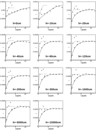
Figure 7 shows the experimental semivariograms of WRC model parameters with fitted geometric anisotropy models. Semivariograms of water contents corresponding to eleven
460 H. Saito et al.: Spatial interpolation of water retention parameters
30 1
2
3
4
5
6
7
8
9
10
11
12
13
14
15
16
17
18
19
20
21
Figure 7:
22
Lag [m]
γ
0 5 10
0 0.0005 0.001 0.0015
θsb
Lag [m]
γ
0 5 10
0 0.0007 0.0014 0.0021
θsv
Lag [m]
γ
0 5 10
0 0.0005 0.001 0.0015
θsl
Lag [m]
γ
0 5 10
0 0.0005 0.001 0.0015
θrb
Lag [m]
γ
0 5 10
0 0.0003 0.0006 0.0009
θrv
Lag [m]
γ
0 5 10
0 0.0002 0.0004 0.0006
θrl
Lag [m]
γ
0 5 10
0 30 60 90
hb
Lag [m]
γ
0 5 10
0 1.5 3 4.5
αv
Lag [m]
γ
0 5 10
0 2400 4800 7200
hl
Lag [m]
γ
0 5 10
0 0.03 0.06 0.09
λb
Lag [m]
γ
0 5 10
0 0.06 0.12 0.18
nv
Lag [m]
γ
0 5 10
0 0.13 0.26 0.39
[image:8.595.130.468.61.513.2]σl
Fig. 7. Experimental semivariograms of water retention curve model parameters with fitted geometric anisotropy models for horizontal
(circles and the solid line) and vertical (triangles and the dashed line) directions. Semivariograms were calculated from model parameters at
448 sampling locations. Subscriptsb,v, andlcorrespond to BC (the left column), VG (the middle column), and KSG (the right column)
models, respectively.
pressure heads, h1−h11, with fitted geometric anisotropy models are depicted in Fig. 8. All these semivariograms were calculated using 448 observations. Except forαv, there
is clear anisotropy in all semivariograms with major spa-tial continuity observed in the horizontal direction. While horizontal semivariograms, are generally well structured, in most cases vertical semivariograms fluctuate a lot and are not smooth. There are not a sufficient number of pairs in the ver-tical direction to obtain well structured semivariograms. Ex-istence of soil horizons would also not result in spatial cor-relation of soil variables in the vertical direction at the scale
of observations. All experimental horizontal semivariograms were fitted using either exponential or spherical models, and they all display a clear nugget effect. Ranges and sill values vary depending on the variable. For example, as expected, semivariograms for the saturated (θs) and residual (θr)
volu-metric water contents are similar for all three models (Fig. 7, top two rows). However, other parameters have semivari-ograms of different shapes, which was expected as the spatial distribution of these parameters varies. Geometric anisotropy models, in which the same nugget and sill values are used for different directions, were fitted for vertical semivariograms.
H. Saito et al.: Spatial interpolation of water retention parameters 461
31 1
2
3
4
5
6
7
8
9
10
11
12
13
14
15
16
17
18
19
Figure 8:
20
Lag [m]
γ
0 5 10
0 0.0005 0.001 0.0015
h=0cm
Lag [m]
γ
0 5 10
0 0.0007 0.0014 0.0021
h=-10cm
Lag [m]
γ
0 5 10
0 0.001 0.002 0.003
h=-20cm
Lag [m]
γ
0 5 10
0 0.0012 0.0024 0.0036
h=-40cm
Lag [m]
γ
0 5 10
0 0.0012 0.0024 0.0036
h=-80cm
Lag [m]
γ
0 5 10
0 0.001 0.002 0.003
h=-120cm
Lag [m]
γ
0 5 10
0 0.0008 0.0016 0.0024
h=-200cm
Lag [m]
γ
0 5 10
0 0.0006 0.0012 0.0018
h=-300cm
Lag [m]
γ
0 5 10
0 0.0004 0.0008 0.0012
h=-1000cm
Lag [m]
γ
0 5 10
0 0.0002 0.0004 0.0006
h=-5000cm
Lag [m]
γ
0 5 10
0 0.0002 0.0004 0.0006
h=-15000cm
Fig. 8. Experimental semivariograms of water retention data (water contents for a particular pressure head) with fitted geometric anisotropy
models for horizontal (circles and the solid line) and vertical (triangles and the dashed line) directions. Semivariograms were calculated from retention data obtained at 448 sampling locations.
Nugget effects may be underestimated using this approach, since the number of data pairs in the vertical direction is not sufficient. Using a geometric anisotropy model instead of a zonal anisotropy model, which can be used to account for difference in spatial correlation between vertical and hori-zontal directions, is justified and needed since kriging sys-tems requires the same nugget effect in different directions (Gringarten and Deutsch, 2001). In practice, unless there are conclusive physical explanations for phenomena, it is com-mon to use geometric anisotropy models.
As for the semivariograms of water contents at particu-lar pressure heads (Fig. 8), the ranges of water contents near saturation in the horizontal direction (i.e., a major range) are generally larger than those for drier conditions. This sug-gests that the spatial continuity of larger pores is more pro-found than that of smaller pores. When pressure heads are smaller than−40 cm, the shape of the semivariograms be-comes almost identical. From the Laplace equation for cap-illary rise, the radius of a pore corresponding to a pressure head of−40 cm can be calculated to be about 0.035 mm (as-suming that the contact angle is equal to 0◦). Therefore, it can
[image:9.595.129.466.61.514.2]462 H. Saito et al.: Spatial interpolation of water retention parameters
32 1
2
3
4
5
6
7
8
9
10
Figure 9: 11
Suction [cm]
W
a
te
r
c
ont
e
n
t
(c
m
3
cm
-3 )
10-1 100 101 102 103 104
0 0.1 0.2 0.3 0.4
Fit FIOKKSG
[image:10.595.50.287.62.201.2]IF11 KSG Observations Kriged WRC
Fig. 9. Water retention data observed (square), fitted using the KSG
model (solid black line), and kriged (triangle) at (x, y)=(7.25, 2.16). In the IF approach, the KSG model was fitted to the constructed wa-ter retention curve (red). In the FI approach, KSG model paramewa-ters were kriged using ordinary kriging to obtain the FI-KSG curve.
33 1
2
3
4
5
6
7
Figure 10: 8
9
10 0.00 0.01 0.02 0.03 0.04 0.05
BC VG KSG
Model
MA
E
FI_OK FI_IK IF11 IF6
0.00 0.01 0.02 0.03 0.04 0.05
BC VG KSG
Model
MA
E
(a) (b)
0.00 0.01 0.02 0.03 0.04 0.05
BC VG KSG
Model
MA
E
FI_OK FI_IK IF11 IF6
0.00 0.01 0.02 0.03 0.04 0.05
BC VG KSG
Model
MA
E
(a) (b)
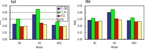
Fig. 10. The impact of the choice of the approach on mean
abso-lute errors (MAE) of retention curve predictions for (a) the leave-one-out cross-validation and (b) the split-sample procedures. Three WRC models (BC, VG, and KSG) were compared.
be expected that spatial distributions of pores smaller than 0.035 mm are similar in this soil.
3.2 Prediction performance
Using both the FI and IF approaches, water retention curve model parameters can be obtained at any location. Figure 9 shows differences between the FI and IF approaches in esti-mating a water retention curve using the KSG model at a se-lected location, (x,z)=(7.25, 2.16), where observed retention data (squares) are available. Due to the exactitude property of kriging, data at this location were not included in krig-ing (i.e., the leave-one-out cross-validation). While the blue line is obtained with parameters predicted by the FIOK
ap-proach, the red line is calculated with parameters obtained by the IF11 approach. In the FIOK approach, model
param-eters were estimated directly from surrounding conditioning parameters using OK. In the IF11 approach, the water reten-tion curve was first constructed by interpolating water con-tent values corresponding to eleven pressure heads,h1−h11.
Constructed water retention data are shown in Fig. 9 using red symbols. The KSG model (the solid red line in Fig. 9) was then fitted to the constructed retention data using the
34 1
2
3
4
5
6
7
8
9
Figure 11:
10
11
Suction [cm]
W
a
te
r
C
onte
n
t
[m
3 /m -3 ]
10-3 10-2 10-1 100 101 102 103 104 0
0.1 0.2 0.3 0.4
Fit (VG model) Observations
[image:10.595.310.545.65.223.2](x, y) = (12.75, 3.21)
Fig. 11. Observed water retention data (square) with the VG model
fitted at (x, y)=(12.75, 3.21).
aforementioned non-linear least squared method to obtain model parameters. While the model obtained using the FIOK
approach could not reproduce theS-shape trend observed in retention data well, the IF11 approach could capture the trend of WRC reasonably well. This confirms that, depending on the chosen approach, resulting WRC models can be signif-icantly different. In the following section, both approaches were compared in a more comprehensive manner using the leave-one-out cross-validation and the split-sample methods. Figure 10 depicts the mean absolute prediction errors (MAE) calculated for all four approaches, i.e., FIOK, FIIK,
IF11, and IF6, using the leave-one-out cross-validation and the split-sample procedures for the three WRC models. In general, both IF approaches resulted in smaller MAE than the FI approaches, regardless of which WRC model was used. Decreases in prediction errors were much larger when the VG model was used, mainly because the prediction per-formance of the VG model for the FI approach was much worse than that for the other two models. At one location, (x,z)=(12.75, 3.21), the fitted parameterαv(=28.16 cm−1)
was three orders of magnitude greater than in the rest of the domain, where the mean of fitted αv is 0.12 cm−1 and the
median is 0.04 cm−1 (see the histogram of αv in Fig. 5).
Although the fit was acceptable at this particular location (Fig. 11), the large αv value (an outlier) affected the
esti-mation ofαv values at surrounding locations, leading to a
relatively poor performance of the FIOKapproach for the VG
model. Indicator kriging was expected to reduce the impact of outliers in the FI approach, as all data are transformed first to binary data, either 0 or 1, depending upon exceedence of the threshold value. However, whenE-type estimates were computed, the observed extreme value was taken as a possi-ble maximum value. Because of that, the indicator approach could not improve the prediction. The problem associated with the outlier can be avoided if the IF approach is used. For the other two WRC models, BC and KSG, average predic-tion errors decreased by about 10–15% when the IF approach
[image:10.595.52.287.287.367.2]H. Saito et al.: Spatial interpolation of water retention parameters 463
35 1
2
3
4
5
6
7
Figure 12: 8
-0.01 0.00 0.01 0.02 0.03 0.04
BC VG KSG
Model
ME
FI_OK FI_IK IF11 IF6
-0.02 -0.01 0.00 0.01 0.02 0.03 0.04
BC VG KSG
Model
ME
(a) (b)
-0.01 0.00 0.01 0.02 0.03 0.04
BC VG KSG
Model
ME
FI_OK FI_IK IF11 IF6
-0.02 -0.01 0.00 0.01 0.02 0.03 0.04
BC VG KSG
Model
ME
(a) (b)
Fig. 12. The impact of the choice of the approach on mean errors
(ME) of retention curve predictions for (a) the leave-one-out cross-validation and (b) the split-sample procedure. Three WRC models (BC, VG, and KSG) were compared.
was used in comparison with the prediction errors for the FI approach, where there were no obvious outliers in initially evaluated parameters.
For the FIOKapproach, mean absolute errors vary
depend-ing on the WRC model used. On the other hand, predic-tion errors do not depend upon the model used for the IF approach. This is not a surprising result since three models were fitted to the same reconstructed WRCs in the IF ap-proach. Therefore, the prediction errors calculated for the IF approach are mainly the summary of model fitting perfor-mance, but do not directly reflect the accuracy of interpola-tion as those for the FI approach do.
With regard to MAE, there is no distinct trend in whether the IF11 approach is better than the IF6 approach is bet-ter. While IF6 outperforms IF11 when the VG model was used for both the leave-one-out cross validation and the split-sample method, IF11 had slightly smaller mean absolute er-rors or almost the same erer-rors when compared to IF6 for the BC and KSG models. This indicates that reducing the num-ber ofθ-hpairs by about half does not necessarily worsen prediction performances, at least for this particular data set, as long as the IF approach is adopted. This result is quite im-portant, since the main reason for preferring the FI approach over the IF approach in most studies is that the number of variables one needs to analyze can be significantly reduced. The number of parameters required in the WRC models used in this study is four, which is significantly smaller than the original elevenθ-h pairs used to construct water retention curves. To use all pairs in the IF approach, one needs to per-form kriging eleven times, which requires significantly more effort than performing it only four times in the FI approach. However, it was just shown here that when the number of data pairs is reduced to six, the IF approach is still better than the FI approach. With a little extra work, we can im-prove the description of the spatial distribution of water re-tention curves using the IF approach. This may not be true when soils with multimodal pore systems (e.g., aggregated soils) are considered. Such soils may require models that can distinguish between different pore systems, such as the Durner model (Durner, 1994). To obtain parameters for such models, we need to have moreθ-hpairs than required by tra-ditional unimodal models. An appropriate number of pairs
36 1
2
3
4
5
6
7
8
9
10
11
12
13
14
15
16
Figure 13: 17
18
19
20
x (m)
z(
m
)
0 5 10 15 20 25
0
2
4
6 (a)
x (m)
z(
m
)
0 5 10 15 20 25
0
2
4
6 (b)
x (m)
z(
m
)
0 5 10 15 20 25
[image:11.595.309.545.63.393.2]0 2 4 6 (c)
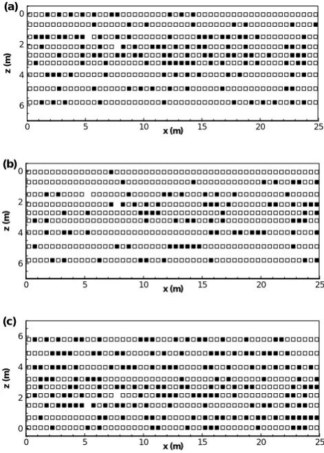
Fig. 13. Locations where IF11 outperformed FI in terms of mean
absolute errors (i.e., smaller MAE) are depicted by open squares, while closed squares indicate locations where FI outperformed IF for (a) BC, (b) VG, and (c) KSG models.
thus varies depending upon the soil type and can be assessed using the IF approach. This is another advantage of the IF approach over the FI approach.
As for the mean error, there is no obvious trend of over-or under-estimation, except fover-or the VG model where mean errors are always positive (meaning that predicted water con-tents are, on average, greater than observed values). When comparing different approaches, ME is much smaller (i.e., has less bias) for the IF approaches than for the FI ap-proaches, except when the BC model was considered in the split-sample method. Like that for MAE, this result con-firms the superiority of the IF approach over the FI approach. While for the BC and KSG models, IF11 resulted in less bias than IF6, for the VG model, IF6 had much smaller biases than IF11 for both the leave-one-out cross-validation and the split-sample method. This indicates again that reducing the number of h-θ pairs from eleven to six in the IF approach does not necessarily worsen the overall performance.
Figure 13 shows spatial distributions of locations where IF11 outperformed FIOK (open squares), and vice versa
[image:11.595.48.287.65.143.2]464 H. Saito et al.: Spatial interpolation of water retention parameters
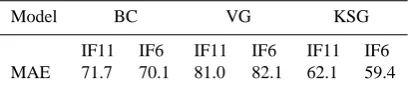
Table 2. Percentages (%) of locations where mean absolute errors
(MAE) for the IF approach were smaller than those for the FI ap-proach in the leave-one-out cross-validation.
Model BC VG KSG
IF11 IF6 IF11 IF6 IF11 IF6
MAE 71.7 70.1 81.0 82.1 62.1 59.4
(closed squares), in terms of MAE in the leave-one-out cross-validation. There is no specific trend observed, such as a cluster of open or closed squares. This means that the pre-diction of water retention curves was spatially unbiased. Pro-portions of open squares for both IF11 and IF6 (spatial dis-tributions are not shown) are summarized in Table 2 for all cases. For all models, the IF approaches outperformed the FI approaches at more than 60% of the sampling locations. For the VG model especially, the IF approaches resulted in smaller prediction errors at more than 80% of the sampling locations. Although the difference between IF11 and IF6 is small, IF11 was slightly better than IF6 for BC and KSG, while IF6 was better than IF11 for VG. Overall, these per-centages confirm the superiority of the IF approach over the FI approach in predicting WRCs at any given location.
4 Conclusions
This study compared the performance of two interpolation approaches, a commonly used fit-first interpolate-later (FI) approach and a proposed interpolate-first fit-later (IF) ap-proach, to estimate the spatial distribution of water tion curve parameters. In the former approach, the reten-tion curve model parameters are first evaluated at sampled locations from observed retention data, and then these pa-rameters are interpolated directly for locations without mea-surements. In the latter approach, retention data are first in-terpolated for locations without measurements, and then re-tention curve model parameters are fitted to these estimated retention curves. Three retention models, Brooks and Corey, van Genuchten, and Kosugi models were considered. As for spatial interpolation, a least-squared interpolation technique, known as kriging, was used. For variables that do not show asymmetric distributions, ordinary kriging was used, while for those with asymmetric distributions, indicator kriging was used as well. Standard validation techniques (the leave-one-out cross-validation and the split-sample methods) were used to compare the two approaches in terms of reproducing retention curves.
Both validation results showed that, regardless of the re-tention model selected, the IF approach had lower predic-tion errors (mean absolute errors) when compared to the FI approach. Improvements were especially substantial for the
VG model because an extreme value in initially estimated parameters led to the poor estimate of that parameter at sur-rounding locations in the FI approach. There is always a risk of including parameter outliers in the estimation process as long as the FI approach is used. In the IF approach, such a problem rarely occurs. In addition, the IF approach per-formed better than the FI approach even when the number of data pairs used to construct retention curves was reduced from eleven to six. This makes the IF approach comparable to the FI approach in terms of workload, because the number of variables used in the FI approach is four, while that in the IF approach would be only six. The FI approach has been preferred mainly because one can reduce the computational time and workload. However, as this study shows, with a little bit of extra work, one can achieve a much better estima-tion of the spatial distribuestima-tion of water retenestima-tion curves by using the IF approach. In the future, the IF approach should be applied to estimate unsaturated hydraulic conductivity as well.
Overall, this study shows the superiority of the IF approach over the FI approach in evaluating the spatial distribution of water retention curves, which is the initial but critical step in modeling variably-saturated water flow and solute transport in field-scale heterogeneous soils. This study shows that interpolating retention model parameters, suchn
andαin the VG model, should be done with extreme care. In future studies, the actual impact of the FI approach on water flow and solute transport still needs to be investigated. Edited by: W. Durner
References
Brooks, R. J. and Corey, A. T.: Hydraulic properties of porous me-dia, Hydrology Paper no. 3, Civil Engineering Department, Col-orado State Univ., Fort Collins, ColCol-orado, USA, 1964.
Burdine, N. T.: Relative permeability calculations from pore-size distribution data. Transactions of the American Institute of Min-ing, Metall. Petrol. Eng., 198, 71–77, 1957.
Deutsch, C. V. and Journel, A.: GSLIB: Geostatistical Software Library and User’s Guide, Oxford Univ. Press, New York, USA, 1998.
Durner, W.: Hydraulic conductivity estimation for soils with het-erogeneous pore structure, Water Resour. Res., 32(9), 211–223, 1994.
Hills, R. G., Wierenga, P., Luis, S., McLaughlin, D., Rockhold, M., Xiang, J., Scanlon, B. and Wittmeyer, G.: INTRAVAL – Phase II model testing at the Las Cruces Trench Site, Tech. rep., US Nu-clear Regulatory Commission – NUREG/CR-6063, Washington, DC, USA, 131 pp., 1993.
Goovaerts, P.: Geostatistics for Natural Resources Evaluation. Ox-ford Univ. Press, New York, USA, 483 pp., 1997.
Goovaerts, P.: Geostatistics in soil science: state-of-the-art and per-spectives, Geoderma, 89, 1–45, 1999.
Gringarten, E. and Deutsch, C. V.: Teacher’s Aide, Variogram In-terpretation and Modeling, Math. Geol., 33(4): 507–534, 2001.
H. Saito et al.: Spatial interpolation of water retention parameters 465
Heuvelink, G. B. M. and Pebesma, E. J.: Spatial aggregation and soil process modelling, Geoderma, 89, 47–65, 1999.
Journal, A. G.: Nonparametric estimation of spatial distributions. Math. Geol. 15(3): 445–468, 1983
Kitanidis, P. K.: Introduction to Geostatistics: Applications in Hy-drogeology, Cambridge University Press, New York, USA, 1997. Kosugi, K.: Lognormal distribution model for unsaturated soil hy-draulic properties, Water Resour. Res. 32(9), 2697–2703, 1996. Leij, F. J., Alves, W. J., van Genuchten, M. T., and Williams, J.
R.: The UNSODA-Unsaturated Soil Hydraulic Database, User’s manual Version 1.0. Report EPA/600/R-96/095. National Risk Management Research Laboratory, Office of Research and De-velopment, US Environmental Protection Agency, Cincinnati, OH, USA, 103 pp., 1996.
Leij, F. J., Russell, W. B., and Lesch, S. M.: Closed-Form Expres-sions for Water Retention and Conductivity Data, Ground Water, 35(5), 848–858, 1997.
Leterme, B., Vanclooster, M., van der Linden, A. M. A., Tiktak, A., and Rounsevell, M. D. A.: The consequences of interpolating or calculating first on the simulation of pesticide leaching at the regional scale, Geoderma, 137, 414–425, 2007
Mualem, Y.: A new model for predicting the hydraulic conductivity of unsaturated porous media, Water Resour. Res., 12, 513–522, 1976.
Oliveira, L. I., Demond, A. H., Abriola, L. M., and Goovaerts,
P.: Simulation of solute transport in a heterogeneous
va-dose zone describing the hydraulic properties using a multi-step stochastic approach, Water Resour. Res., 42, W05420, doi:10.1029/2005WR004580, 2006.
Rockhold, M. L., Rossi, R. E., and Hills, R. G.: Application of similar media scaling and conditional simulation for modeling water flow and tritium transport at the Las Cruces Trench Site, Water Resour. Res., 32(3), 595–609, 1996.
Romano, N.: Spatial structure of PTF estimates, in: Development of Pedotransfer Functions in Soil Hydrology, edited by: Pachepsky, Y. A. and Rawls, W. J., 295–319, Elsevier Science, 2004. Saito, H. and Goovaerts, P.: Geostatistical interpolation of
posi-tively skewed and censored data in a dioxin contaminated site, Environ. Sci. Technol., 34(19), 4228–4235, 2000.
Schaap, M. G., Leij, F. J., and van Genuchten, M. T.: Rosetta: a computer program for estimating soil hydraulic parameters with hierarchical pedotransfer functions, J. Hydrol., 251, 163–176, 2001.
Seki, K.: SWRC fit – a nonlinear fitting program with a water reten-tion curve for soils having unimodal and bimodal pore structure, Hydrol. Earth Syst. Sci. Discuss., 4(1): 407–437, 2007. Shouse, P. J., Russell, W. B., Burden, D. S., Selim, H. M., Sisson,
J. B., and van Genuchten, M. T.: Spatial variability of soil water retention functions in a silt loam soil, Soil Sci., 159(1), 1–12, 1995.
Sinowski, W., Scheinost, A. C., and Auerswald, K.: Regionalisation of soil water retention curves in a highly variable soilscape, II. Comparison of regionalization procedures using a pedotransfer function, Geoderma 78, 145–159, 1997.
Tomasella, J., Pachepsky, Y., Crestana, S., and Rawls, W. J.: Com-parison of two techniques to develop pedotransfer functions for water retention, Soil Sci. Soc. Am. J., 67, 1085–1092, 2003. Twarakavi, N. K. C., Saito, H., Simunek, J., and van Genuchten, M.
T.: A New Approach to Estimate Soil Hydraulic Parameters us-ing Only Soil Water Retention Data, Soil Sci. Soc. Am. J., 72(2): 471–479, 2008.
¨
Unl¨u, K., Nielsen, D. R., Biggar, J. W., and Morkoc. F.: Statistical parameters characterizing the spatial variability of selected soil hydraulic properties, Soil Sci. Soc. Am. J., 54, 1537–1547, 1990. van Genuchten, M. T.: A closed-form equation for predicting the hydraulic conductivity of unsaturated soils, Soil Sci. Soc. Am. J., 44, 892–898, 1980.
van Genuchten, M. T., Lesch, S. M., and Yates, S. R.: The RETC code for quantifying the hydraulic functions of unsaturated soils, Version 1.0, US Salinity Laboratory, USDA, ARS, Riverside, CA, USA, 85 pp., 1991.
Wendroth, O., Koszinski, S., and Pena-Yewtukhiv, E.: Spatial as-sociation between soil hydraulic properties, soil texture and geo-electric resistivity. Vadose Zone Journal, 5, 341–355, 2006. Wierenga, P. J., Toorman, A. F., Hudson, D. B., Vinson, J., Nash,
M., and Hills, R. G.: Soil physical properties at the Las Cruces trench site, NUREG/CR-5441, Nucl. Regul. Comm., Washington DC, USA, 1989.
Wierenga, P. J., Hills, R. G., and Hudson, D. B.: The Las Cruces trench site: characterization, experimental results, and one-dimensional flow predictions, Water Resour. Res., 27, 2695– 2705, 1991.
Zhu, J. and Mohanty, B. P.: Spatial averaging of van Genuchten hy-draulic parameters for steady-state flow in heterogeneous soils: a numerical study, Vadose Zone Journal, 1, 261–272, 2002.