https://doi.org/10.5194/hess-22-1917-2018 © Author(s) 2018. This work is distributed under the Creative Commons Attribution 4.0 License.
Active heat pulse sensing of 3-D-flow fields in streambeds
Eddie W. Banks1, Margaret A. Shanafield1, Saskia Noorduijn1, James McCallum1, Jörg Lewandowski2,3, and Okke Batelaan1
1National Centre for Groundwater Research and Training and the College of Science and Engineering, Flinders University, Adelaide, South Australia, Australia
2Department Ecohydrology, IGB, Leibniz-Institute of Freshwater Ecology and Inland Fisheries, Berlin, Germany
3Geography Department, Humboldt University of Berlin, Berlin, Germany Correspondence:Eddie W. Banks ([email protected]) Received: 28 September 2017 – Discussion started: 7 November 2017 Accepted: 31 January 2018 – Published: 20 March 2018
Abstract.Profiles of temperature time series are commonly used to determine hyporheic flow patterns and hydraulic dynamics in the streambed sediments. Although hyporheic flows are 3-D, past research has focused on determining the magnitude of the vertical flow component and how this varies spatially. This study used a portable 56-sensor, 3-D tempera-ture array with three heat pulse sources to measure the flow direction and magnitude up to 200 mm below the water– sediment interface. Short, 1 min heat pulses were injected at one of the three heat sources and the temperature response was monitored over a period of 30 min. Breakthrough curves from each of the sensors were analysed using a heat trans-port equation. Parameter estimation and uncertainty analy-sis was undertaken using the differential evolution adaptive metropolis (DREAM) algorithm, an adaption of the Markov chain Monte Carlo method, to estimate the flux and its ori-entation. Measurements were conducted in the field and in a sand tank under an extensive range of controlled hydraulic conditions to validate the method. The use of short-duration heat pulses provided a rapid, accurate assessment technique for determining dynamic and multi-directional flow patterns in the hyporheic zone and is a basis for improved understand-ing of biogeochemical processes at the water–streambed in-terface.
1 Introduction
Application of heat as a tracer to hydrological studies has rapidly progressed in recent decades, driven by the simplicity of the methodology and low cost of sensor technology (An-derson, 2005; Rau et al., 2014). Using this method, spatial and temporal flow dynamics within the hyporheic zone, par-ticularly hyporheic transport and exchange (e.g. longer atten-uation), have been shown to enhance stream denitrification (Harvey et al., 2013; Gomez-Velez et al., 2015; Zarnetske et al., 2011), degradation of mine-pollutants (Gandy et al., 2007) and the degradation of wastewater micro-pollutants (Engelhardt et al., 2013). It is also widely used by other dis-ciplines, e.g. ecology, where the thermal regime in river sys-tems plays an important role in ecosystem health (Caissie, 2006; Harvey and Wagner, 2000; Brunke and Gonser, 1997; Boulton et al., 1998).
direc-tion only and the horizontal or lateral component of flow is considered to be negligible. There are very few investigations which have tried to capture both the vertical and horizontal component of flow, as the determination of the non-vertical component is challenging with the physical installation of sensors to measure the flow field as well as the mathemati-cal framework to process the data (Munz et al., 2016; Briggs et al., 2012; Shanafield et al., 2016).
More recently, the suitability of active temperature sensing has been explored as an approach to characterise streambed spatial and temporal exchange dynamics in three dimensions. The injection of heat as a tracer is not new, with a num-ber of studies using the active temperature-sensing tech-nique to evaluate groundwater flow within wells (Sellwood et al., 2016; Read et al., 2014; Banks et al., 2014), flow in sediments (Greswell et al., 2009; Ballard, 1996; Bakker et al., 2015), surface water–groundwater exchange processes (Kurth et al., 2015) and hyporheic exchange flows in the hyporheic zone (Angermann et al., 2012a, b; Lewandowski et al., 2011).
The aim of the present study was to develop an active heat-pulse-sensing (HPS) instrument to conduct rapid as-sessments of the three-dimensional (3-D) flow field in the streambed from fine silt to coarse gravels across different ge-omorphological structures. It builds upon previous studies by Lewandowski et al. (2011) and Angermann (2012a, b), who developed an active heat pulse sensor to determine the flow direction and flow velocity in shallow sandy stream environ-ments. In the present study we have developed a more robust field instrument and advanced the analysis of the temperature breakthrough data using the analytical solution of the heat transport equation for a 3-D array. Parameter estimation and uncertainty analysis was implemented using the differential evolution adaptive metropolis (DREAM) algorithm (Vrugt et al., 2009c), an adaption of the standard Markov chain Monte Carlo method, to determine the direction and mag-nitude of flow velocity patterns in the streambed at multiple depths. Laboratory tests were conducted in a sand tank using an extensive range of flow scenarios with tightly controlled hydraulic conditions to evaluate the methodology. Field tests demonstrated the active heat pulse instrument in different ge-omorphological structures in a small stream in the Mount Lofty Ranges, South Australia.
2 Material and methods
2.1 General design and operating principles
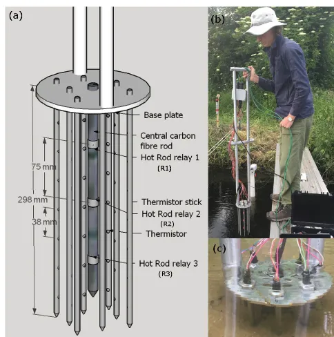
A 56-sensor, 3-D temperature array with three heat pulse sources (also known as the Hot Rod) was developed to mea-sure the flow direction and magnitude up to 200 mm be-low the water–sediment interface in the streambed (Fig. 1). The central carbon-fibre rod (260 mm long with a diame-ter of 12 mm) has three equally spaced, 60 W heating
ele-Figure 1. (a)Detailed design of the active HPS Hot Rod with three heating elements (R1, R2 and R3) on the central carbon-fibre rod surrounded by 56 temperature sensors at two distances from the central heat source (28 and 47 mm).(b)and(c)Installation of the Hot Rod in a small stream characterised by shallow bedforms.
ments along its length at positions of 65, 140 and 215 mm below the base plate and are referred to as heat injection depth R1, R2 and R3, respectively (Fig. 1). Eight stain-less steel rods (6 mm diameter and 298 mm long) housing seven equally spaced (38 mm apart) temperature thermistors (Maxim DS18B20; precision 0.06◦) are arranged cylindri-cally around the carbon-fibre rod and at two fixed spacings of 28 and 47 mm (Table S1 in the Supplement). The central rod and thermistor sticks are fixed to a rigid circular aluminium base plate which is attached to a collapsible handle. The ma-terial, dimensions and spacing of the rods to the base plate were designed to reduce flexibility and minimise disturbance to the sediment material on insertion, as this was a limitation in previous studies. A critical design feature was to ensure that the rods stayed parallel to one another and that the spac-ing did not vary durspac-ing installation, as it was designed to be used in a range of sedimentary environments from fine silt to coarse gravels.
[image:2.612.308.550.63.307.2]active heat pulse. The input current from the power supply regulator is also recorded each time the temperature is mea-sured to ensure a tight control on the actual power being de-livered through the heating elements to the surrounding ma-terial and therefore reducing uncertainty in the analysis rou-tine.
An important aspect of the design was that it could be rapidly and easily deployed to capture large spatial data sets along a reach of stream or across a pool–riffle sequence. In-stallation requires gently pushing (or lightly tapping with a shockless impact hammer) the device into the streambed ensuring that there is a sufficient gap between the top of the sediment and the underside of the base plate to prevent streamflow constriction (the top thermistor is set at 44 mm below the baseplate so a gap of∼30 mm puts the first ther-mistor just below the sediment–water interface). The impact of the installed device on flow velocity and direction is ex-pected to be minimal given that the volume of the device relative to the volume of the measurement area is less than 4 %.
Once installed and equilibrated with the surrounding sed-iment, the logger program is executed and the ambient tem-perature is measured at each thermistor (T0), directly fol-lowed by activation of the selected heat element for the cho-sen duration. The data logger records the temperature dif-ferential (1T =Tt−T0) at the chosen sample frequency to clearly discern the timing and location of the breakthrough curve at each of the thermistors. Field and laboratory tests showed that short, 1 min heat pulse injections and a 20– 30 min temperature response monitoring period are appropri-ate for estimating the dominant direction and flux magnitude in sandy streambeds. Specific details of the analysis routine that was used are described in the following section. 2.2 Data analysis and routine outputs
2.2.1 Heat transport simulation
The magnitude and direction of the water velocity at the ob-servation point based on the measured temperature break-through curves at the 56 sensors were determined using a modified version of the heat transport equation:
∂T
∂t = ∇ D
t∇T− ∇ ρ
wcw
ρc qT
, (1)
whereT is temperature (◦C) andDtis the thermal dispersion coefficient given as (de Marsily, 1986)
Dnt = κ0
ρc+βn·
ρwcw
ρc q , (2)
where κ0 is the bulk thermal conductivity of the water-saturated sediments (W m−1◦C−1), ρc is the volumetric heat capacity of the water-saturated sediments (J m−3◦C−1),
βn is the thermal dispersivity where the subscript n is
T for the transverse direction and L for the longitudinal direction, ρwcw is the volumetric heat capacity of water (4.1 J m−3◦C−1) andq is the Darcy velocity (or Darcy flux) of water (m s−1). WhereDLt ≈DTt, Eq. (2) can be simplified toDnt = κ0
ρc.
An analogy can be made to the solute transport equation where the mean water velocity is replaced with ρwcwρc q and the dispersion tensor can be replaced withDt. Assuming that these components are constant in space and time, Eq. (1) can be reduced to
∂T ∂t =D
t∇2T−ρwcw
ρc q∇T . (3)
An instantaneous injection of a thermal mass into an infi-nite three-dimensional sediment volume where there is only an x component of velocities can be defined as follows (Domenico and Schwartz, 1998):
T (x, y, z, t )= M0 8ρcDtL
1 2Dt
T(π t ) 3 2 exp −
x−ρwcw ρc qt
2
4DtLt −
y2+z2
4DtTt
, (4)
whereM0is the thermal mass (J).
The thermal mass input was not considered in previous studies as a known parameter (Angermann et al., 2012b). The Hot Rod, however, uses a known wattage, and the thermal mass term is given as
M0=F·dt, (5)
whereF is the heat flux and dtis the duration of application. The thermal mass input,M0, is measured by the data logger such that at full power the theoretical output of the 60 W heat-ing element provides 5 A of current and an injection period of 60 s equals an energy input of 3600 J.
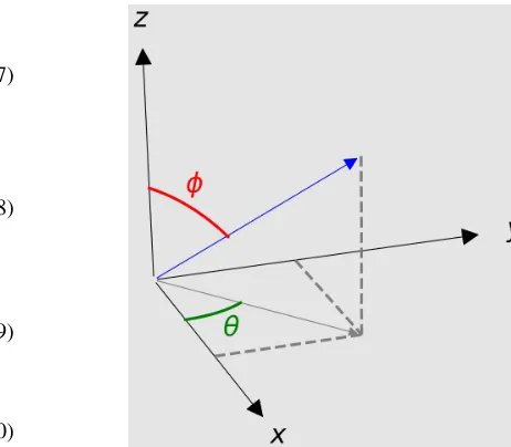
The requirement of Eq. (4) is that the flow component is only in thex direction, removing the non-diagonal compo-nents of the dispersion tensor. The aim of this paper is to define a flow direction and magnitude using a fixed sensor array, allowing the use of multiple sensors to constrain the thermal transport and flow properties. It is not always the case that the fluxes are oriented with the sensor array and therefore the location of the observations can be converted through rotation of the coordinate system, aligning the mea-surements relative to the flow direction. In this application we assume that the vector of Darcy fluxes in thex,y andz
direction is defined as
q= qx qy qz
. (6)
(Fig. 2), where
θ=tan−1
q
y
qx
. (7)
The rotational Jacobian matrix is then defined as
J=
cosθ sinθ 0 −sinθ cosθ 0
0 0 1
, (8)
the coordinates as
x0=Jx, (9)
and the flux as
q0=Jq. (10)
Secondly, we rotate the points around they axis. To do this we define the angleφ, where
φ=tan−1
q0 z q0 x . (11)
The rotational Jacobian matrix is then defined as
J=
cosφ 0 sinφ
0 1 0
−sinφ 0 cosφ
, (12)
the coordinates as
x00=Jx0, (13) and the flux as
q00=Jq0. (14) The transformation results in the representation of the Darcy fluxes as qx00= kqk (the magnitude of the non-transformed flow vector) andqy00=qz00=0. The distances of the sensors are oriented relative to this new flow vector. The main advan-tage over previous approaches is that all sensors can be in-cluded rather than a single sensor from the array accounting for a single transverse distance (Lewandowski et al., 2011).
We then substitute these new dimensions into Eq. (4) to get
T (x00, y00, z00, t )= M0 8ρcDtL12Dt
T(π t ) 3 2 ×exp −
x00−ρwcw ρc kqkt
2
4DLtt −
y002+z002
4DtTt
. (15)
[image:4.612.285.516.65.267.2]Equation (15) represents an impulse response function. The tests implemented used a finite pulse that did not meet this
Figure 2.Schematic showing the rotation of the coordinate system to determine anglesθandφ.
condition. As we assume that the properties are not temper-ature dependent, we can treat the contribution of multiple impulse responses as additive. Hence, Eq. (15) was imple-mented for a series of discrete, lagged pulses to represent the actual addition of thermal mass to the system. The use of discrete pulses is implemented as
Ttot(x00, y00, z00, t )= toff
X
τ=ton
T (x00, y00, z00, t−τ ), (16)
whereTtot is the total temperature response,ton is the time at which the heating element was turned on andtoff is the time when the heating element was turned off. The operatorτ
represents the time lags, and for each discrete pulseMo=F· dτ. The summedT term on the right-hand side is evaluated using Eq. (15) fort≥τ and is zero otherwise. This method allows for the representation of a non-Dirac heat pulse and also for variations in the input flux from the heating elements. The interval dτ was 3 s; hence, the Dirac representation was valid on a small scale.
2.2.2 Parameter estimation
Parameter estimation and uncertainty analysis was under-taken using the DREAM algorithm (Vrugt et al., 2009a, b). The fit of the data was performed by assessing the likelihood of each individual model run. The likelihood is defined as
L= − nobs X
1 lnpobs
Tmod|Tobs, σ2
+ npars X
1
ln ppar(X)
!
, (17)
distri-Table 1.Initial parameter values forkqk,θ,φ,κ0andρcused in
the analysis routine. A uniform distribution of the five parameters was used.
Parameter Mean Width
kqk– magnitude (m s−1) 10−5 103
κ0(W m−1◦C−1) 3 1.25
ρc(J m−3◦C−1) 2 750 000 1 500 000
θ π 2π
φ π 2π
bution and a mean ofTobsand a variance ofσ2; andppar rep-resents the probability of the parameter X. We assume that the parameters are uniformly distributed; hence,ppar(X)=1 when the parameters are in bounds and zero elsewhere.
The DREAM method is an adaption of the standard Markov chain Monte Carlo method. The technique is ini-tialised by specifying a number of chains. Each chain re-ceives starting parameters by randomly sampling the param-eter ranges (Table 1). After calculating an initial likelihood for the starting parameters, the algorithm selects proposed parameter values using the other chains, and the likelihood of these model parameters are also calculated. If the likelihood of these parameters is greater than the current parameters, the new parameters are accepted; however, if the likelihood of the new parameters is lower, the transition probability is calculated using a ratio of the likelihoods, and the transition is determined by generating a random number. The method is explained in greater detail in Vrugt et al. (2009c). The gen-eral outcome is that the chains spend a greater amount of time in locations of more favourable parameters, and the distribu-tion of these parameters represents the posterior distribudistribu-tion of the parameter probabilities, given the model, the data and the prior knowledge of the parameter distributions.
The optimisation was undertaken using five parameters: kqk, θ, φ, κ0 and ρc. All of the parameters in the ther-mal dispersion term (Eq. 2) cannot be identified simultane-ously in the optimisation, resulting in non-convergence of the Markov Chain approach because of the correlation between the thermal dispersivity flow term and the thermal conduc-tivity. In the experiments that we conducted we found that the longitudinal and transverse dispersion terms, DLt ≈DtT
and therefore Eq. (2) can be simplified to Dnt =κ0
ρc. Hence, κ0was included as an optimisation parameter and it was also physically measured in the experiments. The default param-eter likelihoods and initial distributions were taken from the ranges presented in Table 1. The error of the temperature ob-servations (σ) was taken to be 0.06◦C, the precision of the temperature sensors. Whilst the model parameters are esti-mated using angle and the flow magnitude, the actual flow vector can be recovered as
q=
"kqkcos(φ)cos(θ )
kqkcos(φ)sin(θ )
kqksin(φ)
#
. (18)
2.3 Laboratory sand tank
A laboratory sand tank was used to provide a controlled en-vironment on the hydraulic regime to test the performance of the Hot Rod and so that the different flux calculation meth-ods could be compared. A total of 36 combinations of flow direction, magnitude and depth of heat pulse were used. The dimensions of the sand tank for each of the scenarios varied slightly according to the fixed boundary conditions (Fig. 3). Four flow scenarios were tested: (1) horizontal flow from left to right (inflow and outflow occurred over the entire satu-rated cross-sectional area of the sediment volume on the left and right boundaries of the tank), (2) diagonal flow from the top left to bottom right (inflow was through a 20 mm hori-zontal inlet slit on the top left boundary and outflow through a 20 mm horizontal slit, 85 mm above the base of the right boundary), (3) upward flow (inflow occurred over the cross-sectional area of the base of the tank and outflow at the top of the sediment at overflow points above the sediment on the left and right boundaries), and (4) downward flow (in-flow was distributed over the cross-sectional area of the sed-iment surface and outflow via the cross-sectional area of the tank base). A steady state flow regime for each scenario was maintained by constant heads at the inflow and outflow ports of the tank and the use of a peristaltic pump with a highly accurate ultrasonic flowmeter (Atrato ultrasonic flowmeter; 0.05 % linearity on flow less than 5 L min−1) to ensure a con-stant discharge rate. The flowmeter data were also used to determine the Darcy flux for the different flow conditions. Fine perforated mesh was used to contain the sediment and to provide the necessary flow conditions along each of the tank boundaries. The hydraulic conductivity and thermal hy-draulic conductivity of the graded, saturated sand were mea-sured using a KSAT meter (UMS GmbH, Munich, Germany) and KD2 Pro (Decagon, Washington, USA), respectively. Three different hydraulic gradients and discharge rates for the four flow scenarios were conducted to capture low- (∼ 10−6m s−1), moderate- (∼10−5m s−1) and high-flow con-ditions (∼10−4m s−1). The Hot Rod was positioned in the middle of the sand tank with thermistor stick sensor number one orientated perpendicular (90◦) to the flow direction for all of the scenarios. To validate the spatial arrangement of the sensors, the horizontal flow scenario was repeated with ther-mistor stick sensor number one rotated to be 45◦ to the di-rection of flow. In addition to these flow scenarios, a no-flow experiment was conducted to evaluate the analysis routine, where the boundary conditions meant that there was stagnant water.
2.4 Experimental field site
Figure 3.Laboratory sand tank dimensions for each of the flow scenarios:(a)horizontal flow,(b)diagonal flow,(c)upward flow and(d) downward flow.
treatment facility. The geomorphology of the river was char-acterised by a narrow channel, no more than 3 m wide with 0.3–0.5 m deep sediment ranging from fine silt to coarse gravels overlying a tight, low-permeability clay. The selec-tion of this field site was part of another ongoing investi-gation looking at attenuation of micro-pollutants in the hy-porheic zone. The residence time in the hyhy-porheic zone was critical in evaluating the stream attenuation modelling.
3 Results and discussion 3.1 Laboratory sand tank
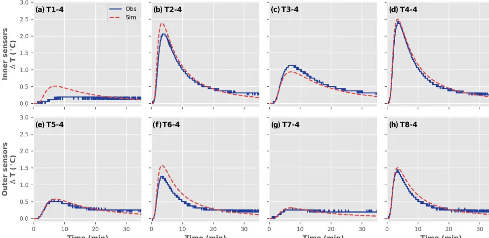
Overall, the modelled breakthrough curves closely fit the observed data from the 56-sensor array with the modelled curves capturing the rising limb, peak and tail of the mea-sured temperature data over the sample period (Fig. 3). The variance of each parameter is included in the mod-elled temperature breakthrough curves; however, the
Figure 4.Breakthrough curves shown of the fourth vertical thermistor (158 mm depth) from each radial sensor location for the horizontal flow scenario from heat injection depth at relay 2. Solid lines are observed and dashed lines are modelled.
curves from the diagonal flow scenario showed a similar re-sponse in those sensors up- and down-gradient of the heat pulse (Fig. S1a). In the upward and downward flow sce-narios there was very little response in the outer thermis-tor sensors due to the dominant vertical component of flow (Fig. S1b–c). This low response of the outer sensors was even more pronounced under higher flow conditions in the upward and downward flow scenarios. The 3-D time series videos showed clearly the migration of the heated plume vertically and highlighted the complexity of fitting multiple breakthrough curves to the most likely solution (refer to the video file in https://doi.org/10.4226/86/5aab1b67337bb).
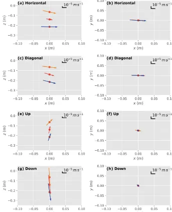
Overall, the 3-D flow fields calculated from the HPS Hot Rod in the laboratory sand tank for the four flux scenarios and heat injection depths (65, 140 and 215 mm) were consis-tent with the flow conditions established in the tank (Fig. 5). Under left to right horizontal flow conditions (Fig. 5a and b), the modelled direction of flow from each of the heat injection depths is very similar with some slight offset to the observed flow in theydirection, which was perpendicular to thermis-tor stick sensor 1 (90◦to the flow direction). There was also a slight deviation downwards in thezdirection, particularly for the shallowest heat injection depth. To refute any bias in the optimisation routine and the array configuration, the Hot Rod was rotated by 45◦for the horizontal flow scenario and
it showed a very similar output to when it was orientated 90◦ to the flow direction.
Results from the other three scenarios showed that the modelled flux direction is close to parallel to the flow
con-ditions established in the tank and the magnitude of the flux was similar at each of the heat injection depths (Fig. 5c–h). Reviewing the time series data in the 3-D plots (Supplement), the spreading of the heat pulse from the heat injection depth can be clearly detected, indicating how the heat pulse moves along the established flow line. The thermistor highlighted in blue in the 3-D plot was the sensor that showed the maximum temperature breakthrough curve and clearly shows a different orientation to the most likely flux direction (black arrow) as determined by the DREAM algorithm.
Some discrepancies in the direction of the modelled flow and differences in flux magnitude at each heat injection depth may be attributed to (1) placement orientation and the angle of the sensor positions of the Hot Rod relative to the flow conditions established in the tank, (2) boundary conditions in the tank to establish flow and (3) the fact that the optimi-sation routine determines the best fit of all the observed data in a 3-D volume around the heat injection depth rather than at a specific point.
Figure 5.Calculated fluxes and directions for the four flow scenarios at each of the heat injection depths:(a, b)horizontal,(c, d)diagonal, (e, f)upward and(g, h)downward flow scenarios.
the optimisation routines for particular flow conditions i.e. strongly upwards flow.
In the case of no-flow conditions established in the sand tank (Fig. S2), the optimisation routine fitted the measured temperature breakthrough data; however, on closer inspec-tion of the 3-D time series plot it was evident based on the uniform heat plume around the heat injection point during the injection period that heat transport was by conduction only. Absence of clear advective movement of the heat pulse and a calculated flux less than about∼10−6m s−1indicated the lower limit of the active heat pulse sensor.
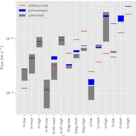
The flux magnitude (kqk) of the different flow scenarios and different flow intensities calculated based on different heat injection depths of the HPS (grey bars) compared to the
fluxes determined based on Darcy’s law (hydraulic gradient and hydraulic conductivity) and the measured discharge from the tank using an ultrasonic flowmeter is shown in Fig. 6 and Table S2.
Figure 6. Fluxes of the different flow scenarios, listed along the
x axis, and different flow intensities calculated based on different heat injection depths of the HPS (grey bars) compared to fluxes de-termined based on Darcy’s law (hydraulic gradient and hydraulic conductivity – red dashes) and the flux calculated from the mea-sured discharge from the tank using an ultrasonic flowmeter and the cross-sectional area of the tank (blue dashes).
conductivity increases with decreasing porosity (Smits et al., 2010).
Histograms of the flux magnitude (kqk) and flux compo-nents in thex,y andzdirection for the combination of most likely parameter values used in the DREAM algorithm were generated for each measurement. The results from heat in-jection depth R2 for the horizontal flow scenario is shown in Fig. S3, which shows that the distribution is tightly con-strained. This is also evident in cross correlation plots of the flux magnitude, thermal conductivity and the specific heat capacity (Fig. S4).
Constraining the range of the thermal conductivity val-ues used in the optimisation routine to the known measured thermal conductivity of the sand from the KD2 Pro instru-ment showed little impact on the calculated flux magnitude. However, comparing the modelled breakthrough curves from two optimisations when the range in thermal conductivity was limited to the measured known thermal conductivity (3 W m−1◦C−1) in one model and in the other model it used a value of 3.52 W m−1◦C−1(for a best fit from a range of val-ues from 2.5 to 4.5 W m−1◦C−1) showed there were subtle differences between the modelled breakthrough curve peak and falling limbs (Fig. 7).
Our study found that the inclusion of longitudinal and transverse thermal dispersion had less than a 2 % difference on the mean calculated fluxes. The study by Rau et al. (2012)
determined Darcy velocities derived from heat experimenta-tion that included the thermal dispersivity term differed by up to 20 % when compared to solute experimentation. However, other studies in the literature have shown that there is con-siderable uncertainty on the magnitude of the thermal disper-sivity (Anderson, 2005). Thermal disperdisper-sivity has also been found not to be scale-dependent such as solute dispersivity because heat transport happens through the pore water and through the sediment matrix (Vandenbohede et al., 2009). Therefore, given the scale that we are working at (few cen-timetres) and also the low velocities, the effect on the calcu-lated flux is likely to be negligible.
3.2 Experimental field site
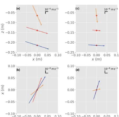
The measured 3-D flow fields at the experimental site showed considerable variability in the direction of flow and flux mag-nitude over∼0.20 m depth of the streambed. The flux mag-nitude at the six stations along the river at the three heat injection depths (0.065, 0.140 and 0.215 m) ranged from 4.2×10⁻⁶to 4.26×10⁻⁵m s−1(mean: 1.6×10⁻⁵m s−1). At each of the stations, the component of horizontal flow com-pared to vertical flow within the streambed was dominant. It was only at the shallowest heat injection depth, just below the stream bed surface, that there was a greater component of vertical flow. The results from two of the six stations are shown in Fig. 8, where the Hot Rod was positioned in the streambed such that thex axis of the figure was aligned to the direction of stream flow. In such environments the flow direction is driven by the surface flow and the geomorpho-logical features of the streambed. Small bed structures such as ripples will only impact the hyporheic flow field in the uppermost centimetres of the sediment, which is a plausible explanation as to what was observed from the outputs of the Hot Rod.
Figure 7.Comparison of the observed (blue line) and modelled breakthrough curves for selected temperature sensors (T x−x) when the thermal conductivity,κ0, of the sediment has a known value of 3 W m−1◦C−1(orange graph) and when the model is provided with a range of plausible values from 2.5 to 4.5 W m−1◦C−1resulting in 3.52 W m−1◦C−1(red graph).
Figure 8.Calculated fluxes and flux directions at the three heat in-jection depths from two of the stations at the experimental field site. (a, b) Station 1 and(c, d)Station 2. Thexaxis in the figures is positive in the direction of streamflow.
in particular differences in the horizontal and vertical flux components. Additional measurements of the streambed sed-iments would provide a tighter constraint on the parameter set used in the optimisation; however, the parameter estima-tion and uncertainty analysis routine does successfully fit the measured data to provide a reliable estimate of the flux and its direction. Refer to Banks et al. (2017) for all of the tem-perature data files from the sand tank and experimental site, available at https://doi.org/10.4226/86/5aab1b67337bb.
4 Conclusions
[image:10.612.64.270.449.653.2]cur-rent input; and (4) lack of a suitable optimisation routine to determine the most likely set of parameters to constrain the data and an uncertainty analysis on the flux magnitude and its direction.
The rigidity and robustness of the Hot Rod and use of heating elements at three different vertical positions provided a method to examine how the flux and its direction varied vertically with depth beneath the streambed interface at indi-vidual locations in a range of different environmental settings and sediment types. The use of two horizontal spacings be-tween the heating elements and thermistors as well as addi-tional thermistors at multiple angles to the heating elements increased confidence in the measurement of heat transport processes and tightened the optimisation routine of the tem-perature data. The addition of the measured input of energy at the heating element in the heat transport equation as a se-ries of discrete heat pulses over the injection period provided one less unknown variable to calibrate against. In many of the experiments conducted in the sand tank and at the ex-perimental site, the optimisation routine using the DREAM algorithm showed that the most likely flux direction from the heat injection depth was not towards the sensor that showed the maximum temperature breakthrough because it uses all of the sensor temperature breakthrough curves in the analysis. The 3-D time series plot was a valuable tool in assessing this result and it also showed whether heat transport was domi-nated by diffusion and/or conduction with radial symmetry around the heating element or whether there was convective heat flow. This interrogation process was found to be critical in the data assessment to ensure that the model did not over-fit the measured data with unrealistic physical values for the sediment and heat transport conditions.
The laboratory and experimental field site applications us-ing the DREAM algorithm for parameter estimation and un-certainty analysis demonstrated the performance of the ac-tive heat-pulse-sensing instrument (the Hot Rod) to measure the multi-directional 3-D-flow fields and fluxes in the near-surface streambed. Active heat pulse sensing provides a num-ber of advantages over other approaches that have investi-gated hyporheic exchange, including the low cost of data collection and the rapid assessment of small physical pro-cesses that can be undertaken on a reach scale. Marzadri et al. (2013) showed that the hyporheic residence time, which is influenced by the streambed physical morphology and in-stream flow discharge, ultimately determines the spatially complex patterns of the time-varying thermal regime within the hyporheic zone. The short-duration active heat pulse sensing helped overcome some of the challenges in mea-suring the water temperatures because of the stronger signal from the heat pulse.
Most other studies that use heat as a tracer assume 1-D flow only and the lateral or horizontal component is not con-sidered. Studies that have identified the geometry of the sub-surface flow field using a polynomial model fitted to the am-plitude ratio of the vertical temperature profiles were only
able to determine the deviation from one-dimensional verti-cal flow (Munz et al., 2016). Errors in the vertiverti-cal component of flow have been shown to progressively increase with the magnitude of the horizontal flow component (Lautz, 2010). The 3-D analysis routine and sensor arrangement applied in this study were able to capture all three components of the flow field around the point of observation. The importance of capturing the multi-directional flow field was clearly demon-strated in the sand tank under an extensive range of flow con-ditions that would be anticipated in a dynamic stream envi-ronment. Measurements of the hydraulic gradient and char-acterising the physical properties of the streambed sediment are also important in understanding the dynamic exchange processes within the hyporheic zone and the very transient nature of such environments.
The concept and design of the active heat-pulse-sensing instrument could also be adapted to other hydrological re-search areas, including the measurement of shallow interflow along hillslopes and discharge from groundwater seeps and springs.
Data availability. Data are available at https://doi.org/10.4226/ 86/5aab1b67337bb (Banks, 2017).
Supplement. The supplement related to this article is available online at: https://doi.org/10.5194/hess-22-1917-2018-supplement.
Competing interests. The authors declare that they have no conflict of interest.
Acknowledgement. We are grateful to Flinders University South Australia for a small grant to develop the HPS Hot Rod and all Faculty of Science and Engineering technical workshop staff for their assistance in hardware development and construction. Funding support from the Australian Research Council (ARC) Linkage Project LP150100588 is acknowledged. Additional fund-ing through the Australia–Germany Joint Research Cooperation Scheme of Universities Australia and the German Academic Exchange Service (DAAD, grant no. 57216806) provided support for fieldwork collaboration between the research institutes.
Edited by: Thom Bogaard
Reviewed by: Jim Constantz and Bas des Tombe
References
Abu-Hamdeh, N. H.: Thermal properties of soils as affected by density and water content, Biosyst. Eng., 86, 97–102, https://doi.org/10.1016/S1537-5110(03)00112-0, 2003. Anderson, M. P.: Heat as a ground water tracer, Ground Water, 43,
Angermann, L., Krause, S., and Lewandowski, J.: Application of heat pulse injections for investigating shallow hyporheic flow in a lowland river, Water Resour. Res., 48, W00P02, https://doi.org/10.1029/2012WR012564, 2012a.
Angermann, L., Lewandowski, J., Fleckenstein, J. H., and Nütz-mann, G.: A 3D analysis algorithm to improve interpretation of heat pulse sensor results for the determination of small-scale flow directions and velocities in the hyporheic zone, J. Hydrol., 475, 1–11, https://doi.org/10.1016/j.jhydrol.2012.06.050, 2012b. Bakker, M., Caljé, R., Schaars, F., van der Made, K.-J., and
de Haas, S.: An active heat tracer experiment to determine groundwater velocities using fiber optic cables installed with direct push equipment, Water Resour. Res., 51, 2760–2772, https://doi.org/10.1002/2014WR016632, 2015.
Ballard, S.: The in situ permeable flow sensor: a ground-water flow velocity meter, Ground Water, 34, 231–240, https://doi.org/10.1111/j.1745-6584.1996.tb01883.x, 1996. Banks, E. W., Shanafield, M. A., and Cook, P. G.:
In-duced temperature gradients to examine groundwater flowpaths in open boreholes, Groundwater, 52, 943–951, https://doi.org/10.1111/gwat.12157, 2014.
Banks, E.: Temperature time series data for active HPS Hot Rod, Flinders University, https://doi.org/10.4226/86/5aab1b67337bb, 2017.
Barry-Macaulay, D., Bouazza, A., Singh, R. M., Wang, B., and Ranjith, P. G.: Thermal conductivity of soils and rocks from the Melbourne (Australia) region, Eng. Geol., 164, 131–138, https://doi.org/10.1016/j.enggeo.2013.06.014, 2013.
Boulton, A. J., Findlay, S., Marmonier, P., Stanley, E. H., and Valett, H. M.: The functional significance of the hyporheic zone in streams and rivers, Annu. Rev. Ecol. Syst., 29, 59–81, 1998. Briggs, M. A., Lautz, L. K., McKenzie, J. M., Gordon, R. P.,
and Hare, D. K.: Using high-resolution distributed tempera-ture sensing to quantify spatial and temporal variability in vertical hyporheic flux, Water Resour. Res., 48, W02527, https://doi.org/10.1029/2011WR011227, 2012.
Brunke, M. and Gonser, T.: The ecological significance of exchange processes between rivers and groundwater, Freshwater Biol., 37, 1–33, 1997.
Caissie, D.: The thermal regime of rivers: a review, Fresh-water Biol., 51, 1389–1406, https://doi.org/10.1111/j.1365-2427.2006.01597.x, 2006.
Constantz, J., Stewart, A. E., Niswonger, R., and Sarma, L.: Analysis of temperature profiles for investigating stream losses beneath ephemeral channels, Water Resour. Res., 38, 1–13, https://doi.org/10.1029/2001WR001221, 2002.
Constantz, J., Eddy-Miller, C. A., Wheeler, J. D., and Es-said, H. I.: Streambed exchanges along tributary streams in humid watersheds, Water Resour. Res., 49, 2197–2204, https://doi.org/10.1002/wrcr.20194, 2013.
Constantz, J., Naranjo, R., Niswonger, R., Allander, K., Neilson, B., Rosenberry, D., Smith, D., Rosecrans, C., and Stonestrom, D.: Groundwater exchanges near a channelized versus unmodified stream mouth discharging to a subalpine lake, Water Resour. Res., 52, 2157–2177, https://doi.org/10.1002/2015WR017013, 2016.
de Marsily, G.: Quantitative Hydrogeology: Groundwater Hydrol-ogy for Engineers, Academic Press, Cambridge, Massachusetts, United States, 1986.
Domenico, P. A. and Schwartz, F. W.: Physical and Chemical Hy-drogeology, vol. 1, Wiley, New Jersey, United States, 1998. Engelhardt, I., Prommer, H., Moore, C., Schulz, M., Schüth, C.,
and Ternes, T. A.: Suitability of temperature, hydraulic heads, and acesulfame to quantify wastewater-related fluxes in the hy-porheic and riparian zone, Water Resour. Res., 49, 426–440, https://doi.org/10.1029/2012WR012604, 2013.
Gandy, C. J., Smith, J. W. N., and Jarvis, A. P.: Attenuation of mining-derived pollutants in the hyporheic zone: a review, Sci. Total Environ., 373, 435–446, 2007.
Gomez-Velez, J. D., Harvey, J. W., Cardenas, M. B., and Kiel, B.: Denitrification in the Mississippi River network controlled by flow through river bedforms, Nat. Geosci., 8, 941–945, https://doi.org/10.1038/ngeo2567, 2015.
Greswell, R. B., Riley, M. S., Alves, P. F., and Tellam, J. H.: A heat perturbation flow meter for application in soft sediments, J. Hy-drol., 370, 73–82, https://doi.org/10.1016/j.jhydrol.2009.02.054, 2009.
Harvey, J. W., Böhlke, J. K., Voytek, M. A., Scott, D., and Tobias, C. R.: Hyporheic zone denitrification: con-trols on effective reaction depth and contribution to whole-stream mass balance, Water Resour. Res., 49, 6298–6316, https://doi.org/10.1002/wrcr.20492, 2013.
Harvey, W. H. and Wagner, B. J.: Quantifying hydrologic interac-tions between streams and their subsurface hyporheic zones, in: Streams and Ground Waters, edited by: Jones, J. B. and Mulhol-land, P. J., Academic Press, San Diego, 3–44, 2000.
Jury, W. A. and Horton, R.: Soil Physics, 6th Edn., John Wiley, New Jersey, United States, 2004.
Kurth, A.-M., Weber, C., and Schirmer, M.: How effective is river restoration in re-establishing groundwater–surface water interac-tions? – A case study, Hydrol. Earth Syst. Sci., 19, 2663–2672, https://doi.org/10.5194/hess-19-2663-2015, 2015.
Lautz, L. K.: Impacts of nonideal field conditions on vertical water velocity estimates from streambed temperature time series, Water Resour. Res., 46, 1–14, https://doi.org/10.1029/2009WR007917, 2010.
Lewandowski, J., Angermann, L., Nützmann, G., and Fleck-enstein, J. H.: A heat pulse technique for the determina-tion of small-scale flow direcdetermina-tions and flow velocities in the streambed of sand-bed streams, Hydrol. Process., 25, 3244– 3255, https://doi.org/10.1002/hyp.8062, 2011.
Marzadri, A., Tonina, D., and Bellin, A.: Effects of stream morpho-dynamics on hyporheic zone thermal regime, Water Resour. Res., 49, 2287–2302, https://doi.org/10.1002/wrcr.20199, 2013. Munz, M., Oswald, S. E., and Schmidt, C.: Analysis of riverbed
temperatures to determine the geometry of subsurface water flow around in-stream geomorphological structures, J. Hydrol., 539, 74–87, https://doi.org/10.1016/j.jhydrol.2016.05.012, 2016. Naranjo, R. C. and Turcotte, R.: A new temperature
pro-filing probe for investigating groundwater-surface wa-ter interaction, Water Resour. Res., 51, 7790–7797, https://doi.org/10.1002/2015WR017574, 2015.
Rau, G. C., Andersen, M. S., and Acworth, R. I.: Experimental in-vestigation of the thermal dispersivity term and its significance in the heat transport equation for flow in sediments, Water Resour. Res., 48, 1–21, https://doi.org/10.1029/2011WR011038, 2012. Rau, G. C., Andersen, M. S., McCallum, A. M., Roshan, H.,
and Acworth, R. I.: Heat as a tracer to quantify water flow in near-surface sediments, Earth-Sci. Rev., 129, 40–58, https://doi.org/10.1016/j.earscirev.2013.10.015, 2014.
Read, T., Bour, O., Selker, J. S., Bense, V. F., Le Borgne, T., Hochreutener, R., and Lavenant, N.: Active-distributed temperature sensing to continuously quantify vertical flow in boreholes, Water Resour. Res., 50, 3706–3713, https://doi.org/10.1002/2014wr015273, 2014.
Sellwood, S. M., Bahr, J. M., and Hart, D. J.: Evaluation of a discrete-depth heat dissipation test for thermal characteriza-tion of the subsurface, Geol. Soc. Am. Spec. Pap., 519, 67–79, https://doi.org/10.1130/2016.2519(05), 2016.
Shanafield, M., Pohll, G., and Susfalk, R.: Use of heat-based verti-cal fluxes to approximate total flux in simple channels, Water Re-sour. Res., 46, W03508, https://doi.org/10.1029/2009wr007956, 2010.
Shanafield, M., McCallum, J. L., Cook, P. G., and Noorduijn, S.: Variations on thermal transport modelling of subsurface temper-atures using high resolution data, Adv. Water Resour., 89, 1–9, https://doi.org/10.1016/j.advwatres.2015.12.018, 2016. Smits, K. M., Sakaki, T., Limsuwat, A., and Illangasekare, T. H.:
Thermal conductivity of sands under varying moisture and poros-ity in drainage–wetting cycles, Vadose Zone J., 9, 172–180, https://doi.org/10.2136/vzj2009.0095, 2010.
Su, G., Freifeld, B., Oldenburg, C., Jordan, P., and Da-ley, P.: Interpreting Velocities from Heat-Based Flow Sen-sors by Numerical Simulation, Ground Water, 44, 386–393, https://doi.org/10.1111/j.1745-6584.2005.00147.x, 2006.
Vandenbohede, A., Louwyck, A., and Lebbe, L.: Conser-vative solute versus heat transport porous media dur-ing push-pull tests, Transport Porous Med., 76, 265–287, https://doi.org/10.1007/s11242-008-9246-4, 2009.
Vogt, T., Schneider, P., Hahn-Woernle, L., and Cirpka, O. A.: Esti-mation of seepage rates in a losing stream by means of fiber-optic high-resolution vertical temperature profiling, J. Hydrol., 380, 154–164, https://doi.org/10.1016/j.jhydrol.2009.10.033, 2010. Vrugt, J. A., Robinson, B. A., and Hyman, J. M.:
Self-adaptive multimethod search for global optimization in real-parameter spaces, IEEE T. Evolut. Comput., 13, 243–259, https://doi.org/10.1109/TEVC.2008.924428, 2009a.
Vrugt, J. A., ter Braak, C. J. F., Diks, C. G. H., Robinson, B. A., Hy-man, J. M., and Higdon, D.: Accelerating Markov Chain Monte Carlo Simulation by differential evolution with self-adaptive ran-domized subspace sampling, Int. J. Nonlinear Sci., 3, 273–290, 2009b.
Vrugt, J. A., ter Braak, C. J. F., Gupta, H. V., and Robinson, B. A.: Equifinality of formal (DREAM) and informal (GLUE) Bayesian approaches in hydrologic modeling?, Stoch. Env. Res. Risk A., 23, 1011–1026, https://doi.org/10.1007/s00477-008-0274-y, 2009c.