www.hydrol-earth-syst-sci.net/17/4043/2013/ doi:10.5194/hess-17-4043-2013
© Author(s) 2013. CC Attribution 3.0 License.
Hydrology and
Earth System
Sciences
Sequential and joint hydrogeophysical inversion using a field-scale
groundwater model with ERT and TDEM data
D. Herckenrath1,2, G. Fiandaca3,4, E. Auken3, and P. Bauer-Gottwein1
1Technical University of Denmark, Dept. of Environmental Engineering, Miljøvej, Building 113, 2800,
Kgs. Lyngby, Denmark
2Flinders University, National Centre for Groundwater Research and Training, G.P.O. Box 2100, Adelaide,
SA 5001, Australia
3Aarhus University, Dept. of Earth Sciences, Høegh-Guldbergs Gade 2, 8000, Aarhus C, Denmark 4University of Palermo, Dept. of Mathematics and Computer Science, Palermo, Italy
Correspondence to: D. Herckenrath ([email protected])
Received: 1 February 2013 – Published in Hydrol. Earth Syst. Sci. Discuss.: 11 April 2013 Revised: 28 August 2013 – Accepted: 11 September 2013 – Published: 18 October 2013
Abstract. Increasingly, ground-based and airborne geophys-ical data sets are used to inform groundwater models. Re-cent research focuses on establishing coupling relationships between geophysical and groundwater parameters. To fully exploit such information, this paper presents and compares different hydrogeophysical inversion approaches to inform a field-scale groundwater model with time domain electromag-netic (TDEM) and electrical resistivity tomography (ERT) data. In a sequential hydrogeophysical inversion (SHI) a groundwater model is calibrated with geophysical data by coupling groundwater model parameters with the inverted geophysical models. We subsequently compare the SHI with a joint hydrogeophysical inversion (JHI). In the JHI, a geo-physical model is simultaneously inverted with a groundwa-ter model by coupling the groundwagroundwa-ter and geophysical pa-rameters to explicitly account for an established petrophysi-cal relationship and its accuracy. Simulations for a synthetic groundwater model and TDEM data showed improved esti-mates for groundwater model parameters that were coupled to relatively well-resolved geophysical parameters when em-ploying a high-quality petrophysical relationship. Compared to a SHI these improvements were insignificant and geophys-ical parameter estimates became slightly worse. When em-ploying a low-quality petrophysical relationship, groundwa-ter model paramegroundwa-ters improved less for both the SHI and JHI, where the SHI performed relatively better. When comparing a SHI and JHI for a real-world groundwater model and ERT data, differences in parameter estimates were small. For both
cases investigated in this paper, the SHI seems favorable, tak-ing into account parameter error, data fit and the complexity of implementing a JHI in combination with its larger compu-tational burden.
1 Introduction
1 2
Fig. 1 SHI (left), CHI (middle) and JHI approach (right). π and γ respectively indicate the geophysical and groundwater model parameters, where the 3
arrows represent parameter updating until a minimum data and/or constraint misfit is achieved. π: geophysical model parameters; γ: groundwater model 4
parameters. 5
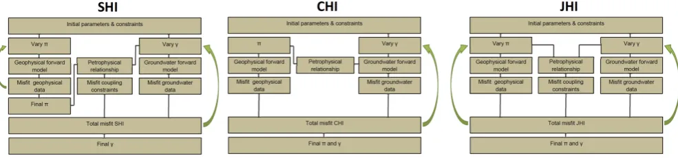
Fig. 1. SHI (left), CHI (middle) and JHI approach (right).πandγrespectively indicate the geophysical and groundwater model parameters, where the arrows represent parameter updating until a minimum data and/or constraint misfit is achieved.π: geophysical model parameters;
γ: groundwater model parameters.
A major challenge is to fully exploit the information con-tent of geophysical data sets, as geophysical techniques do not measure hydrological subsurface properties directly. A geophysical inversion and petrophysical relationships are needed to estimate hydrogeological parameters and state variables from the geophysical data sets. For this reason, the inclusion of geophysical data into a groundwater model is not straightforward. Previous studies have used different approaches to inform groundwater models with geophysical data.
1.1 Hydrogeophysical inversion approaches
Hydrogeophysical inversion approaches can be subdivided into sequential hydrogeophysical inversion (SHI), coupled hydrogeophysical inversion (CHI) and joint hydrogeophys-ical inversion (JHI) (Hinnell et al., 2010). The workflow as-sociated with these 3 methods is shown in Fig. 1.
1. In a SHI, geophysical data is separately inverted to es-timate the distribution of a geophysical property (e.g., maps of electrical resistivity). Estimated geophysical property maps are subsequently used to derive the structure of the subsurface or to estimate dynamic state variables such as solute concentrations and wa-ter content. For the latwa-ter, petrophysical relationships (Archie, 1942; Topp et al., 1980) are needed to convert a geophysical property to a hydrological state variable. Note Fig. 1 only shows an SHI in which inverted geo-physical parameters are coupled with the static input structure of a hydrological model; SHI by coupling dynamic state variables would typically require cou-pling inverted geophysical parameters with hydrologic model output.
2. In a CHI, simulated state variables of a hydrologi-cal model are transformed to a geophysihydrologi-cal parameter distribution using a petrophysical relationship. Subse-quently, geophysical forward responses are simulated that can be compared with collected geophysical ob-servations. In this approach, the geophysical inversion
process is coupled with the hydrological model and a single objective function is minimized that comprises both a geophysical and a hydrological component. 3. In a JHI, a simultaneous inversion for multiple
geo-physical and/or hydrological models is undertaken to exploit differences in parameter resolution for differ-ent data sets. In the JHI discussed in this paper, input parameters of a hydrological and geophysical model are simultaneously estimated using parameter cou-pling constraints to account for observed correlations between geophysical and groundwater model parame-ters (e.g., petrophysical relationships).
[image:2.595.53.546.64.179.2]structures and parameter distributions with geophysical and hydrological data (Hyndman and Gorelick, 1996; Chen et al., 2006; Linde et al., 2006b; Herckenrath et al., 2012a).
In comparison with a SHI, the main strength of a CHI is to use a hydrological model to provide an inversion framework for the geophysical data and constrain the geophysical inver-sion process. This brings two main advantages, as (1) mea-surement errors and parameter uncertainties associated with the independent geophysical inversion are not propagated di-rectly to the hydrological model and (2) no extensive regu-larization (e.g., smoothness constraints) is needed to stabilize the geophysical inversion process (Menke, 1984). These reg-ularization constraints do not necessarily reflect the hydro-logical conditions (Day-Lewis et al., 2005; Chen et al., 2006; Slater, 2007) and in a CHI these are substituted by spatial correlation structures provided by a hydrological model. In simple words, the hydrological model provides an interpre-tation framework for the geophysical data.
The advantage of joint inversion/JHI with respect to SHI is the exploitation of parameter resolution differences for dif-ferent data types (Linde et al., 2006a). Concerns pertaining to joint inversion for multiple geophysical methods are mainly related to observation weighting strategies and the transfer of correlated measurement error. When different model types and setups are used, as in a JHI, transfer of conceptual model errors is an additional problem.
In this study we confront the SHI and JHI approaches, without focusing on the JHI and CHI comparison, as these latter methods cannot easily act as substitute for one another. This is due to the different nature of coupling between the hydrologic and geophysical model. In a CHI, hydrological simulations are coupled with geophysical models while JHI couples input parameters.
However, JHI and CHI share similar concerns regarding the propagation of hydrological conceptual model errors, the definition of petrophysical relationships and the assignment of weights for various data types. The propagation of hydro-logical conceptual errors to the geophysical model differs for SHI, CHI and JHI. In a SHI no conceptual hydrological er-rors propagates into the geophysical model, but this will be the case in CHI and JHI. The difference between the latter two methods is that CHI generally employs a single concep-tualization for both the geophysical and hydrological model while JHI allows different conceptualizations for the geo-physical and hydrological model. Further discussion of this topic is beyond the scope of this paper, as this problem will be highly dependent on considered models, available data sets, the purpose of the hydrogeophysical inversion process and the employed petrophysical relationships.
1.2 Petrophysical and geometric relationships
Any hydrogeophysical modeling approach (SHI, CHI or JHI) depends on coupling geophysical and hydrological models by implementing coupling relationships between
geophysical parameters with hydrological model parame-ters or hydrological model simulations. Such coupling re-lationships can be sub-divided in different groups. In this paper, we consider petrophysical and geometric relation-ships. Well-known petrophysical relationships are Archie’s law (Archie, 1942) and the Topp equation (Topp et al., 1980), that respectively link electrical resistivity and relative electri-cal permittivity with hydrologielectri-cal properties such as poros-ity and water content. In the context of field-scale ground-water modeling, relationships between hydraulic conductiv-ity and geophysical properties would be of particular inter-est. Research shows that such relationships exist, includ-ing a log–linear correlation between hydraulic conductivity and electrical resistivity (Purvance and Andricevic, 2000; Niwas and de Lima, 2003), the dependence of chargeabil-ity on clay-content (Slater, 2007) and the estimation of hy-draulic conductivity from magnetic resonance sounding data (Vouillamoz et al., 2008). Typically, petrophysical relation-ships are site-specific and are established based on field ob-servations. Site-specific relationships might be extrapolated for hydrogeological units within the same sedimentary basin, as previous studies showed the importance of taking into ac-count geological properties for obtaining a petrophysical re-lationship (Prasad, 2003; Slater, 2007).
Geometric relationships comprise the use of structures de-rived from geophysical models to identify spatial geological information used in hydro(geo)logical models. An example is given in Burschil et al. (2012), in which AEM, seismic re-flection and borehole data is used to define the hydrostratig-raphy of a groundwater model for a complex glacially af-fected island. Hydrostratigraphy can be estimated as part of hydrogeological model calibration (Passadore et al., 2012), in which geometric constraints can be used to tie the hy-drostratigraphy of a groundwater model with a geophysical model. This can be relevant for the definition of confining units and saltwater intrusion models, where aquifer thick-ness and bathymetry are important properties (Carrera et al., 2010).
1.3 Aim of this study
Hydrogeophysical inversions are generally used for small-scale studies. Given the developments in geophysical data collection for regional groundwater exploration and avail-able work on petrophysical relationships, we aim to extend the use of hydrogeophysical inversions for field-scale and regional groundwater models. For this purpose, we imple-ment and compare JHI and SHI for a field-scale groundwater model with TDEM and ERT data. The study faces a number of specific challenges:
of many simplifying assumptions associated with the geological model and boundary conditions.
2. The sub-surface volumes represented by groundwater and geophysical models can be very different, which limits using a single conceptualization for both mod-els.
3. Some subsurface processes and/or compartments are included in the geophysical or hydrogeological model only and are not represented in the other model. 4. The accuracy of the relationship between geophysical
and groundwater model parameters is difficult to de-termine.
5. Computational burden and large number of estimated parameters.
6. Correlated geophysical measurement error.
Based on the first three issues, geophysical and hydrogeo-logical models usually require different conceptualizations to achieve an acceptable data fit. This flexibility cannot be incorporated when the geophysical model is completely con-structed from hydrological model in- or output as in many CHI studies.
The strength of coupling between the geophysical and groundwater models is difficult to determine and can be based on the assumed accuracy of the (petro)physical rela-tionships between geophysical and groundwater properties. This accuracy can be estimated from correlating geophysi-cal models with available groundwater data (e.g., pumping tests, borehole data, and lab tests). In a SHI the strength of coupling constraints can be either based on geophysical pa-rameter resolution or the accuracy of the petrophysical rela-tionship.
The fifth challenge is related to the large computational burden associated with groundwater models and inversion of geophysical models. Due to the computational burden, parameter estimation is typically performed using local, gradient-search algorithms (Doherty, 2010) instead of global search algorithms like Markov–Chain Monte Carlo based methods (Vrugt et al., 2009). Gradient-search algorithms, such as the Levenberg–Marquardt method, do not always find the true global minimum of the objective function sur-face due to multiple local minima in parameter space, discon-tinuous first derivatives, curved multidimensional ridges and parameter surrogacy (Vrugt et al., 2008). Initial parameter values are therefore extremely important when using local, gradient-search techniques.
The final challenge refers to correlated geophysical mea-surement errors that can be caused by existing infrastructure (e.g., power lines, buried pipes), neglecting 3-D effects in the geophysical model (Bauer-Gottwein et al., 2010) and the ap-plication of inaccurate/limited instrument filters when pro-cessing geophysical data (Efferso et al., 1999). Character-istics of correlated noise are location-specific and different
for the various types of geophysical methods and therefore difficult to quantify. We do not consider correlated measure-ment error in this paper. An example of how correlated mea-surement error propagates in a CHI is provided in Hinnell et al. (2010) and Herckenrath et al. (2012a).
To meet the previous mentioned challenges, we implement a SHI and JHI in which geophysical model parameters are tied to groundwater model parameters by adding parameter coupling constraints. These parameter coupling constraints can be imposed to subsets of parameters to ensure enough flexibility to fit the different types of observation data, while the imposed strength of the parameter coupling constraints reflects the quality of the relationship between model pa-rameters that can be derived from field data or geophysi-cal parameter resolution. Finally, these parameter coupling constraints are compatible with standard inversion methods used for groundwater and geophysical models. The presented SHI-approach is similar to Dam and Christensen (2003), whereas the JHI is similar to an inversion methodology used by Doherty and Johnston (2003), which differs from standard joint inversion approaches, as input parameters are not shared by multiple models but coupled through additional regular-ization constraints.
Section 2 provides a theoretical background for the applied SHI and JHI. Section 3 shows the application of both the SHI and JHI for a synthetic groundwater model with time domain electromagnetic (TDEM) data. The implementation of a JHI and SHI for a real-world groundwater model and geoelec-tric data (ERT) is described in Sect. 4. Results are given in terms of parameter estimates, parameter error, model misfit and computational burden. The paper concludes with a sum-mary of the benefits, disadvantages and limitations associ-ated with the presented coupling procedures.
2 Methodology
This section provides a mathematical summary of a SHI and JHI.
2.1 Sequential hydrogeophysical inversion (SHI)
The SHI starts with a geophysical inversion. Consider a data set of geophysical observations assembled in vectordg:
dg= ρ1, ρ2, ., ρNg
T
+eg. (1)
The symbolρdenotes the geophysical observations, e.g., apparent resistivities. SubscriptNg is the number of avail-able geophysical observations andegdenotes the
geophys-ical measurement error. The geophysgeophys-ical model parameters that are estimated are assembled in vectorπ:
π=(r1, ., rMr, t1., tMt)
T. (2)
model.Mr andMt represent the number of parameters for each parameter type and their sum (Mr+Mt)is represented byMg.
The SHI starts with a geophysical inversion in which geo-physical parameters inπ are estimated by fitting the geo-physical observations in dg. For this purpose we follow a
well-established iterative least-squares inversion approach (Tarantola and Valette, 1982; Menke, 1984).
According to Auken and Christiansen (2004), the inver-sion problem can be written as
Gg I Ph Rp Rh
·δπ=
δdg
δπprior δπh-prior
δrp
δrh
+ eg eprior eh-prior ep eh . (3)
In the geophysical inversion, a geophysical forward model is used to calculate apparent resistivities for the electrical resistivity model defined inπ. Ggis the Jacobian
compris-ing the partial derivatives of dg with respect to the
geo-physical parameters inπ. Furthermore, four types of regu-larization constraints are used in the inversion: prior param-eter constraints, prior depth constraints, vertical constraints and lateral constraints. These result in four additional oper-ators I, Ph, Rp and Rhand contribute to the total
geophys-ical observation error e0g. The implementation and deriva-tion of these constraints is explained in detail in Auken and Christiansen (2004).δπprior,δπh-prior,δrpandδrh express
the deviation with respect to the expected value for the prior parameter constraints, prior depth constraints, vertical con-straints and lateral concon-straints.eprior,eh-prior,ep, andehare
the errors associated with these constraints. More compact Eq. (3) is
G0g·δπ=δd0g+e0g. (4)
In the geophysical inversion the following objective func-tion is minimized by updatingπ,
ϕg=
Ng
X
i=1
δdTg ·C−1g ·δdTg
+ϕprior+ϕh−prior+ϕRp+ϕRh (5) whereϕprior, ϕh-prior, ϕRp, and ϕRh represent the objective
function component for the additional parameter constraints as defined in Auken and Christiansen (2004).
The posterior standard deviation of the estimated geophys-ical parameters is calculated based on a post-calibrated pa-rameter covariance matrix, defined as
Cgest= h
G0Tg C0−g 1G0gi −1
, (6)
where C0gdefines the parameter covariance matrix. Posterior parameter standard deviations are subsequently calculated as the square root of the diagonal elements of Cgestusing
STD(πest)= q
Cgest(s, s), (7)
whereπestrepresents the final geophysical parameter
esti-mate ands=1,2, . . . , Mg.
Next, we consider a set of groundwater observations that are listed in vectordh,
dh= h1, h2, ., hNh
T
+eh, (8)
subscriptNh indicates the number of groundwater observa-tions represented byh, which can include head data and ob-served water fluxes.ehdefines the measurement errors on the groundwater data.
The groundwater model parameters are listed in vector
γ=(γ1, γ2, ., γMh)
T, (9)
whereMhrepresents the number of groundwater parameters; in this paper these parameters represent hydraulic conductiv-ities and thicknesses of geological layers. An iterative least squares approach is used to estimate the parameters listed in
γ. For the groundwater data we write
δdh=Ghδγ+eh, (10)
where Gh is the Jacobian containing all partial derivatives
associated with the groundwater forward mapping.
The second step of the SHI is to calibrate the groundwater model using the traditional data in vectordhand a number of
estimated geophysical model parametersπesttogether with
their posterior standard deviations. When a petrophysical re-lationship is used,πestis first transformed to another property
(e.g., hydraulic conductivity). This yields an additional set of hydrogeological observations comprised by vectorsh,
sh= pest1, pest2, ., pestNs
T
, (11)
whereNsis the number of transformed geophysical parame-ters,p, that are used as additional observations to constrain the groundwater model parameters. These observations are connected to the groundwater model parameters as given in Eq. (12):
δsh=Psδγ+es, (12)
where Psis a matrix with the dimensions ofγ andNs,
con-taining ones for the groundwater model parameters that are constrained by the estimated geophysical parameters in sh
and zeros for the groundwater model parameters that are not constrained.es represents the posterior standard deviations
associated with the geophysical parameters. This approach is analogous to the use of the prior parameter constraints in the geophysical inversion. The hydrogeological inverse problem can therefore be described as
Gh
Ps
·δγ=
δdh
δsh
+ eh es , (13)
or more compact as
with parameter update
δγest=hG0Th C0−h 1G0hi
−1
G0Th C0−h 1δd0h, (15) where Ch’ is the joint observation error comprising the error
covariance matrix Ch for the hydrogeological observations
and Csfor the geophysical observations. Equation (15)
min-imizes the objective functionϕSHIdefined as
ϕSHI=ϕh+ϕs=
Nh
X
i=1
δdTh·C−h1·δd0Th
!
+
Ns
X
i=1
δsTh·C−s1·δsTh
!
. (16)
Parameter uncertainty is calculated using a posterior pa-rameter covariance matrix as described by Eq. (7). Note the SHI is equivalent to the method described in Dam and Chris-tensen (2003), except for the definition ofes.
2.2 Joint hydrogeophysical inversion (JHI)
In a SHI the strength of coupling between the geophysical and groundwater model is based ones, which in our
imple-mentation depends on geophysical parameter resolution only. Another coupling strategy would be to define the strength of coupling based on the accuracy of established petrophysical relationships.
In contrast to the SHI, JHI performs one single inversion for both the geophysical and the hydrogeological model. For this purpose, the parameters of both models are assembled in vectorm,
m=(π1, π2, ., πMg, γ1, γ2, ., γMh)
T. (17) We introduce a number of coupling constraints between the geophysical and hydrogeological parameters that are con-nected to the true model as
Pcδm=δrc+ec, (18)
whereecdenotes the error associated with the coupling
con-straint. Because the coupling constraints link different esti-mated parameters,ec is unknown and has to be defined by
the user. Its definition depends upon the assumed error of the coupling constraint.ecplays a key role in the JHI framework
and its value can be estimated from available field data that was used to establish a relationship between a groundwater and geophysical parameter. In Slater (2007) correlation plots are provided between geophysical properties and hydraulic properties. The correlation measure of such analyses can be used to estimateec.
Operator Pccan have many forms. For example, if we
in-troduce two coupling constraints that set the groundwater model parametersγ1 andγ2(geological layer thicknesses),
equal to respectively π1 and π2 (e.g., geophysical model layer thicknesses), Eq. (18) takes the following form:
1 0· · · 0 −1 0 · · · ·0 0 1 0 · · · 0 −1 0 · · ·0
π1 π2 .. .
πMg
γ1 γ2 .. .
γMh
=0+ec. (19)
Note that for petrophysical relationships betweenπandγ,
δrcin Eq. (18) often has a nonzero value. An example will
be provided in the case study section. Coupling constraints betweenπandγ need to be linear for the current implemen-tation of the JHI.
Combining Eqs. (4) and (10) with the coupling constraints in Eq. (18), we obtain the formulation for the JHI:
G0g Gh
Pc
·δm=
δd0g
δdh
δrc
+
e0g eh
ec
, (20)
which can be written more compactly as
G0·δm=δd+e0. (21)
Many of the entries in Jacobian G0 are equal to 0 as some of the hydrogeological parameter estimates are not af-fected by the geophysical observation and constraints and vice versa. The joint observation errore0 is denoted by co-variance matrix C0:
C0=
C0g 0 0 0 Ch 0
0 0 Cc
. (22)
The model estimate becomes
δmest=
h
G0TC0−1G0i −1
G0TC0−1δd0, (23)
which minimizes the objective function
φJHI=φg+φh+φc, (24)
1
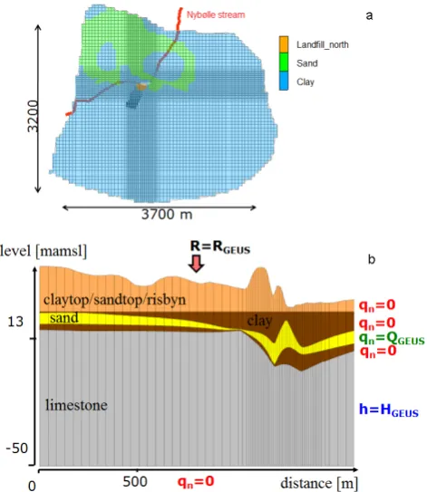
Fig. 2 Groundwater model (a), where red crosses mark head observations, black arrows represent the flux observations used for the 2
JHI and SHI. The TDEM model (b) comprises a 1D, 2-layer electrical resistivity model. 3
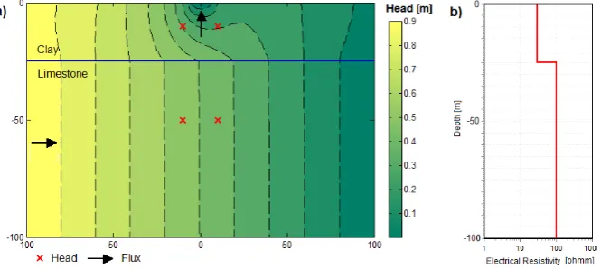
Fig. 2. Groundwater model (a), where red crosses mark head observations, black arrows represent the flux observations used for the JHI and
SHI. The TDEM model (b) comprises a 1-D, 2-layer electrical resistivity model.
2.3 Implementation
The SHI and JHI are applied for two cases. The first case combines a synthetic groundwater model and a synthetic TDEM data set. The second case combines a real-world groundwater model and a field ERT data set.
To generate the geophysical forward responses for the TDEM and ERT, EM1DINV (HGG, 2008) is used. EM1DINV is also used to generate a forward response for the ERT data (Auken and Christiansen, 2004). The geophys-ical model that is estimated for the TDEM is a 1-D resistivity model (Fig. 2b), in which typically a number of layer thick-nesses and layer resistivities are estimated. For the ERT data, neighboring 1-D resistivity models (Fig. 8a) are tied together by lateral constraints (Auken and Christiansen, 2004).
The groundwater model in the synthetic example is im-plemented in Matlab (PDE-tool). For the real-world model MODFLOW (Harbaugh et al., 2000) is used. More details about the groundwater models and geophysical data are given in the next section.
3 Example 1: synthetic study TDEM
3.1 Setup
The first application of the JHI and SHI considers a synthetic cross-sectional groundwater model and a TDEM sound-ing. As part of the geophysical inversion a TDEM forward model is used. This forward model is based on Ward and Hohmann (1988) and includes the modeling of low-pass fil-ters (Efferso et al., 1999) and the turn-on and turn-off ramps described in Fitterman and Anderson (1987).
The groundwater model in the synthetic example consists of two layers, similar to the geological setup of the field study we discuss in Sect. 4. The upper layer, with a thicknessDclay,
is considered to be clayey sand with hydraulic conductivity
Kclay [m s−1]. The second layer represents limestone with
hydraulic conductivityKlime. Different values are generated for these properties as will be explained below. Constant heads are applied as boundary conditions (right: 1 m; left: 0 m); in the middle of the model domain a river is assumed to be located with a fixed head of 0. This results in flow from left to right and flow towards the river. From this realization we extract a number of groundwater observations, compris-ing 4 head and 2 flux measurements that are shown in Fig. 2a. The groundwater parameters (γ )that need to be estimated in-clude the hydraulic conductivity of the limestone (Klime)and
the clay (Kclay)and the thickness of the clay (Dclay). Due
to the parameter cross-correlation betweenKclay andDclay,
an additional flux measurement for the limestone is included, which is not available for most real-world modeling studies. TypicallyDclayis not estimated when calibrating a ground-water model, due to its correlation withKclay. This parameter was chosen to illustrate the use of a JHI and SHI, in which the hydrostratigraphy of a groundwater model is coupled with a geophysical model.
For the synthetic study we assume the availability of one TDEM sounding. The parameters of the geophysical model (π )that are estimated comprise one layer thickness (t1) and
electrical resistivities for layer 1 and 2 (r1 and r2) using
30 synthetic apparent resistivity observations. The simplified 1-D description of the geophysical model is used because of the negligible effect of the water table variation and unsatu-rated zone thickness in the model, compared to the geometry of the model and the TDEM resolution.
[image:7.595.133.466.68.217.2]Table 1. Model properties used in the synthetic example.
Model Property Value
Constant Head (west) [m] 1 Constant Head (east) [m] 0 Constant Head (river) [m] 0 Error Head Measurements [m] 0.02 Error Flux Measurements [ %] 30
Error TDEM Measurements [ %] ca. 3 %; based on a real sounding
Table 2. Coupling constraints standard deviations,ec, used for JHI Runs 1–7.
Constraint Equation Run 1 Run 2 Run 3 Run 4 Run 5 Run 6 Run 7
Petrophysical Log10(Kclay)−Log10(r1)+6 3 2 1 0.5 0.3 0.1 0.05
Geometric Dclay−t1 7 5 2 1 0.5 0.1 0.05
mean values of respectively−5 and 25 m with a standard de-viation of respectively 0.1 and 0.1 m. Subsequently values of
r1andt1are generated based on the equations in the second
column of Table 2, including a random component with a standard deviation,ecorr, that defines the level of correlation between the geophysical and groundwater model parameters. Measurement error is then added to the simulation results of each parameter realization, employing a standard devia-tion (eh)of±2 cm for the head observations and±30 % for the flux measurements. The measurement errors added to the TDEM data have a standard deviation (eg)of ca.±3 % of the measurement value and are based on a real-world TDEM sounding.
The TDEM measurement error does not only reflect the standard deviation of the data stack and includes an addi-tional error component to take into account 3-D effects and imperfect instrument specifications (e.g., filters, wave form of the applied pulses). This additional error component will typically yield correlated measurement errors. For example, Efferso et al. (1999) provide the effect of different low pass filters on the TDEM forward response. In this research, how-ever, we do not investigate correlated errors and thus add un-correlated measurement error to the TDEM data to be con-sistent with the Gaussian assumptions of least-squares inver-sion theory (Tarantola, 2005). Different starting parameters are used for the calibration of the geophysical and ground-water model with each observation realization.
3.2 Geometric and petrophysical relationship
To perform the JHI and SHI two types of constraints are em-ployed between the groundwater and TDEM model, a geo-metric and a petrophysical constraint. Both relationships are defined in Table 2. The geometric constraint applies to the depth of the clay layer (Dclay)and the thickness of the first layer in the TDEM model (t1).
The petrophysical coupling constraint applies to the hy-draulic conductivity of the upper layer of the groundwater model (Kclay)and the electrical resistivity of the first layer in
the TDEM model (r1). This constraint applies a relationship
between the logarithmic values of hydraulic conductivity and electrical resistivity (Niwas and de Lima, 2003; Slater, 2007). The petrophysical relationship in Table 2 was arbitrarily cho-sen, but implies a decreasing hydraulic conductivity for a de-creasing electrical resistivity, as hydraulic conductivity and electrical resistivity decrease for increasing clay content. A typical hydraulic conductivity for clay is 10−5m s−1(Fetter,
1994) and 101m is a representative electrical resistivity (Kirsch, 2006), which results in an expected value of−6 for the petrophysical coupling constraint. Note that this is an ex-tremely simplified relationship between hydraulic conductiv-ity and electrical resistivconductiv-ity.
In a first configuration of the synthetic study, we generate realizations of “true” parameters, using a standard deviation (ecorr)of 0.01 for the petrophysical relationship and a
stan-dard deviation 0.05 (ecorr)for the geometric relationship. In a second configuration, we apply largerecorrvalues of respec-tively 0.1 and 0.1. As the parameter coupling in the SHI can be very strong for well-resolved geophysical parameters, this second configuration is used to test whether or not the SHI results in worse groundwater parameter estimates when cor-relation between groundwater and geophysical parameters is relatively weak.
3.3 SHI
The SHI starts with a geophysical inversion for the TDEM data after which the estimated electrical resistivity model,
πest, is used as an observation in the calibration process of
the groundwater model. In this case πestcomprises the
es-timated values fort1andr1, which we employ to constrain
the groundwater model parametersDclay andKclay. For the
[image:8.595.87.509.209.254.2]1 2 3 4 5 6 7 0
20 40 60 80 100 120
strength coupling (1: weak - 7: strong)
error K
cl
ay
[%
]
1 2 3 4 5 6 7
0 20 40 60 80 100
strength coupling (1: weak - 7: strong)
er
ro
r K
lim
e
[%]
1 2 3 4 5 6 7
0 10 20 30 40
strength coupling (1: weak - 7: strong)
error D
cl
ay
[%
]
1 2 3 4 5 6 7
0 5 10 15 20 25 30
strength coupling (1: weak - 7: strong)
er
ro
r r1
[%
]
1 2 3 4 5 6 7
0 50 100 150 200 250
strength coupling (1: weak - 7: strong)
er
ro
r r2
[%
]
1 2 3 4 5 6 7
0 10 20 30 40
strength coupling (1: weak - 7: strong)
er
ro
r t1
[%
]
[image:9.595.55.549.66.328.2]1
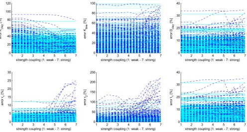
Fig. 3 Parameter errors for JHI Run 1-7 for 250 realizations and increasing weight for the coupling constraints (blue dashed lines). The
2
cyan lines indicate the parameter errors for the 250 SHI runs. Groundwater model parameters are shown in the upper row of figures,
3
geophysical parameters on the bottom row. Standard deviations of the JHI coupling constraints, e
c, are listed in Table 2.
4
5
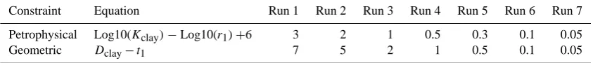
Fig. 3. Parameter errors for JHI Runs 1–7 for 250 realizations and increasing weight for the coupling constraints (blue dashed lines). The cyan
lines indicate the parameter errors for the 250 SHI runs. Groundwater model parameters are shown in the upper row of figures, geophysical parameters on the bottom row. Standard deviations of the JHI coupling constraints,ec, are listed in Table 2.
recommendes values of 10−2–10−1for coupling hydraulic
conductivities and well-resolved electrical resistivities and values of 101–102for poorly resolved electrical resistivities. We employ values based on the posterior standard deviation of the geophysical parameters, obtained with the geophysical inversion, to honor the resolution level of parameters inferred from geophysical data and constraints.
For the SHI, the second line in Eq. (13) becomes
1 0 0 0 0 1
log 10(Kclay) Klime Dclay
=
log 10(r1)−6
t1
+es. (25)
AsKlimeis not constrained with the geophysical inversion
results, its associated entries (matrix Ps, Eq. 13) are 0.
3.4 JHI
For the JHI we use the same type of coupling constraints for the same geophysical and hydrological parameters. However, now the geophysical parameters are also part of the inversion and Eq. (18) is used for the coupling constraints. For this application Eq. (18) becomes
1 0 0−1 0 0 0 1 0 0 −1 0
log 10(r1) t1 t2
log 10(Kclay) Klime Dclay
=
6 0
+ec, (26)
where the expected value for the geometric constraint be-tweenDclay andt1is 0, whereas the petrophysical
relation-ship between log10(Kclay)and log10(r1)is 6. The JHI is
un-dertaken for varying values of ec, as defined by the values
in Table 2. This range is comparable with the recommended range foresin Dam and Christensen (2003).
The value ofec reflects the strength of the coupling
rela-tionship. Anecof 0.01 means the assumed error of the
cou-pling relationship has a standard deviation of 0.01, marking a strong coupling relationship compared to an implementa-tion employing andecof e.g., 10. For the synthetic study the weight associated with the coupling constraints is varied, by changing this standard deviation. Table 2 lists 7 different con-figurations of JHI (referred to as “Runs”) employing different
ecvalues to increase the weight for the coupling relationship
between Dclay [m] and t1 [m] and the coupling constraint
between log10(Kclay)[m d−1] and log10(r1)[m]. For the
petrophysical constraintecis varied from 3 to 0.05; for the
0 1 2 0 50 Cou nt RMSE Heads
0 1 2
0 50
Cou
nt
RMSE Heads
0 1 2
0 50
Cou
nt
RMSE Heads
0 1 2
0 50
Cou
nt
RMSE Heads
0 1 2
0 50
Cou
nt
RMSE Flux
0 1 2
0 50
Cou
nt
RMSE Flux
0 1 2
0 50
Cou
nt
RMSE Flux
0 1 2
0 50
Cou
nt
RMSE Flux
0 1 2
0 50
Cou
nt
RMSE Geophysics
0 1 2
0 50
Cou
nt
RMSE Geophysics
0 1 2
0 50
Cou
nt
RMSE Geophysics
0 1 2
0 50
Cou
nt
RMSE Geophysics
0 0.1 0.2
0 100 200
C
ount
RMSE Geom. con.
0 0.1 0.2
0 100 200
C
ount
RMSE Geom. con.
0 0.1 0.2
0 100 200
C
ount
RMSE Geom. con.
0 0.1 0.2
0 100 200
C
ount
RMSE Geom. con.
0 0.1 0.2
0 100 200 Co un t
RMSE Petro. con.
0 0.1 0.2
0 100 200 Co un t
RMSE Petro. con.
0 0.1 0.2
0 100 200 Co un t
RMSE Petro. con.
0 0.1 0.2
0 100 200 Co un t
RMSE Petro. con.
JHI Run 1
JHI Run 4
JHI Run 7
SHI
1
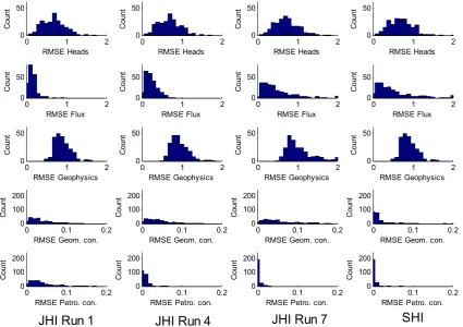
Fig. 4 Histograms of data fit for the different components of the objective function in JHI Run 1, 4 and 7. Results are for 250
2
realizations. The last column shows data fit for the SHI.
3
4
Fig. 4. Histograms of data fit for the different components of the objective function in JHI Runs 1, 4 and 7. Results are for 250 realizations.
The last column shows data fit for the SHI.
were chosen to cover a JHI with weak coupling constraints and a JHI assumingecvalues of similar magnitude compared
to the standard deviations,ecorr, that were used for generating
the correlated “true” parameters. 3.5 Results
First a JHI is conducted for the groundwater and the geophys-ical model. This was done using 250 observation realizations and different parameter starting values. 7 JHI simulations are performed using an increasing strength of coupling between the TDEM and groundwater model (Runs 1–7). To generate correlated “true” geophysical and groundwater model param-eters, standard deviationsecorr of 0.01 and 0.05 are respec-tively used for the petrophysical and geometric constraint.
Run 1 represents a JHI with a very small weight (i.e., large
ec)for the coupling constraints representing an independent inversion in which the groundwater model is not informed with the TDEM model and vice versa. Figure 3 shows all the parameter estimates pertaining to the JHI Run 1–7 for 250 re-alizations, expressing how well parameter estimates compare with the “true” parameter values that were generated. Param-eter errors in Fig. 3 are given as a percentage with respect to the “true” parameter value. For JHI Run 1 parameter errors are up to 100 % forKclayandKlimeand up to 40 % forDclay.
Geophysical parameterr1is well-resolved and shows errors
of less than 7 %.t1andr2show errors of respectively 40 and
200 %.
The strength of the coupling constraints is subsequently increased using smaller values forec(Table 2) in JHI Runs
2–7. The blue dashed lines in Fig. 3 shows how parameter es-timates react as a result of the stronger coupling constraints. A large and rapid reduction of error can be observed forKclay
showing an error decrease from 100 % to about 10 %. Esti-mates forDclaydo not improve and errors remain at a value of up to about 40 %. Geophysical parameter errors are fairly constant for Runs 1–7, except for a slightly increasing num-ber of realizations showing larger errors for parameterr1and
t1in JHI Runs 6 and 7 in which the coupling constraints have
the largest weight.
[image:10.595.86.512.67.367.2]1 2 3 4 5 6 7 0
20 40 60 80 100 120
strength coupling (1: weak - 7: strong)
er
ro
r K
cl
ay
[%
]
1 2 3 4 5 6 7
0 20 40 60 80 100
strength coupling (1: weak - 7: strong)
erro
r K
lim
e
[%
]
1 2 3 4 5 6 7
0 10 20 30 40
strength coupling (1: weak - 7: strong)
er
ro
r D
cl
ay
[%
]
1 2 3 4 5 6 7
0 5 10 15 20 25 30
strength coupling (1: weak - 7: strong)
erro
r r1
[%
]
1 2 3 4 5 6 7
0 50 100 150 200 250
strength coupling (1: weak - 7: strong)
erro
r r2
[%
]
1 2 3 4 5 6 7
0 10 20 30 40
strength coupling (1: weak - 7: strong)
erro
r t1
[%
]
[image:11.595.52.549.64.330.2]1
Fig. 5 Error parameter estimates for the second configuration of JHI and SHI runs using 250 parameter realizations and larger e
corrfor
2
the generated “true” parameters. Blue dashed lines indicate parameter errors for JHI Run 1-7, where the cyan lines indicate the
3
parameter errors for the SHI.
4
5
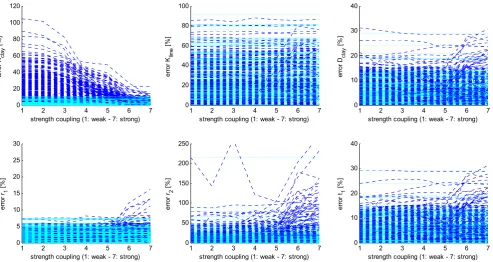
Fig. 5. Error parameter estimates for the second configuration of JHI and SHI runs using 250 parameter realizations and largerecorrfor the
generated “true” parameters. Blue dashed lines indicate parameter errors for JHI Runs 1–7, where the cyan lines indicate the parameter errors for the SHI.
of the petrophysical coupling constraint due to the employed weighting strategy and the high parameter sensitivity ofr1
that is subjected to this constraint.
Secondly, a SHI is applied to evaluate the performance of the JHI. The cyan lines in Fig. 3 show the parameter errors for the SHI. These results show a large reduction in parameter error forKclayandDclaycompared to JHI Run 1. For
param-eterKclaythis reduction of error is similar to JHI Runs 6 and
7. ForDclaythe SHI performs better compared to JHI Runs 6
and 7, indicated by the number of JHI realizations with an er-ror larger than 15 %. Compared to these runs the geophysical parameter errors are generally smaller for the SHI. The last column in Fig. 4 lists the data fit for the SHI. As the inverted TDEM models of JHI Run 1 are used in the SHI, the his-togram for the TDEM data is identical to that of the TDEM data in JHI Run 1. Head and flux data are fitted less well compared to JHI Run 1. The fit for both coupling constraints indicate a relatively strong petrophysical constraint.
Finally, a second configuration of JHI and SHI is tested in which a larger standard deviation (ecorr)was used to
gen-erate less correlated parameter realizations forKclay,Dclay, r1andt1; 0.1 for the petrophysical constraint and 0.5 for the
geometric constraint. Figure 5 shows a reduction in param-eter error forKclay compared to JHI Run 1 from about 100
to 60 %. The SHI resulted in a similar reduction. The im-provement inKclay, however, is much smaller compared to the results in Fig. 3. Geophysical parametersr1andr2in JHI
Runs 6 and 7, show worse estimates compared to JHI Runs 6 and 7 in Fig. 3.
The average computational burden associated with the in-version for a single realization was 94 (61+33) model calls for the SHI compared to 306 (153+153) model calls for the JHI. As the estimation of geophysical and groundwater model parameters is conducted simultaneously, the number of iterations in which geophysical and groundwater model parameters are updated are the same, which is not the case in a SHI. This will result in a larger computational burden for the JHI.
4 Example 2: case study Risby landfill
As second example we consider a steady-state, real-world groundwater model for Risby landfill located in Denmark, to which we refer as the Risby model. This model was de-veloped by Christensen and Balicki (2010) to characterize the hydrogeological interaction between a landfill, a local stream and a regional aquifer that is used for water supply. Christensen and Balicki (2010) provide a thorough descrip-tion and discussion of the assumpdescrip-tions underlying the setup of this model and its results.
1
Fig. 6 An aerial overview of Risby landfill, the ERT profile, parameter PP1 and available boreholes and hydrogeological observation
2
data at Risby landfill.
3 Fig. 6. An aerial overview of Risby landfill, the ERT profile,
param-eter PP1 and available borehole and hydrogeological observation
data at Risby landfill.
Risby area and the Risby groundwater model, after which we conduct a simple linear sensitivity analysis for the differ-ent hydrogeological parameters in the groundwater model, followed by the application of a SHI and JHI to inform the groundwater model with the ERT data.
4.1 Description of Risby landfill
An extensive historical overview of Risby landfill was pro-vided by Thomsen et al. (2011). Figure 6 lists the key fea-tures of the study area, which are a landfill and a small brook called Nybølle stream. The geological setting of Risby landfill (Højberg et al., 2008; CarlBro, 1988) comprises pre-Quaternary limestone bedrock overlain by pre-Quaternary glacial deposits. The pre-Quaternary limestone surface is located be-tween−10 and+5 m a.m.s.l., corresponding to 20–30 m be-low the natural terrain surface. The Quaternary glacial de-posits mainly consist of clay till, but intercalated sand lenses and sand layers are common. The sandy deposits range in thickness from a few centimeters to several meters.
4.1.1 Groundwater model
Figure 7a shows the horizontal grid discretization that is used to simulate groundwater levels near Risby landfill. The grid cell size employed in the groundwater model is 50 m by 50 m. Near the landfill a smaller cell size of 12.5 m by 12.5 m is em-ployed. For the geological setup, 5 continuous layers were chosen, where the 4 upper layers represent the sand and clay layers of the glacial clay till and the lowest layer represents the field-scale limestone aquifer. The top layer of the model, with its bottom elevation fixed at+15 m a.m.s.l. was subdi-vided in 3 zones, which represent the extent of the upper sandy and clayey deposits together with the delineation of the northern part of the landfill (Fig. 7a).
[image:12.595.312.548.66.338.2]1 2
Fig. 7 Horizontal discretization of the Risby groundwater model and zonation of layer 1 (a) and the geological setup and boundary 3
conditions used (b). 4
Fig. 7. Horizontal discretization of the Risby groundwater model
and zonation of layer 1 (a) and the geological setup and boundary conditions used (b).
Boundary conditions applied in the Risby model are shown in Fig. 7b and consist of constant heads, derived from a regional groundwater model, referred to as the GEUS-model (Højberg et al., 2008). The limestone was assumed to be impermeable at a level of −50 m a.m.s.l. and a no flow boundary was therefore assigned. The boundaries for the top layer and the remaining two clay layers were also set as no flow boundaries. The symbolsQGEUS,HGEUSand
RGEUSindicate the specified flux, constant head values and
recharge, which were extracted from the regional GEUS-model. Boundaries for the limestone were set as constant head boundaries with a hydraulic head equal to 14.9 m. The isopotential used, was the average simulated head in the limestone for the period 2001–2005 (Højberg et al., 2008). Boundaries for the sand layer were prescribed flux bound-aries. A flux of 7.2×10⁻⁶m3s−1 was applied for all cells along the boundary.
Table 3. Inversion results JHI and SHI for Risby landfill.
Inversion result CHI (ec=0.2) SHI Separate_Inversion
Log10K_clay [m d−1] −7.79±0.19 7.54±0.16 −7.52±0.19 Log10K_sand [m d−1] −3.96±0.47 −4.26±0.38 −4.25±0.44 Log10K_lime [m d−1] −3.85±0.04 −3.96±0.14 −3.99±0.66 Log10K_risbyn [m d−1] −2.20±0.16 −2.33±0.01 −2.39±0.63 Log10K_claytop [m d−1] −5.93±0.33 −5.81±0.35 −5.80±0.25 Log10K_sandtop [m d−1] −4.35±0.33 −4.43±0.33 −4.42±0.01 PP1[m] 26.58±0.57 28.03±0.99 28.26±0.54
Average thick1, model 14–16 [m] 4.53±3.08 4.55±2.95 4.55±2.95 Average thick2, model 14–16 [m] 20.16±3.94 20.22±3.98 20.22±3.98 Average Log10 res1, model 1–10 [m] 1.02±0.10 1.01±0.08 1.01±0.08 Average Log10 res2, model 1–10 [m] 1.44±0.46 1.88±0.54 1.88±0.54
Groundwater model runs 210 63 91
Geophysical model runs 3230 1520 1520
Misfit geophysicsφg 0.80 0.79 0.79
Misfit hydrogeologyφh 0.76 0.70 0.65
4.1.2 ERT data
The landfill and its surroundings were mapped using various geoelectrical profiles for which ERT and induced polariza-tion data (Slater, 2007) were collected in order to delineate the landfill, sand pockets and the thickness of the glacial de-posits overlying the limestone aquifer (Gazoty et al., unpub-lished data). To demonstrate the SHI and JHI, we used the data associated with one of these ERT profiles north of the landfill; the location of the profile is shown in Fig. 6.
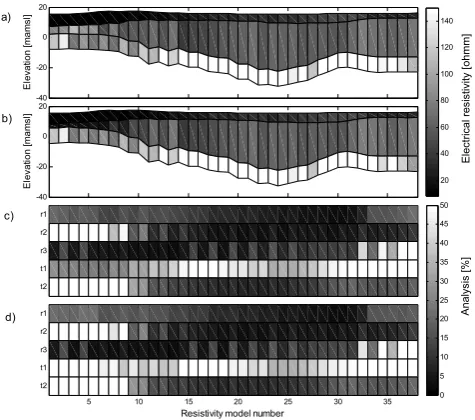
Figure 8a shows the inverted resistivity model for the ERT profile using a few-layer, laterally constrained inversion (LCI) approach as discussed in Sect. 2.1. This ERT profile consists of 37 1-D resistivity models with 3 layers and is ori-entated west–east (model number 0 marks the western point). The parameters estimated for each of the 37 resistivity mod-els (5 m spaced) comprise 3 layer resistivities (r1,r2andr3)
and 2 layer thicknesses (t1andt2). Lateral constraints were
used with a weight factor of 1.2 for the layer depths (CRh)
and a weight factor of 1.2 for the resistivities between neigh-boring resistivity models. These weight factors are described in Auken and Christiansen (2004) and their value is subjec-tively determined and based on common practice ranges sug-gested in HGG (2008).
At the location of the ERT profile, boreholes showed a de-pression in the limestone surface down to ca.−10 m a.m.s.l. This depression has been interpreted as a buried paleoval-ley in the pre-Quaternary landscape and its shape is not well captured with the available boreholes. Another characteristic are relatively thick sand layers at the eastern part of Risby landfill.
In Fig. 8a the limestone shows up as a bottom layer of relatively resistive material of ca. 100–150m, which dips down towards the east. Sandy deposits are more abundant at the eastern part of the landfill as evidenced by the relatively
-40 -20 0 20
E
lev
at
ion [
m
am
sl
]
r1
r2
r3
t1
t2 -40 -20 0 20
E
levat
io
n
[m
am
sl
]
0 5 10 15 20 25 30 35 40 45 50
5 10 15 20 25 30 35
r1
r2
r3
t1
t2
Resistivity model number
20 40 60 80 100 120 140
a)
Analys
is [%]
El
ectrica
l res
istivity [oh
mm]
b)
c)
d)
1
Fig. 8 Inverted ERT model obtained after a separate geophysical inversion (a) and using the JHI with ec=0.2 (b) together with a
2
parameter uncertainty analysis expressed by their standard deviation relative to the parameter estimate. A gray scale marks well (dark 3
colored) and undetermined parameters (light colored) for the separate geophysical inversion (c) and a JHI with ec=0.2 (d).
4 5
Fig. 8. Inverted ERT model obtained after a separate geophysical
inversion (a) and using the JHI withec=0.2 (b) together with a
pa-rameter uncertainty analysis expressed by their standard deviation relative to the parameter estimate. A gray scale marks well (dark colored) and undetermined parameters (light colored) for the sepa-rate geophysical inversion (c) and a JHI withec=0.2 (d).
[image:13.595.310.548.301.511.2]0 0.1 0.2 0.3 0.4 0.5 0.6 0.7
Kclay Ksand Klime Krisbyn Kclaytop Ksandtop PP1
Sc
a
le
d
S
e
n
sit
iv
it
ie
s
[
‐
]
[image:14.595.49.284.65.190.2]1
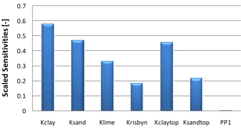
Fig. 9 Scaled Sensitivities for the parameters of the Risby model.
2 Fig. 9. Scaled sensitivities for the parameters of the Risby model.
(Milosevic et al., 2012). Figure 8c shows the uncertainty as-sociated with the parameters that are estimated in the ERT model, expressed by their standard deviation as a percentage of the parameter estimate. This parameter uncertainty anal-ysis included all the information provided by the data and parameter constraints. Note light colors in Fig. 8c indicate relatively poorly resolved parameters, e.g.,r1,r2andt1 for
models 1–10.
4.2 Informing the Risby model with ERT data
As mentioned before, 6 parameters are estimated in the orig-inal Risby model (Christensen and Balicki, 2010), which are listed in Table 3. For these parameters a local, linear sensi-tivity analysis (Fig. 9) is conducted using PEST (Doherty, 2010). This analysis shows that the hydraulic conductivity pertaining to the clay layer (Kclay)is the most sensitive pa-rameter.
To improve the estimate ofKclaya petrophysical relation-ship is applied, which is used in Eqs. (25) and (26). An expected value of 9 is used, as clay till has an approxi-mate hydraulic conductivity of 10−8m s−1(Fredericia, 1990; CarlBro, 1988) and an electrical resistivity of about 101m (Kirsch, 2006). This relationship implies a higher electrical resistivity is accompanied by a smaller clay content, which, in turn, results in a higher hydraulic conductivity.r1andr2in
resistivity model numbers 1–10 are coupled to the estimation
ofKclay, as the area eastern part of the ERT profile (model
numbers 15–37) contains large sandy deposits embedded in the clay. As we are only using a 3 layer resistivity model the average electrical resistivity in this part of the domain would not reflect the resistivity of the clay appropriately.
As the ERT model also informs about the depth to the limestone, we introduce an additional parameter (PP1) in
the groundwater model representing the top elevation of the limestone. PP1represents a single pilot point (Certes and
De-marsily, 1991) used to interpolate the elevation of the lime-stone surface together with the available borehole informa-tion. The location of PP1, which is shown in Fig. 6, is picked
as the depression of the limestone surface, occurring at the northeastern part of the landfill, is not well characterized. As
expected, the calculated sensitivity, based on Hill (1998), of this parameter is very small with respect to the hydrogeo-logical observations (Fig. 9). To demonstrate the effect of geometric coupling we use parameter PP1 in the inversion
process. Parameterst1 andt2 in model numbers 14, 15 and
16 are coupled to the estimation of PP1.
4.3 SHI
The SHI starts with the estimated geophysical model shown in Fig. 8a. The scale of the individual 1-D resistivity mod-els comprised by the ERT model is rather small (electrode spacing of 5 m) compared to the grid cell size of 12.5 m used in the groundwater model. For this purpose we have chosen to constrainKclaywith the average electrical resistivity es-timates,r1 and r2, pertaining to resistivity model numbers 1–10. To constrain the estimation of PP1we use the average
sum oft1andt2pertaining to resistivity model numbers 14, 15 and 16. The weights associated with the constraints were based on the standard deviations of the geophysical parame-ter estimates calculated using Eq. (7).
4.4 JHI
We also apply a JHI for the Risby model to estimater1,r2
andKclay using the petrophysical relationship described in
Sect. 4.2. For the estimation of the depth to the limestone we introduce a geometric coupling constraint between parame-ters PP1,t1andt2. The petrophysical coupling constraint is
used for resistivity models 1–10, the geometric constraint for resistivity models 14, 15 and 16.
4.5 Results
The last column in Table 3 shows the parameter estima-tion results for a separate inversion of both the geophysical and the groundwater model. Most of the parameters in the groundwater model are estimated with relatively small pos-terior standard deviation. When performing a SHI (Table 3, column 2), the decrease in parameter uncertainty is negligi-ble except forKlimeandKrisbyn. Parameter estimates remain
similar to the separate inversion, which is likely caused by the large standard deviations associated with the geophysical parameters that are coupled with the groundwater model. In Fig. 8c these parameters show a relatively large standard de-viation. As we used this standard deviation to determine the weight of the constraints in the SHI, the constraint might be too weak to affect the estimation of the groundwater model parameters significantly.
Figure 10 shows the parameter estimates and 68 %-confidence intervals for the JHI, when using different weight values for the coupling constraints (ec). The parameter
esti-mates forKclay andr2 are affected when the weight of the
petrophysical relationship is increased by setting the accept-able error ec to a smaller value. The geometric constraint
1
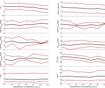
Fig. 10 Parameter estimates (black straight line) and confidence bounds (red dashed lines) for different values of ec when performing a
2
JHI using a petrophysical relationship between Kclay, r1 and r2 and a geometrical constraint between parameters PP1 and t1 and t2. The
3
confidence bounds represent the parameter estimate ± 2 standard deviations. 4
5 6
Fig. 10. Parameter estimates (black straight line) and confidence bounds (red dashed lines) for different values ofec when performing a
JHI using a petrophysical relationship betweenKclay,r1andr2and a geometrical constraint between parameters PP1andt1andt2. The
confidence bounds represent the parameter estimate±2 standard deviations.
estimated values of the geophysical parameters. However the estimate of PP1 does approximate the geophysical model
better when the constraint is given more weight. The aver-age depth to the limestone in the ERT model is about 25 m (t1+t2). In the groundwater model, this depth is estimated to be 28.3 m±0.5 and 28.0 m±1.0 m using a separate inver-sion and a SHI, respectively. In the JHI this estimate becomes ca. 26.6 m±0.6 m. Table 3 shows that standard deviations of the groundwater model parameters for the JHI are almost equivalent compared to the SHI, but smaller compared with a separate inversion.
The main advantage of the JHI is seen from the estimated values for the geophysical parameters that are allowed to change in the JHI. Geophysical layer thicknesses,t1andt2,
decrease slightly compared with the SHI, while electrical re-sistivityr2shows a more significant change.
Figure 8b is the inverted ERT model using the JHI with an
ecof 0.2. Compared with the geophysical inversion results in
Fig. 8a the estimated resistivity of layer 2 dropped from an average of 75 to ca. 30m for resistivity models 1–10. These are the models for which electrical resistivitiesr1andr2were coupled toKclayin the groundwater model. Figure 8d shows the standard deviations associated with the estimated geo-physical model obtained with the JHI. The standard deviation
of parameterr2indicates it is not well determined using the JHI as was the case in the separate geophysical inversion.
r1is determined with an approximate standard deviation of 10 %. However, Fig. 8d showst1 is less well resolved for those model numbers where the petrophysical relationship is applied. The geometric coupling constraint does not show any effect on the estimated geophysical models in Fig. 8.
Table 3 lists the RMSE with respect to the geophysical and hydrogeological observations (respectivelyϕg andϕh),
which was smaller than 1 for all simulations. No significant increase in data fit was noted, except a slightly higher ϕh
for the JHI. Increasing the weight of the coupling constraints (by decreasingec)or increasing the number of coupling
con-straints, will ultimately result in an increase inϕgandϕh, as
the geophysical and groundwater data will pull parameters in different directions.
[image:15.595.122.477.62.358.2]5 Discussion and conclusions
This study tested a SHI and a new type of JHI for a ground-water model and different types of geophysical data. The JHI estimated geophysical and groundwater parameters si-multaneously, employing coupling constraints acting as ad-ditional regularization terms to exploit potential correlation between geophysical and hydrogeological properties that can be based on established petrophysical relationships. The SHI employed similar coupling constraints, but included an inde-pendent geophysical inversion. The weight of the SHI cou-pling constraints was based on geophysical parameter reso-lution.
Both the SHI and JHI approaches can provide consistent inversion frameworks and offer a high level of flexibility when coupling groundwater and geophysical models because 1. only selected geophysical model parameters can be
coupled to groundwater model parameters,
2. confidence associated with the hydrological interpre-tation of a geophysical model can be tuned using dif-ferent weights for the employed coupling constraints, 3. scale issues can be overcome by coupling several
geo-physical parameters to hydrological parameters or vice versa,
4. SHI and JHI can be applied for various combinations of geophysical methods and groundwater models, and 5. SHI and JHI can be used with other types of optimiza-tion methods (e.g., Markov–Chain Monte Carlo meth-ods) by adding an additional coupling constraint com-ponent to the objective function that is minimized. Furthermore, the JHI and SHI are consistent with state-of-the-art inversion techniques used for groundwater models, resistivity and airborne electromagnetic data.
For a synthetic study, comprising a cross-sectional ground-water model and TDEM data, a JHI and SHI resulted in im-proved parameter estimates and a reduction in parameter un-certainty in comparison with a groundwater model that is not informed with TDEM data. Groundwater parameter esti-mates using a JHI did not improve compared with a SHI and resulted in slightly worse parameter estimates for the geo-physical model when using large weights for the coupling constraints. A second configuration of the synthetic study, incorporating lower quality (petro)physical relationships be-tween geophysical and groundwater parameters resulted in decreasing performances for both the SHI and JHI. The SHI performed slightly better compared to the JHI based on the geophysical parameter estimates and geophysical data mis-fit. In contrast to the JHI, the SHI overestimated the level of correlation between geophysical and groundwater param-eters. To avoid overestimating model coupling strength in a SHI (which can result in an underestimation of parame-ter uncertainty), weighting strategies for parameparame-ter coupling
constraints should be based on that element (parameter res-olution or petrophysical relationship) that incorporates the largest error.
For the case of a real-world, field-scale groundwater model and an ERT section, parameter uncertainty was significantly decreased for two parameters in the groundwater model us-ing both a JHI and SHI. The JHI resulted in different param-eter estimates for both the groundwater and the geophysical model, honoring the imposed coupling constraints. Parame-ter uncertainty was not reduced in comparison with a SHI.
For the cases investigated in this paper the SHI proves to be more useful based on analyses of parameter estimates and data fit. In addition, the JHI requires a 2–3 times larger com-putational burden and is relatively difficult to implement. The JHI might still be useful when groundwater and geophysical models can mutually benefit from differences in parameter resolution. For coupling geophysical models with field-scale or regional groundwater models, such situation is not likely to occur as the groundwater models are relatively more prone to conceptual errors and limited observation data. Finally, when planning hydrogeophysical surveys and modeling, pa-rameter sensitivity studies are of crucial importance to ex-plore parameters that need to be determined, given targeted groundwater model predictions, and to determine whether parameter resolution in geophysical models provides oppor-tunities to constrain these parameters.
Acknowledgements. This work was conducted at the Technical University of Denmark and supported by the Danish Agency for Science Technology and Innovation funded project RiskPoint – Assessing the risks posed by point source contamination to groundwater and surface water resources under grant number 09-063216. We also like to thank Monika Balicki and Mette Christensen for the main development of the Risby groundwater model and Aurélie Gazoty for the ERT data collection. Finally, we want to thank three anonymous reviewers for sharpening a previous version of this paper.
Edited by: G. Fogg
References
Archie, G. E.: The electrical resistivity log as an aid in determin-ing some reservoir characteristics, Transactions of the American Institute of Mining and Metallurgical Engineers, 146 154–161, 1942.
Auken, E. and Christiansen, A. V.: Layered and laterally con-strained 2d inversion of resistivity data, Geophysics, 69, 752– 761, doi:10.1190/1.1759461, 2004.
Bauer-Gottwein, P., Gondwe, B. N., Christiansen, L., Herckenrath, D., Kgotlhang, L., and Zimmermann, S.: Hydrogeophysical ex-ploration of three-dimensional salinity anomalies with the time-domain electromagnetic method (tdem), J. Hydrol., 380, 318– 329, doi:10.1016/j.jhydrol.2009.11.007, 2010.