Accepted Manuscript
Model-driven engineering of planning and optimisation algorithms for
pervasive computing environments
Anthony Harrington, Vinny Cahill
PII:
S1574-1192(11)00125-8
DOI:
10.1016/j.pmcj.2011.09.005
Reference:
PMCJ 300
To appear in:
Pervasive and Mobile Computing
Please cite this article as: A. Harrington, V. Cahill, Model-driven engineering of planning and
optimisation algorithms for pervasive computing environments,
Pervasive and Mobile
Computing
(2011), doi:10.1016/j.pmcj.2011.09.005
Model-Driven Engineering of Planning and Optimisation Algorithms for
Pervasive Computing Environments
Anthony Harringtona,∗, Vinny Cahillb
aDistributed Systems Group, Trinity College Dublin, and Faculty of Mathematics, Informatics and Mechanics, University of Warsaw. bDistributed Systems Group, Lero - The Irish Software Engineering Centre, School of Computer Science and Statistics, Trinity College Dublin.
Abstract
This paper presents a model-driven approach to developing pervasive computing applications that exploits design-time information to support the engineering of planning and optimisation algorithms that reflect the presence of uncertainty, dynamism and complexity in the application domain. In particular the task of generating code to implement planning and optimisation algorithms in pervasive computing domains is addressed.
We present a layered domain model that provides a set of object-oriented specifications for modelling physical and sensor/actuator infrastructure and state-space information. Our model-driven engineering approach is implemented in
two transformation algorithms. The initial transformation parses the domain model and generates a planning model for the application being developed that encodes an application’s states, actions and rewards. The second transformation parses the planning model and selects and seeds a planning or optimisation algorithm for use in the application.
We present an empirical evaluation of the impact of our approach on the development effort associated with two
pervasive computing applications from the Intelligent Transportation Systems (ITS) domain, and provide a quantita-tive evaluation of the performance of the algorithms generated by the transformations.
Keywords: Model-Driven Engineering, Planning, Optimisation, Sensor Fusion, State Inference
1. Introduction
This paper addresses the challenges involved in engineering pervasive computing applications that make use of planning and optimisation algorithms. We define a pervasive computing environment as a region of the physical envi-ronment that is augmented with sensor and actuator devices, and pervasive computing applications as those that make use of such an augmented physical space. Canonical examples of such applications are the control of transportation infrastructures, activities such as region-wide pollution monitoring, and emergency-service management.
The complexity of real-world domains, the inference of system state from noisy sensor data, and the possible unreliability of actuator platforms used for action execution motivates the use of stochastic planning algorithms in pervasive computing applications [1]. Although the formal foundations of large-scale planning and acting algorithms are well established, the practical task of applying these formal foundations to large-scale problems remains chal-lenging [2]. Furthermore knowledge of such algorithms is not widespread among software development practitioners being more typically confined to the research community.
Our work focuses on those pervasive computing applications that use sensor data to infer values for application states in order to plan and take action in accordance with user-specified objectives or to optimise application states. An example would be to optimise traffic light settings in an urban traffic control (UTC) system to minimise waiting
time for vehicles.
In this paper we first present a layered domain model that provides a set of object-oriented specifications for mod-elling physical and sensor/actuator infrastructure and application state spaces in pervasive computing environments.
∗Corresponding author:
Email addresses:[email protected](Anthony Harrington),[email protected](Vinny Cahill )
*Manuscript
These specifications are implemented using the XML and SQL standards. All domain-model elements are tagged with a spatial context and are combined using spatial queries to support state inference routines.
We then present two transformation algorithms that generate application code providing planning and optimisation functionality based on the specified domain model and policy. The initial transformation algorithm parses a domain model and populates a planning model whose components provide an API for accessing application states, actions, and rewards.
The second transformation algorithm uses planning model components and generates control units for an applica-tion. A control unit is a piece of executable code implementing the planning or optimisation algorithms used in the decision/execution cycle of an application. Planning model components provide an API, invoked by control units at
runtime, that exposes application states as likelihood values given the spread and quality of sensor infrastructure in the environment.
The broad range of potential applications precludes a unified algorithmic approach to the solution of such prob-lems. Our approach supports an extensible library of planning and optimisation algorithms. Application developers can specify an algorithm to be used or they can allow the transformations to automatically select an appropriate, al-though not necessarily optimal, algorithm for the application. We provide a library of algorithms and the automated transformations configure instantiations of these algorithms with data from the planning model. The criteria used to select appropriate algorithms are derived from encoding existing best practice from the literature.
Our work synthesises concepts from the fields of model driven engineering (MDE) and automated planning. Automated planning focuses on the design and use of information processing tools that give access to affordable and
efficient planning resources [2]. Automated planners take as input a description of the problem to be solved and
produce as output a plan to govern the actions taken by an application. Because we wish to support a wide variety of problem types, we also provide support for optimisation algorithms.
The MDE component of our work addresses software engineering challenges associated with developing the target class of pervasive computing applications by raising the level of abstraction at which applications are developed and providing automated generation of code. The automated planning component allows specialist knowledge to be encoded in our tool-chain and reduces the knowledge of planning and optimisation algorithms required by developers. The key contribution of this paper is the combination of the MDE and automated planning components to provide a novel programming model that simplifies the provision of planning and optimisation functionality in pervasive computing applications.
In [3] we presented an overview of our programming model. This paper represents a considerable extension on our earlier work including: (i) a detailed description of the domain model and policy specifications, (ii) new material on the support provided by the programming model for automated sensor fusion and high-level state inference, and (iii) extensions to the programming model to support automated selection of planning and optimisation algorithms. This paper also describes an additional scenario, showcasing the use of probabilistic state-transition information and providing further analysis on the usefulness of the programming model.
The remainder of this paper is structured as follows. In section 2 we present the development process supported by our approach. In sections 3 and 4 we describe the domain model and policy design, an earlier version of which, has been presented in [4]. In section 5 we present the transformation algorithms used to generate application control units. In Section 6 we evaluate the impact of the programming model on algorithm development effort and describe
the performance of a generated algorithm for two representative application scenarios. The evaluation also comments on the empirical limitations of automation in the application scenarios.
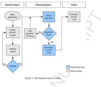
2. Development Process
The development process is shown in Fig. 1 and accommodates two development roles and one testing role. A domain expert defines the application state space and specifies the application policy. Domain experts are not required to be proficient in the field of planning and optimisation. A planning expert adds new planning and optimisation algorithms to the library and defines mappings from our planning model API to algorithm logic. The planning expert can add algorithms without reference to pervasive computing middleware services or sensor and actuator placement. A tester evaluates the performance of the generated code.
Create domain model
Validate
Domain Expert Planning Expert Tester
New application
Specify policy
Select algorithm
Algorithm found
Generate control
units Add
algorithm to library
Pass Fail
Yes No
Evaluate control
units
[image:4.595.151.475.90.369.2]Automated step Manual step
Figure 1: Development process roles.
1. The domain expert constructs a domain model using XML schemas provided.
2. The domain expert writes a policy file specifying the desired behaviour of the application.
3. The first transformation algorithm is then used to validate the domain model and policy, and if they are valid, to populate a planning model for the application.
4. The next step is to choose an appropriate planning or optimisation algorithm. A planning expert can manually specify with algorithm they wish to use or they can allow the second transformation to automatically select one. Once the algorithm is selected manually or automatically, the second transformation will generate planning or optimisation control units for the application.
The planning expert may wish to evaluate the performance of a selected algorithm. Many planning and optimisa-tion algorithms have parameters that can be tuned or customised for each applicaoptimisa-tion domain. Parameter values can be specified at layer 4 of the domain model. An evaluation platform is also provided to facilitate testing the performance of control units.
2.1. Tool Support
The following tool support is provided to enable the development process:
• A suite of domain model and policy XSD schemas.
• A validation engine to check the validity of domain models. The LXML parser is used to validate and parse XML documents1.
• A transformation engine to parse a domain model and populate a planning model that provides an API for use by planning and optimisation algorithms. The first transformation algorithm provides support for validating the domain model and policy and for transforming the domain model to a planning model.
• A transformation engine to choose a suitable algorithm and generate application code. Both transformations are written in Python. The second transformation algorithm provides support for validating the planning model and algorithm taxonomy and for generating control units for the application.
• A library of planning and optimisation algorithms implemented in Python.
• An evaluation platform used by a tester to evaluate the performance of generated application code. This platform provides simulated sensor data and run-time middleware services for sensor and actuator discovery and access. The planning expert adds new planning and optimisation algorithm implementations to the library and updates the algorithm taxonomy to specify the problem type and set of environmental conditions in which the algorithm is suitable for use. When an algorithm is added to the taxonomy a function is defined by the planning expert to map algorithm logic onto planning model components. This is a one-time effort and once the mapping has been specified,
the algorithm can be repeatedly applied to new matching problem instances. The mapping logic varies with the algorithm type. Planning model components provide an API to planning experts that abstracts away from sensor and actuator placement and quality to expose run-time application state values as discrete and continuous likelihood functions. Planning model components also provide access to reward model and state-transition information, defined by the domain expert using the domain-model specifications.
The use of sensor and actuator infrastructure requires that the control units make use of a middleware for access and query operations. The control units operate by providing information for sensor/actuator selection and identification
and assume middleware abstractions for discovery and lookup services. Such abstractions are provided by a range of pervasive computing middlewares such as [5] [6] [7] and are not directly addressed in this paper.
2.1.1. Evaluation Platform
The evaluation platform provides the following components:
• Sensor and Actuator Simulator. A lightweight simulator is provided to generate sensor and actuator data for use in the evaluation scenarios. Sensor and actuator data can be simulated from specified discrete and continuous probability distributions.
• Middleware services. The middleware service is built around the lightweight Python Pyro Distributed Object system [8]. State-variable objects can be deployed, registered with middleware lookup services, and invoked by planning and optimisation algorithms and other state-variable objects. The middleware also supports sensor lookup and discovery services invoked at runtime using spatial queries generated by the domain and planning model transformations.
• Spatial Query Support. Spatial queries are derived from topology abstractions and domain model spatial at-tributes and allow the automation of sensor and actuator, and state-variable object discovery and lookup. Spatial query execution is provided by the PostgreSQL engine with PostGIS support for geographic objects using the SFS standard.
• Inference Engine. State-variable objects provide support for competitive and feature/decision level state
infer-ence techniques. The libraries used in competitive fusion were developed as part of the tool chain. The Hugin Inference Engine [9] is used to provide the required support, however Hugin exposes an API in C/C++and Java
[10], therefore we implemented a python interface to the Hugin inference engine using the SWIG interface tool [11].
3. Domain Model Specification
3.1. Domain Model Topology Abstraction
The domain model design uses a topological abstraction to allow pervasive computing applications to be pro-grammed independently of the runtime conditions. A topological approach is adopted to model the spatial relation-ships of sensors, actuators, policies, and states as geometric shapes defined by sequences of coordinates based on a chosen, well-known coordinate system. The shapes may be chosen to reflect the physical space occupied by objects or may describe the sensing zone of sensors or the physical region in which a policy is to be deployed.
Applications using spatial attributes can exploit implicit relations between spatial attributes to link diverse infor-mation together for an application-specific purpose, without the need to specify explicit interaction between objects [12]. They may access spatially-related information, for example, by means of exploiting the distance between shapes or by exploiting containment and intersection relations. This might, for example, enable a vehicle-based information system to retrieve the locations of car parking facilities within a certain distance from its current location.
Topological abstractions make use of the spatial attributes of domain-model elements to simplify the design and implementation of planning and optimisation algorithms. They are used by the transformations to generate code to automatically invoke middleware services used in sensor and actuator discovery and lookup, and to identify the application deployment region.
3.2. Evaluation Scenarios
To help clarify the presentation of the domain model and transformations, we introduce two scenarios in which our development process is applied. In the first scenario an optimisation algorithm is used to optimise the use of CCTV camera infrastructure in a city and in the second scenario a planning algorithm is used to control the operation of traffic junction signal controllers in a city.
3.2.1. CCTV Selection Scenario
We assume that the city contains hundreds of CCTV sensors placed at various traffic junctions and that council
staffon duty monitor and detect traffic accidents and congestion using 30 screens that can be used to display CCTV
image streams. The desired behaviour is to select the 30 mostinterestingCCTV data streams to display from the hundreds of available cameras. The criteria by which a CCTV camera is considered interesting, are defined by the domain expert to be a function of weather, traffic demand and pedestrian presence. There is a further requirement that
the set of useful CCTV cameras should be chosen to also provide the maximal geographic spread or coverage over the city transport network. This application therefore requires a bi-criteria optimisation algorithm to be deployed in a pervasive computing environment and the use of state inference techniques to infer application states from sensor data.
3.2.2. Junction Controller Scenario
We assume the council wish to manage the behaviour of all traffic-light controllers in the following manner. Each
traffic light controller should access and use any available sensor data to measure the traffic demand and to detect
the presence of emergency vehicles. When the presence of an emergency vehicle is detected at a traffic junction, a
traffic light phase should be chosen to accommodate that vehicle’s transit through the junction. In the absence of an
emergency vehicle being present the system should, at the end of each phase, switch to the phase that has the highest traffic demand at that time. This application therefore requires a decision making algorithm, robust to uncertain
application state, to be deployed at multiple locations in a pervasive computing environment.
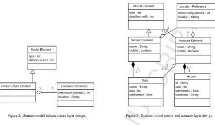
3.3. Layer 1
Model Element
type : int dataSourceID : int
Infrastructure Element Location Reference
referenceSystemID : int location : String
[image:7.595.295.505.90.350.2]1 1
Figure 2: Domain model infrastructure layer design.
Model Element
type : int dataSourceID : int
Actuator Element
name : String mobile : boolean Sensor Element
name : String mobile : boolean
Location Reference
referenceSystemID : int location : String
Data
name : String cost : int confidence : float
Action
id : String cost : int confidence : float transition : String 1
1..* 1
1..* 1
0..1
1 1 1
1
Figure 3: Domain model sensor and actuator layer design.
Both scenarios share a common layer 1 that specifies the city’s static road network infrastructure specified as a series of signalised junctions connected by road links that allow traffic to flow from one junction to another. A
standard model is used to represent the road network based on the Paramics traffic simulator2, formatted using the
SFS spatial data standard and stored in a PostgreSQL GIS database. There are 247 junction elements whose spatial attributes are represented as circles of radius 20 metres from junction centre points and 2800 road link elements whose spatial attributes are represented as multi-polygon geometries summing the geometries of road links. Layer 1 data was obtained from a Paramics model of Dublin city.
3.4. Layer 2
Layer 2 specifications are used to model the sensor and actuator infrastructure in the deployment environment. The data provided by sensor and actuator elements modelled at layer 2 are typically not available until runtime and are assumed to be accessed at runtime through a pervasive computing middleware service. The design of this layer is shown in Fig. 3. Sensor and Actuator classes inherit from a base Model Element class and both have an associated spatial attribute. Layer 2 sensor objects contain one or more data objects used to specify what kind of values the sensor provides, and an actuator object contains zero or more data objects and one or more action objects used to specify what actions an actuator supports. Data and action objects are used at runtime when interpreting sensor and actuator data. Data objects have a confidence attribute indicating the degree of confidence associated with individual sensor readings. For discrete sensor data the confidence measure is a probability value between 0 and 1 indicating the likelihood of sensor data being correct. For continuous sensor data the confidence value is the variance associated with sensor readings. Determining the confidence value for a particular sensor will require either the use of self-describing sensors [14], or else may be obtained from sensor specifications and manufacturer documentation. Data and action objects have a cost attribute which may be used to specify power or communication charges involved in accessing sensors and actuators.
Actuators implement actions that may effect a change in the state of a system. The spatial attribute of an actuator
includes its location and the region of the environment over which its actions have an effect. Action objects have a
confidence attribute which is a probability assigned to a successful state transition caused by the actuator.
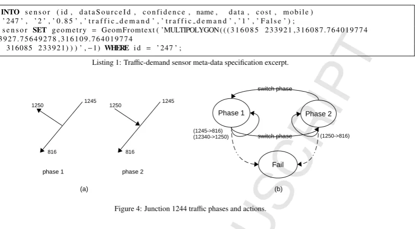
[image:7.595.68.512.92.351.2]INSERT INTO s e n s o r ( id , d a t a S o u r c e I d , c o n f i d e n c e , name , d a t a , c o s t , m o b i l e )
VALUES( ’ 247 ’ , ’ 2 ’ , ’ 0 . 8 5 ’ , ’ t r a f f i c d e m a n d ’ , ’ t r a f f i c d e m a n d ’ , ’ 1 ’ , ’ F a l s e ’ ) ;
UPDATE s e n s o r SET g eo m et r y = GeomFromtext ( ’MULTIPOLYGON( ( ( 3 1 6 0 8 5 233921 ,316087.764019774
2 3 3 9 2 7 . 7 5 6 4 9 2 7 8 , 3 1 6 1 0 9 . 7 6 4 0 1 9 7 7 4
. . . 316085 233921) ) ) ’ ,−1) WHERE i d = ’ 247 ’ ;
Listing 1: Traffic-demand sensor meta-data specification excerpt.
[image:8.595.94.520.92.327.2]
Figure 4: Junction 1244 traffic phases and actions.
The effects of actions are specified using state charts. The domain model implementation uses a modified version
of the State Chart XML (SCXML) language, which specifies state transition information based on Harel State Tables and which supports composite state spaces and probabilistic transitions [15], thus making it suitable for specifying state charts for pervasive computing environments.
Layer 2 of the CCTV Selection scenario domain model contains three sensor elements and one actuator element. An inductive loop sensor [16] provides sensor data on traffic demand and travel times. Weather station sensors are
modelled to provide data on rain fall levels at each junction. We also assume that a stationary pedestrian presence sen-sor is present at each junction to provide data on pedestrian levels. The spatial attribute of the weather and pedestrian sensors is specified as an ellipse representing their sensing areas.
Listing 1 shows a traffic demand sensor entry in the domain model. The sensor has a confidence measure of 0.85
which is interpreted as the likelihoodP(tra f f ic demand==high|S ensorReading==high)=0.85. A cost of 1 unit is associated with obtaining each sensor reading and the mobility flag is set to false. The spatial attribute of this sensor is specified as a multi-polygon shape, using an SFS function to convert a string of coordinates specified in the Irish National Grid reference system, into a spatial geometry. Spatial data on fixed infrastructure is often available from local authorities and through initiatives such as OpenStreetMap3which distribute spatial data freely.
Layer 2 for the Junction Controller scenario contains inductive loop sensors, emergency vehicle detection sensors, and traffic controller actuators located at each junction and responsible for switching traffic phases. The actions
specified for each junction controller consists of the available traffic-control phases at that junction. An example of
the set of actions available at Junction 1244 is shown in Fig 4(b). The actuator specification for Junction 1244 is shown in Listing 2. From Listing 2 actuator 1244 has a name which is the junction number and a mobility flag which is set to false and provides two actions: phase 1 and phase 2. Following SCXML terminology, these actions are described using state attributes. Each state attribute contains the following information:
• an id, which is the action name.
• the geometry or region over which the action is executed.
• each datamodel element contains a cost and confidence element indicating the cost of invoking this action on the actuator and the likelihood of the action invocation succeeding.
<a c t u a t o r>
<name>1244</name>
<m o b i l e>f a l s e</m o b i l e>
<s t a t e>
<i d>p h a s e 1</i d>
<g eo m et r y>MULTIPOLYGON( ( ( 3 1 6 2 8 0 233765316287019124818 233762994535766316265019124818
233685994535766316258 233688316280 233765) ) )</g eo m et r y>
<d a t a m o d e l>
<c o s t>1</c o s t>
<c o n f i d e n c e>0 . 9 9 5</c o n f i d e n c e>
<!−− l i n k 1245−816 −−> <!−− l i n k 1245−1250 −−>
</d a t a m o d e l>
<t r a n s i t i o n e v e n t = ” s w i t c h−p h a s e 2 ” cond = ” r a n d l e s s e q 0 . 9 9 5 ” t a r g e t = ” p h a s e 2 ”/>
<t r a n s i t i o n e v e n t = ” s w i t c h−f a i l ” cond = ” r a n d g t 0 . 9 9 5 ” t a r g e t = ” f a i l ”/>
</s t a t e>
. . . .
Listing 2: Excerpt of actuator specification for junction controller 1244.
• one or more transition elements indicating the state-action combinations to which the actuator can transition and the likelihood of the transition succeeding.
An actuator record should be created to match every instance of a junction controller in the city.
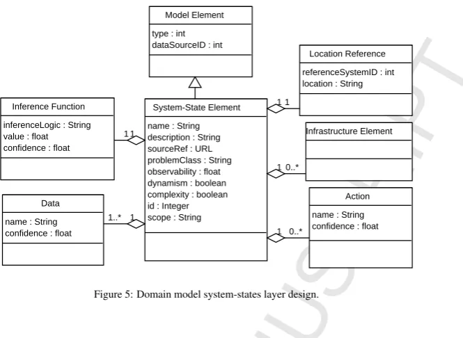
3.5. Layer 3
Layer 3 of the domain model is used to specify the state-space of a pervasive computing application. Determining state values typically requires access to sensors and actuators distributed throughout the environment, the quality and spread of which will often be unknown at design time. Layer 3 system-state elements are used by domain experts to specify the logic for calculating the values of application states, independently of run-time conditions. System-state elements are composed using layer 1 and 2 elements to specify the types of sensor data and actuator actions, and the types of infrastructure in the deployment environment, that are required to calculate run-time values for the application state space. Examples of system-states include vehicle throughput at a traffic junction, journey time along a road link
and power consumption in a room.
The design of this layer is shown in Fig. 5. Each system-state has a scope that indicates the region of the deploy-ment environdeploy-ment over which it is defined. Layer 1 and 2 eledeploy-ments referenced in a system-state definition are mapped at runtime onto matching physical entities in the region of the deployment environment described by the scope.
A system-state specification includes an inference function whose logic is used to calculate state values from the run-time values of sensor data and actuator actions. Sensor and actuator meta-data are used in the inference function to quantify the uncertainty associated with state values. Uncertainty is specified using discrete and continuous likelihood functions for the true value of the system-state given the available sensor data.
System-state elements have a problemClass attribute indicating that the element belongs to either a planning or op-timisation problem. Deployment environment conditions are specified using dynamism, complexity, and observability attributes that are used to indicate respectively: that the state’s value can be affected by uncontrolled state-transition
events; that it may be computationally difficult to compute the value of a system-state; and that the application state
space values are expressed as probabilities rather than direct observations. In the event that the domain expert does not specify which planning or optimisation algorithm to use, the transformations will use these four attributes to select an appropriate planning or optimisation algorithm for the problem.
Layer 3 for the CCTV Selection scenario contains specifications of three system-states: JunctionInterest, Max-imalDistance, and DegreeofInterest. A JunctionInterest system-state is specified to be a monotonically increasing function of worsening weather conditions, pedestrian presence, and increasing traffic demand. Domain experts specify
Model Element
type : int dataSourceID : int
System-State Element
name : String description : String sourceRef : URL problemClass : String observability : float dynamism : boolean complexity : boolean id : Integer scope : String Data
name : String confidence : float
Action
name : String confidence : float Infrastructure Element
Location Reference
referenceSystemID : int location : String
1 1..*
1 0..* 1 0..* 1 1 Inference Function
inferenceLogic : String value : float confidence : float
[image:10.595.141.474.94.337.2]1 1
Figure 5: Domain model system-states layer design.
that a value for this system-state is to be calculated at each instance of a junction infrastructure element contained in the scenario domain model. The implementation attribute contains a reference to an inference function that uses a Bayesian network to combine the inputs to produce an output value for the system-state.
Figure 6: Bayesian network structure for JunctionInterest.
Rain
Mean 0.0 Variance 0.25
Traffic Volume
Low 0.2 Medium 0.4 High 0.4
Junction Interest
Pedestrians False True Traffic Volume Low Medium High Low Medium High Mean 1 3 5 3 5 7 Surface Water 5 5 5 5 5 5 Variance 2 2 2 2 2 2
Surface Water
[image:10.595.69.520.381.549.2]Mean 0.0 Rain 1.2 Variance 0.25
Figure 7: Bayesian network conditional probabilities for Junction-Interest.
Fig. 7 shows the conditional probability tables specified by the domain expert in the inference function. The hybrid Bayesian network contains a discrete Boolean Pedestrian node indicating whether pedestrians are present or not and a discrete TrafficVolume node taking the values: “high”; “medium” and “low”. It also contains continuous
SurfaceWa-ter, Rain and JunctionInterest nodes. A sample conditional probability from Fig. 7 readsP(S ur f aceWater|Rain)= N(1.2×Rain,0.25), i.e., the continuous variable SurfaceWater has a mean value that is 20% higher than the values reported by the Rain sensor and a constant variance of 0.25. Such a specification might reflect the belief of the domain expert that the rain sensors in general underestimate the amount of surface water by 20%.
<s y s t e m S t a t e> <i d>001</i d>
<name>J u n c t i o n I n t e r e s t</name>
<d e s c r i p t i o n>T h i s s t a t e m e a s u r e s t h e d e g r e e o f i n t e r e s t o f a s i n g l e J u n c t i o n</d e s c r i p t i o n>
<p r o p e r t i e s>
<c o m p l e x i t y>f a l s e</c o m p l e x i t y> <dynamism>t r u e</dynamism>
<o b s e r v a b i l i t y>p a r t i a l</o b s e r v a b i l i t y>
</p r o p e r t i e s>
<s c o p e>
<t y p e>e l e m e n t</t y p e> <v a l u e>j u n c t i o n</v a l u e>
</s c o p e>
<i n p u t s>
<l a y e r 1>
<name>i d</name> <name>g eo m et r y</name>
</l a y e r 1>
<l a y e r 2>
<name>r a i n</name>
<name>p e d e s t r i a n s</name>
<name>t r a f f i c v o l u m e</name>
</l a y e r 2>
</i n p u t s>
<!−− I m p l e m e n t a t i o n s −−>
<i m p l e m e n t a t i o n>
<s o u r c e R e f>J u n c t i o n I n t e r e s t</s o u r c e R e f>
</i m p l e m e n t a t i o n>
</s y s t e m S t a t e>
Listing 3: JunctionInterest system-state specification.
A DegreeofInterest system-state is defined to sum the JunctionInterest value for each junction in the candidate set of CCTV cameras associated with the junctions. This system-state is included so that the scenario policy can be easily specified as a function of candidate sets of CCTV cameras.
Layer 3 of the Junction Controller scenario contains two system-states. A TrafficDemand system-state can take
the values:“low”; “medium”; and “high”. An EmergencyVehiclePresent system-state that can take values: “true” or “false”. These system-states are associated with traffic phase actuator elements in layer 2 of the domain model and
have a scope equal to the spatial attributes of phase elements. Both system-states are dynamic in that their values can fluctuate independently of the action taken by the traffic light. Likewise both system-states are partially observable as
their values are inferred from sensor data. The complexity attribute is set to false for each system-state.
3.6. Layer 4
Layer 4 holds domain-specific knowledge such as the algorithm type to be used and values for free parameters of the algorithm. Layer 4 is provided to allow the domain or planning expert to customise the performance of the planning and optimisation algorithms that will be embedded in the generated control units. Information specified at this layer is algorithm specific and can include data such as prior probabilities on the values of system-states and energy levels and cooling schedules for stochastic search algorithms. In the absence of layer 4 data the transformations will select an algorithm from the library and use default values for its free parameters.
Layer 4 of the Junction Controller scenario contains prior probability mass functions (0.4,0.4,0.2) and (0.1,0.9). for the TrafficDemand and EmergencyVehiclePresent system-states respectively, indicating that traffic demand will
<p o l i c y>
<s c o p e>g l o b a l</s c o p e>
<problem>o p t i m i s a t i o n</problem>
<s t a t e>
<name>M a x i m a l D i s t a n c e</name> <r e w a r d>
<t y p e>c o n t i n u o u s</t y p e>
<v a l u e>maximise</v a l u e>
<w e i g h t>1</w e i g h t>
</r e w a r d>
</s t a t e>
. . . .
Listing 4: Policy excerpt from the CCTV selection scenario.
<p o l i c y>
<s c o p e>g l o b a l</s c o p e>
<problem>p l a n n i n g</problem>
<s u b t y p e>s i n g l e d e c i s i o n</s u b t y p e>
<s t a t e>
<name>T r a f f i c D e m a n d</name> <r e w a r d>
<t y p e>d i s c r e t e</t y p e>
<r a n g e>heavy−medium−l i g h t</r a n g e>
<a c t i o n>s w i t c h−p h a s e</a c t i o n>
<v a l u e>10−5−1</v a l u e> <w e i g h t>1</w e i g h t>
</r e w a r d>
</s t a t e>
. . . .
Listing 5: Policy excerpt from the junction controller scenario.
4. Policy Specification
Policy specification provides a high-level method for the domain expert to control application behaviour. Appli-cation policy is specified by associating rewards with the range of possible system-state values and/or state-action
combinations. The transformation algorithms use the policy specification to create a reward model attached to states and/or actions. An XML schema is provided to allow validation of the policy specification and contains the following
information:
• A scope attribute identifies the region of the physical environment over which the application is to be deployed.
• A problem attribute indicates whether the problem is a planning or optimisation problem and influences the selection of planning model components. An optional subtype element can be used to indicate whether or not the problem is a single or sequential decision problem and is used as an aid to algorithm selection.
• A state attribute identifies system-states over which the policy is defined.
• Each state attribute contains a mandatory reward sub-attribute. Reward elements contain a number of attributes: a type attribute identifying whether the system-state produces data values that are discrete or continuous; a range attribute specifies a hyphenated list of values that discrete state values can take, e.g., “high”, “medium” or “low” and their corresponding reward values. For continuous data the value can be specified as “maximise” or “minimise”. A weight attribute can be used to prioritise competing system-states. An action is an optional attribute used to associate an action with the state and reward.
An excerpt of the policy specification for the scenarios is shown in Listings 4 and 5. The CCTV Selection scenario policy specifies the application scope to be of value “global” indicating that planning model components will be generated by matching all system-state scopes against elements throughout the geographic region covered by the domain model. A reward attribute for each system-state specifies that the system-states referenced in the policy are continuous valued, of equal weight and that the optimisation algorithm should attempt to maximise the value of each system-state.
The Junction Controller scenario policy specifies the application scope to be of value “global”. The TrafficDemand
system-state can take values: “high”, “medium” and “low” with associated rewards 10, 5, 1. An action attribute is used to associate a ”switch-phase” action with each reward. The value attribute provides a numeric value for each corresponding value of the system-state.
As an indication of the domain modelling effort required for the CCTV Selection scenario, the combined layer
5. Model Transformations
The model transformations produce application code that executes over an assumed middleware to provide the desired planning and optimisation behaviour as expressed in the domain model and policy. The first transformation extracts information from the domain model to populate planning model components that provide a programming interface to pervasive computing environments modelled on a five-tupleP=(S,A,T,O,R) where:
• S ={s1,s2, ..}is the set of system states;
• A={a1,a2, ..}is the set of actions provided by actuator functionality; • T(s,a,s0
) represents a stochastic state-transition function that gives the probabilityP(s0
|s,a) of moving to state
s0
if the actionais performed in states.
• O = {o1,o2, ..} is the set of observations that are produced by the sensor infrastructure in the region. An
observation or sensor model function O(s0
,a,o) gives the probability P(o|a,s0
) of observingo if actiona is performed and the resulting state iss0
.
• R(s,a,s0
) represents the immediate reward for performing actionawhile in statesand moving to states0 . Application state is represented as variables that provide estimates of changing value and certainty at runtime. From P, each si ∈ S represents a system-state element that is implemented by a set of state-variable objects.
State-variable objects are planning model components, generated by the transformations using domain model system-state specifications, to perform sensor fusion and system-state inference services. They perform the sensor model function
O(s0
,a,o), by combining spatial attributes with named layer 2 sensor data and actuator action inputs, to invoke mid-dleware services and return the run-time values of system-states in the deployment environment. The number of state-variable objects required for each system-state is calculated using the system-state and policy scope information. For example, if a system-state has a scope of type “element”, a state-variable object is created for each matching element within the policy scope.
Actuator objects are generated from layer 2 elements to provide an interface to actions and associated state-transitions currently specified in SCXML. Support for additional state-transition formats such as dynamic Bayesian networks (DBNs) could be added by extending the domain model transformation to compile the DBN format into the internal representation for state-transition systems used in the planning model.
Reward model entriesR(s,a,s0
) are implemented as a multi-dimensional hash-table containing tables indexed by each system-state name in the domain model. For discrete states, numeric rewards are stored for state/action
combi-nations extracted from the policy specified by the domain expert. Continuous states are indexed with maximisation or minimisation tag values.
5.1. Domain Model To Planning Model Transformation
The logic of this first transformation is summarised under the following three headings:
1. Parse the policy and system-state specifications.
The policy file and system-state specifications are validated using their respective schemas. The policy scope indicates the extent of the region over which the application is to be deployed. The problem type will be either planning or optimisation and determines the required planning model components. The scope, complexity, dynamism and observability properties are recorded for each system-state. The set of layer 1, 2 and 3 inputs are read for each system-state and a reference to the state inference function is recorded.
2. Planning problems.
3. Optimisation problems.
For complex optimisation problems the state space will often be too large to evaluate fully and the overhead of creating a full set of state-variable objects is impractical. For example, in the CCTV Selection scenario, there are 247!
(247−30)! permutations of 30 CCTV installations that can be chosen from the 247 available.
Heuris-tic optimisation algorithms manage complexity by exploring random subsets of an application state space. To accommodate random exploration of complex pervasive computing state-spaces, the domain-model transfor-mation creates state-generator factories used by optimisation algorithms to produce state-variable objects with randomly chosen spatial attributes on demand at runtime. State-variable objects generated for optimisation problems are functionally identical to those used in planning problems.
5.2. Planning Model Sensor Fusion Support
State-variable objects combine their spatial attributes with layer 2 input names and perform sensor and actuator lookup and access operations by invoking middleware services. By default state-variable objects perform low-level automated competitive fusion of sensor data. Competitive sensor fusion techniques are employed when multiple sensors deliver independent measures of the same property and use weighted average algorithms to reduce the effects
of uncertain and erroneous measurements [17].
If multiple sensor readings for a layer 2 input are returned to a state-variable object following its middleware request, they are automatically combined in a fused likelihood function calculated as the product of the individual probability mass or density functions of each sensor reading. State-variables implement this as follows for discrete and continuous sensor data. Assume that a set of N independent sensor readings{y1,y2, . . .yn}relating to the true value
of a layer 2 inputΘis obtained from sensor infrastructure at timet. It is assumed that they come from a common
(perhaps unknown) distribution and are independent observations of the same value. The sensor model from layer 2 of the domain model provides a conditional probabilityP(yi|Θ) i.e., the likelihood of the value of the layer 2 input
given the sensor data observed. For discrete sensor readings the conditional probabilities are combined as:
P(y1|θ)×P(y2|θ). . .P(yn|θ)= N Y
i=1
P(yi|θ) (1)
The same approach is used to automatically fuse continuous sensor readings. The layer 2 sensor model provides a con-ditional probability for normally distributed scalar valued continuous sensor readings specified using the parameters
{µ, σ}obtained respectively from the sensor reading and sensor confidence attribute, and combined as:
ˆ µ=
P iyi/σ2i P
i1/σ2i
and σˆ = Pn 1 i=1(1/σ2i)
(2) Eqn. 2 provides the parameters of a fused likelihood function calculated fromNpieces of sensor data. Under the assumption of normally distributed errors this is also the maximum likelihood estimate, the weighted least squares estimate, and the linear estimate whose variance is less than that of any other linear unbiased estimate [18].
High-level inference functions defined by the domain expert in layer 3 system-state elements are also executed by state-variable objects at run-time. The fused likelihood values calculated for each layer 2 input are combined by the state inference function specified by the domain expert, to return a value for the system-state to the planning or optimisation algorithm. Figs. 6 and 7 show a Bayesian network defined to provide the high-level state inference logic to measure JunctionInterest values at all 247 traffic junctions in the CCTV Selection scenario. At runtime, optimisation
algorithms invoke state-variable objects to return a current JunctionInterest value. The state-variable object initially issues middleware sensor discovery queries and access requests within the deployment region associated with their spatial attribute. They then update each node of the Bayesian network corresponding to a layer 2 input, with fused likelihood functions described above. The Bayesian network instances are then executed and the posterior value of the JunctionInterest state for each junction is returned to the optimisation algorithm.
environment with a proliferation of sensors and other regions with few or no sensors. A region with many sensors providing data for the same state input should have a lower uncertainty than a region with less sensor data. Automated competitive fusion allows varying levels of sensor coverage to be exploited by planning and optimisation algorithms at runtime.
5.3. Planning Model To Control Unit Transformation
The logic of this second transformation is summarised under the following two headings:
1. Read algorithm selection logic and problem type.
The algorithm library is validated using the library XSD schema. Information indexing the available algorithms by problem type and environment properties is read from the algorithm taxonomy. The problem, complexity, observability, and dynamism attributes are read for each system-state contained in the planning model. 2. Algorithm selection and control unit instantiation.
The problem and subtype attributes in system-state templates are used to identify the root branch of the algo-rithm taxonomy and the domain characteristics are used to select a particular algoalgo-rithm. The algoalgo-rithm compo-nents are then mapped to the planning model compocompo-nents and control units are instantiated using the templates shown in Algs. 1 and 2. Algorithms selected automatically are assigned default values for free parameters, specified by the planning expert when the algorithm is added to the library.
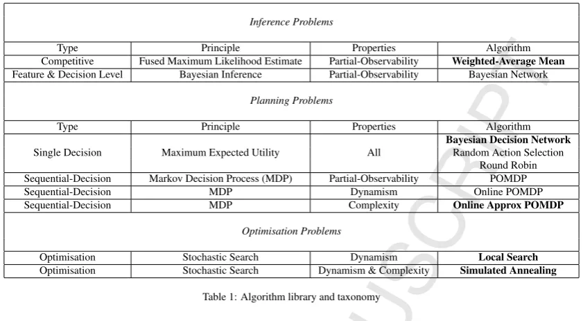
5.3.1. Algorithm Selection
Table 1 lists the library of algorithms we provide for inference, planning, and optimisation problems. The first column of each section lists the problem type. The second column shows the type of algorithm and the third column lists the system-state properties deemed relevant to selecting an algorithm. The fourth column lists the algorithms provided for a combination of problem and system-state properties.
The planning expert can implement multiple algorithms for each problem type and property set and can specify which algorithm to use in the domain model. However if automatic algorithm selection is used then only algorithms referenced in the taxonomy are considered for selection. The algorithms available for automatic selection are shown in bold print in Table 1.
The taxonomy specifies that competitive inference problems are implemented with a weighted average mean algo-rithm in partially observable environments. Feature/decision-level state inference problems are currently implemented
using a Bayesian network library that has been integrated into the algorithm library.
Domain experts may not be familiar with Bayesian networks and may choose to use another high-level inference technique. The planning model interface exposes state values as likelihood functions to planning and optimisation algorithms. Additional state inference techniques providing likelihood functions for application state can be added to the library without impacting the planning and optimisation algorithms contained in the algorithm library.
Single decision problems are modelled using the principle of maximum expected utility and implemented us-ing Bayesian decision networks. Sequential decision plannus-ing problems are implemented usus-ing a Markov Decision Process (MDP) framework [2]. If the environment is partially observable and dynamic, then an online approximate POMDP algorithm is chosen. The POMDP framework supports a wide range of exact and approximate, online and offline approaches to planning [19]. Solutions to optimisation problems are based on heuristic algorithms. If the
environment is dynamic a stochastic approximation algorithm is chosen. For applications with complex state spaces, a simulated annealing algorithm is chosen. The association of problem type to algorithm selection is informed by reference to the literature and can be amended by editing the taxonomy.
5.3.2. Control Unit Templates
Inference Problems
Type Principle Properties Algorithm
Competitive Fused Maximum Likelihood Estimate Partial-Observability Weighted-Average Mean
Feature & Decision Level Bayesian Inference Partial-Observability Bayesian Network
Planning Problems
Type Principle Properties Algorithm
Single Decision Maximum Expected Utility All Bayesian Decision NetworkRandom Action Selection
Round Robin
Sequential-Decision Markov Decision Process (MDP) Partial-Observability POMDP
Sequential-Decision MDP Dynamism Online POMDP
Sequential-Decision MDP Complexity Online Approx POMDP
Optimisation Problems
Optimisation Stochastic Search Dynamism Local Search
[image:16.595.79.500.94.326.2]Optimisation Stochastic Search Dynamism & Complexity Simulated Annealing
Table 1: Algorithm library and taxonomy
returns the action that maximises the reward at each time step. For sequential planning problems the control unit selects an action that maximises the reward over a planning horizon.
Alg. 2 shows the execution cycle of a control unit for an optimisation problem. A collection of state-variable objects evaluated by an optimisation algorithm is referred to as a candidate solution. In line 1, a candidate solution θ, from the domain of possible solutionsΘ, is initially generated subject to the system-state specifications.
Heuris-tic optimisation algorithms generate initial candidate solutions stochasHeuris-tically. Lines 3-5, invoke the state inference functions provided by state-variable objects to obtain values for candidate solutions. In line 8, the control units use
L(θ), a loss function generated from the policy specified by the domain expert to evaluate the candidate. The logic governing candidate generation and evaluation is specific to the optimisation algorithm contained within the control unit. The stopping criterion tested in line 2 and the generation of new candidate solutions in line 10 are also specific to the optimisation algorithm contained within the control unit.
5.4. Scenario Transformations
The CCTV Selection scenario is specified in Listing 4 to be an optimisation problem. The domain-model trans-formation populates the planning model components to provide a state-generator factory and a reward model from the policy and system-state specifications At runtime, 30 state-variable objects associated with the JunctionInterest system-state query for sensor data, compute a fused likelihood function for each layer 2 input and then enter the likelihood data into the Bayesian network specified by the domain expert. The mean value returned by 30 Bayesian networks representing candidate sets of 30 junctions are summed by DegreeofInterest state-variable objects. The MaximalDistance state-variable objects calculate the geographic spread of the candidate set of 30 junctions.
The algorithm taxonomy currently specifies that a simulated annealing algorithm based on the SMOSA algorithm [20] is preferred for optimisation problems with complex, partially-observable and dynamic state spaces. The SMOSA algorithm supports multi-objective problems and generates solutions that are optimal in the sense that no other solu-tions in the search space are superior to each other when the two objectives are considered. Such solusolu-tions are known as Pareto-optimal [20].
In line 1 of Alg 2, a candidate solution setθof 30 CCTV cameras, from the 247!
(247−30)!possible solutions is generated.
In lines 2-5, sensor data and inference functions are used to calculate DegreeofInterest and MaximalDistance values forθ. The SMOSA algorithm works by randomly selecting and evaluating a neighbours0
of the current states, and probabilistically accepting or rejectings0
Algorithm 1: Planning problem control unit template.
Input:P: a planning model; Alg: an instance
of a planning algorithm.
foreachsi∈S do
1
integrate sensor evidence intosi; 2
calculateP0 (si); 3
end
4
foreachaction ai∈Ado
5
calculateAlg(ai,s0i), the reward for taking 6
action A;
end
7
returnthe best action fromA;
8
Algorithm 2: Optimisation problem control
unit template.
Input:P: a planning model; Alg: an instance
of an optimisation algorithm. generate candidate set(s){S(θ)∈Θ}; 1
whilenot finisheddo
2
foreachθ∈S(θ)do
3
integrate sensor evidence intoθ;
4
calculateP0 (θ);
5
end
6
foreachθ∈S(θ)do
7
evaluate the loss functionL(θ) ;
8
end
9
generate new candidate set(s){S(θ)∈Θ}; 10
end
11
returnthe best solution fromS(θ);
12
to move to states of lower energy [20]. The number of evaluation iterations performed by the SMOSA algorithm is controlled through a run-count parameter.
The utility of solutions found by the SMOSA algorithm are dynamic due to fluctuating traffic volumes, weather
changes and pedestrian presence. The control unit should be re-run periodically to generate solutions in a dynamic environment. The planning expert can use layer 4 of the domain model to specify a range of possible values for the temperature and run-count parameters. Our tool-chain can be used by planning experts to empirically assess appropriate algorithms and parameters for applications.
The Junction Controller scenario is specified in Listing 5 to be a single-decision planning problem and the al-gorithm taxonomy specifies that Bayesian decision networks are used to implement control units for this class of problem. Decision networks are an extension of Bayesian networks to incorporate actions and utilities and provide a compact model for single-decision processes [21]. Given a stochastic transition function and some sensor evidence
E, actions are selected to maximise the expected utility (MEU), calculated as [22]:
EU(a|E)=X s0
P(s,a,s0,|e)U(s0) (3)
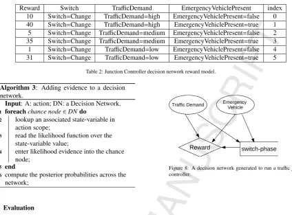
The planning-model transformation instantiates a template decision network at each junction controller actuator. The transformation algorithm obtains the decision network structure as follows: initially a chance (oval) node is created for each system-state template object which can be discrete or continuous depending on the system-state data type, subsequently decision nodes (rectangle) are created for actions supported by the actuator functionality, and finally a utility node (diamond) is created and configured with reward model data combined using an additive utility function and shown in in Table 2. The structure of the decision networks generated by the planning-model transformation for the Junction Controller scenario control units is shown in Fig. 8. The transformation algorithm then searches layer 4 data to find prior probabilities specified by the domain expert for system-states related to chance nodes.
Reward Switch TrafficDemand EmergencyVehiclePresent index
10 Switch=Change TrafficDemand=high EmergencyVehiclePresent=false 0
40 Switch=Change TrafficDemand=high EmergencyVehiclePresent=true 1
5 Switch=Change TrafficDemand=medium EmergencyVehiclePresent=false 2
35 Switch=Change TrafficDemand=medium EmergencyVehiclePresent=true 3
1 Switch=Change TrafficDemand=low EmergencyVehiclePresent=false 4
[image:18.595.70.495.90.403.2]31 Switch=Change TrafficDemand=low EmergencyVehiclePresent=true 5 Table 2: Junction Controller decision network reward model.
Algorithm 3: Adding evidence to a decision
network.
Input: A: action; DN: a Decision Network.
foreachchance node∈DNdo
1
lookup an associated state-variable in
2
action scope;
read the likelihood function over the
3
state-variable value;
enter likelihood evidence into the chance
4
node;
end
5
compute the posterior probabilities across the
6
network;
Figure 8: A decision network generated to run a traffic junction
controller.
6. Evaluation
This paper presents a development process incorporating concepts from the domains of model-driven engineering and automated planning. We present an empirical evaluation of the impact of our tool chain on the effort of developing
the scenarios and a quantitative evaluation of the performance of the planning and optimisation algorithms generated by the automated-planning component for the scenarios. This section is structured as follows. The evaluation met-rics used for development effort and algorithm performance are introduced. These metrics are then applied to the
two evaluation scenarios. Finally we discuss the implications of our results for automating the use of planning and optimisation algorithms in pervasive computing applications.
6.1. Evaluation Metrics
The following approach was used to measure the impact of the development process on reducing the development effort for applying planning and optimisation algorithms in pervasive computing environments. The lines of code
(LOC) provided by the domain and planning expert for each scenario were recorded. The size of the spatial query set produced by the automated transformations was recorded and used as a proxy measure for the development effort
provided by the transformation engine. The scenarios were then extended by adding new requirements and the LOC metric measured for the extended domain and planning expert development (DM and PL respectively). The transfor-mations were re-run and the increase in size of the spatial query data produced recorded. The ratio of increased domain and planning development effort in LOC was then compared to the ratio of the increase in spatial query data generated.
This value is referred to as the “degree of automation” and calculated as:δ(DM+PL)/ δ(Planning Model S ize). We are interested in algorithm performance insofar as it can be used to judge the efficacy of our development
6.1.1. Algorithm performance in the CCTV Selection scenario
The taxonomy specifies that the SMOSA algorithm be used for complex, dynamic optimisation problems. To assess the appropriateness of this selection, the SMOSA results are compared to results from a baseline local search algorithm (SA) also applied to the scenario. Fig. 9 shows the Pareto front mapped by the SMOSA algorithm over 500 evaluation cycles and using a range of starting temperatures: 100, 500, 1000 and 5000. Each point on the graphs indicates the DegreeofInterest and MaximalDistance values of a set of 30 CCTV cameras. The only parameter that varies for each graph in Fig. 9 is the temperature parameter, responsible for controlling exploration rate. Varying the temperature parameter produces a visible shift in solution quality with the best value obtained at a temperature of 5000, while a starting temperature of 100 ultimately finds a longer Pareto landscape of solutions. Fig. 9 also shows a normalised maximum point calculated by weighting equally the sets of DegreeofInterest (DI) and MaximalDistance (MD) Pareto-optimal values as: max{DIi/Pni DI+MDi/Pni MD}. The normalised maximum calculation prevents
one criterion with large absolute values outweighing another criterion with smaller absolute values. Rows 2-4 of Table 3 show the best results obtained for this scenario using the SMOSA algorithm. Column 4 shows the normalised maximum values obtained for the optimisation criteria while column 5 shows a scalar normalised value calculated to enable a direct comparison between the results. The number of sensor invocations required to produce these results is shown in Column 6. The best result was obtained at a mean cost of 71,712 sensor invocations. However a very close value was obtained over 50 runs at a temperature of 500 using only 7118 sensor invocations. For this scenario, careful tuning can result in a 90% reduction in cost, as measured in sensor invocations, with only a slight degradation in algorithm performance.
Algorithm Run Count Temperature 2D Maximum Normalised Ranking µSensor Invocations
SMOSA 50 500 223.59 398.34 0.3462 7118
SMOSA 100 500 223.59 398.34 0.3462 14028
SMOSA 500 5000 221.04 416.91 0.3522 71712
Algorithm Run Count Temperature 2D Maximum Normalised Ranking µSensor Invocations
SA 50 NA 191.52 367.75 0.3080 7173
SA 100 NA 212.95 359.82 0.3213 14344
[image:19.595.73.504.327.428.2]SA 500 NA 211.01 373.99 0.3259 71218
Table 3: CCTV Selection scenario algorithm comparison
The performance of the baseline SA algorithm over 500 runs is shown in Fig. 10. The SA algorithm only maintains one solution during its operation and the concept of Pareto-optimality cannot be applied. SA operates by randomly generating a candidate solution and comparing the utility of the new candidate to the existing candidate using the specified policy values. The utility is calculated from summing the values of each criteria. If one criterion has large absolute values this will outweigh a number or criteria with smaller absolute values. Fig. 10 plots the values of the candidate solutions generated as the algorithm executes. The plot of the solutions is not smooth, rather it is jagged with consecutive solution fitness moving up and down randomly. The solution that maximise both values appears on the top-right of the graph. Figs. 9 and 10 are plotted using the same scales so that visual comparisons between run numbers are visually meaningful. The number of sensor invocations required to obtain these values is shown in Table 3. The sensor invocation overhead associated with the SA algorithm is similar to that associated with the SMOSA algorithm.
Column 5 of Table 3 shows a normalised ranking of the performance of the SMOSA and the SA algorithms. It shows that the SMOSA algorithm consistently outperforms the SA algorithm for all run counts. In fact the SMOSA algorithm for a run count of 50 with 7118 sensor invocations outperforms the SA algorithm with a run count of 500 and with 71218 sensor invocations. This shows that the choice of optimisation algorithm has a big impact on the quality of solution and the cost associated with obtaining that solution. It also vindicates, for this problem, the selection of the SMOSA algorithm over the SA algorithm for complex problems in the taxonomy.
6.1.2. Development effort in the CCTV Selection scenario
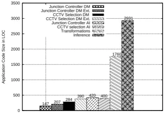
layer 3 system-states, EmergencyVehiclePresent and NumberEmergencyVehicles, were defined to detect and count the number of emergency service vehicles at junctions associated with selected sets of CCTV cameras. The addition of the system-states increase the domain model by 106 lines: 78 lines of XML and 28 lines of python. Of this increase, 10 lines of XML are for the policy extensions, 68 lines of XML are for the system-state definitions and the 28 lines of python code are for the inference functions.
Specifying the additional functionality increased the size of the domain modelling effort by c. 40% from 284
to 390 LOC. The SMOSA implementation and mapping was 400 LOC. However there was no additional planning development effort required as the SMOSA algorithm mapping logic is unchanged. The increase in development effort
δ(DM+PL) was 684/790 LOC=15%. The spatial query set generated by the transformation engine from the original
domain model was 69 KB in size. This increased to 118KB in size for the extended domain model. The degree of automation measure for the extended scenario was: 684/790 : 69/118, i.e., a 15% increase in development effort
was translated by the tool-chain into a 71% increase in application functionality as measured by the size of generated spatial query data. The increased functionality was mirrored in evaluation logs that show the original SMOSA control units performed 7118 sensor invocations over 50 runs while the extended SMOSA control units performed 8823 sensor invocations over 50 runs, an increase of c. 24%.
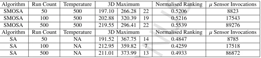
Algorithm Run Count Temperature 3D Maximum Normalised Ranking µSensor Invocations
SMOSA 50 500 197.10 266.28 22 0.5206 8823
SMOSA 100 500 202.88 320.39 19 0.5216 17543
SMOSA 500 500 219.55 296.41 22 0.5539 89276
Algorithm Run Count Temperature 3D Maximum Normalised Ranking µSensor Invocations
SA 50 NA 191.52 367.75 14 0.4847 8785
SA 100 NA 212.95 359.82 7 0.4259 17518
[image:20.595.68.516.280.380.2]SA 500 NA 211.01 373.99 13 0.4933 86872
Table 4: Extended CCTV Selection scenario algorithm comparison
Rows 2-4 of Table 4 show the optimal results obtained for the extended scenario using a temperature of 500 over 50, 100 and 500 runs. The best result (219.55, 296.41, 22) was obtained over 500 runs. Fig. 11 shows the behaviour of the SMOSA algorithm using this temperature and run count for the extended scenario. The best result normalised at 0.5539 and obtained at a mean cost of 89,276 sensor invocations is only 6% fitter than the 0.5206 result achieved after 50 runs at a mean cost of 8823 sensor invocations. The results obtained by the SA algorithm for 50, 100 and 500 runs in the extended scenario are shown in Rows 6-8 of Table 4 and show consistently poorer performance than SMOSA, highlighting again the importance of algorithm selection. A visual comparison between the SMOSA 3D plot and the SA 3D plot in Fig 12 reveals two interesting properties. Firstly, the surface of the 3D SMOSA plots are much smoother than the surface of the 3D SA plots. The choppy surface of the SA plots stems from the lack of Pareto-optimality in selecting solutions. Secondly, the SMOSA plot for a run number covers a larger surface area than the SA plot indicating that the SMOSA algorithm is more effective at exploring the optimisation landscape for
complex problems and provides some empirical validation for the selection criteria in the taxonomy.
6.1.3. Algorithm performance in the Junction Controller scenario
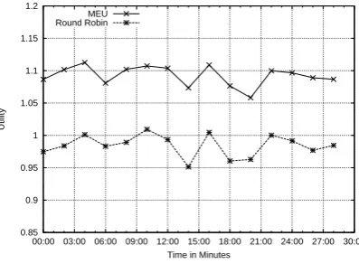
The taxonomy specifies that actions be chosen to maximise utility for single decision problems implemented using Bayesian decision networks. To judge the relative merit of the decision networks a round-robin action selection algorithm is also evaluated. The round robin algorithm cycles through the available phases at each junction running all phases consecutively and provides a good approximation of traditional fixed time junction controller strategies [23]. Fig. 13 shows the performance of the single-decision planning control units executed at each of the 247 junctions in the simulated city environment for each of the action selection algorithms. The data is displayed as a time series over 30 minutes. Each phase runs for 2 minutes as shown on the X axis. The Y axis shows the average reward across all junctions for the action selection algorithms over 15 phase decisions. The reward values shown on the Y axis are normalised so that the algorithms produce readings below 1. The normalised values for each algorithm are calculated as:PAvg AlgReward/PMEUMaxReward.PMEUMaxRewardis used as a normalisation factor across the result
320 340 360 380 400 420 440
140 160 180 200 220 240
Maximal Distance in kms
Degree of Interest ’500r_100t’
[image:21.595.71.522.119.610.2]’500r_500t’ ’500r_1000t’ ’500r_5000t’ "normalised_max"
Figure 9: CCTV Selection - SMOSA performance for 500 runs.
280 300 320 340 360 380 400 420 440
140 160 180 200 220 240
Maximal Distance in kms
Degree of Interest ’plot500r’ using 2:1
[image:21.595.66.271.131.275.2]"max" using 2:1
Figure 10: CCTV Selection - SA performance for 500 runs.
140
160 180
200
220 260 280
300 320 340 360
380 400 420 8 10 12 14 16 18 20 22 24
Number of Emergency Vehicles
"500r_500t" "normalised_max"
Degree of Interest
Maximal Distance in kms 8 10 12 14 16 18 20 22 24
Figure 11: CCTV Selection ext. - SMOSA performance for 500 runs. 120 140 160 180 200 220
240 260 280 300
320 340 360 380
400 420 8 10 12 14 16 18 20 22 24
Number of Emergency Vehicles
"500r" using 2:1:3 "max" using 2:1:3
Degree of Interest
Maximal Distance in kms 6 8 10 12 14 16 18 20 22
Figure 12: CCTV Selection ext. - SA performance for 500 runs.
0.85 0.9 0.95 1 1.05 1.1 1.15 1.2
00:00 03:00 06:00 09:00 12:00 15:00 18:00 21:00 24:00 27:00 30:00
Utility
Time in Minutes MEU
Round Robin
Figure 13: Junction Controller control unit performance.
0.85 0.9 0.95 1 1.05 1.1 1.15 1.2
00:00 03:00 06:00 09:00 12:00 15:00 18:00 21:00 24:00 27:00 30:00
Utility
Time in Minutes MEU
[image:21.595.324.523.489.635.2]Round Robin