Optimal Data Set Selection: An Application to Grapheme to Phoneme Conversion

Optimal Data Set Selection: An Application to Grapheme-to-Phoneme

Conversion

Young-Bum Kim and Benjamin Snyder University of Wisconsin-Madison {ybkim,bsnyder}@cs.wisc.edu

Abstract

In this paper we introduce the task of unla-beled, optimal, data set selection. Given a large pool of unlabeled examples, our goal is to select a small subset to label, which will yield a high performance supervised model over the entire data set. Our first proposed method, based on the rank-revealing QR ma-trix factorization, selects a subset of words which span the entire word-space effectively. For our second method, we develop the con-cept of feature coveragewhich we optimize with a greedy algorithm. We apply these methods to the task of grapheme-to-phoneme prediction. Experiments over a data-set of 8 languages show that in all scenarios, our selec-tion methods are effective at yielding a small, but optimal set of labelled examples. When fed into a state-of-the-art supervised model for grapheme-to-phoneme prediction, our meth-ods yield average error reductions of 20% over randomly selected examples.

1 Introduction

Over the last 15 years, supervised statistical learning has become the dominant paradigm for building nat-ural language technologies. While the accuracy of supervised models can be high, expertly annotated data sets exist for a small fraction of possible tasks, genres, and languages. The would-be tool builder is thus often faced with the prospect of annotating data, using crowd-sourcing or domain experts. With limited time and budget, the amount of data to be an-notated might be small, especially in the prototyping stage, when the exact specification of the prediction

task may still be in flux, and rapid prototypes are desired.

In this paper, we propose the problem of unsuper-vised, optimal data set selection. Formally, given a large set X of n unlabeled examples, we must select a subset S ⊂ X of size k n to label. Our goal is to select such a subset which, when labeled, will yield a high performance supervised model over the entire data setX. This task can be thought of as a zero-stage version of active learn-ing: we must choose a single batch of examples to label, without the benefit of any prior labelled data points. This problem definition avoids the practical complexity of the active learning set-up (many it-erations of learning and labeling), and ensures that the labeled examples are not tied to one particular model class or task, a well-known danger of active learning (Settles, 2010). Alternatively, our methods may be used to create the initial seed set for the ac-tive learner.

Our initial testbed for optimal data set selec-tion is the task of grapheme-to-phoneme conver-sion. In this task, we are given an out-of-vocabulary word, with the goal of predicting a sequence of phonemes corresponding to its pronunciation. As training data, we are given a pronunciation dic-tionary listing words alongside corresponding se-quences of phones, representing canonical pronun-ciations of those words. Such dictionaries are used as the final bridge between written and spoken lan-guage for technologies that span this divide, such as speech recognition, text-to-speech generation, and speech-to-speech language translation. These dic-tionaries are necessary: the pronunciation of words

continues to evolve after their written form has been fixed, leading to a large number of rules and ir-regularities. While large pronunciation dictionaries of over 100,000 words exist for several major lan-guages, these resources are entirely lacking for the majority of the world’s languages. Our goal is to automatically select a small but optimal subset of words to be annotated with pronunciation data.

The main intuition behind our approach is that the subset of selected data points should efficiently cover the range of phenomena most commonly ob-served across the pool of unlabeled examples. We consider two methods. The first comes from a line of research initiated by the numerical linear algebra community (Golub, 1965) and taken up by computer science theoreticians (Boutsidis et al., 2009), with the name COLUMNSUBSETSELECTIONPROBLEM (CSSP). Given a matrixA, the goal of CSSP is to se-lect a subset ofkcolumns whose span most closely captures the range of the full matrix. In particu-lar, the matrix A˜ formed by orthogonally project-ingAonto thek-dimensional space spanned by the selected columns should be a good approximation toA. By definingAT to be our data matrix, whose rows correspond to words and whose columns corre-spond to features (character 4-grams), we can apply the CSSP randomized algorithm of (Boutsidis et al., 2009) onAto obtain a subset ofkwords which best span the entire space of words.

Our second approach is based on a notion of fea-ture coverage. We assume that the benefit of seeing a feature f in a selected word bears some positive relationship to the frequency of f in the unlabeled pool. However, we further assume that the lion’s share of benefit accrues the first few times that we label a word with featuref, with the marginal util-ity quickly tapering off as more such examples have been labeled. We formalize this notion and provide an exact greedy algorithm for selecting the k data points with maximal feature coverage.

To assess the benefit of these methods, we ap-ply them to a suite of 8 languages with pronunci-ation dictionaries. We consider ranges from 500 to 2000 selected words and train a start-of-the-art grapheme-to-phoneme prediction model (Bisani and Ney, 2008). Our experiments show that both meth-ods produce significant improvements in prediction quality over randomly selected words, with our

fea-ture coverage method consistently outperforming the randomized CSSP algorithm. Over the 8 lan-guages, our method produces average reductions in error of 20%.

2 Background

Grapheme-to-phoneme Prediction The task of grapheme-to-phoneme conversion has been consid-ered in a variety of frameworks, including neural networks (Sejnowski and Rosenberg, 1987), rule-based FSA’s (Kaplan and Kay, 1994), and pronun-ciation by analogy (Marchand and Damper, 2000). Our goal here is not to compare these methods, so we focus on the probabilistic joint-sequence model of Bisani and Ney (2008). This model defines a joint distribution over a grapheme sequenceg∈G∗

and a phoneme sequence φ ∈ Φ∗, by way of an unobservedco-segmentationsequence q. Each co-segmentation unitqi is called agraphone and con-sists of an aligned pair of zero or one graphemes and zero or one phonemes:qi∈G∪ {} ×Φ∪ {}.1 The probability of a joint grapheme-phoneme sequence is then obtained by summing over all possible co-segmentations:

P(g,φ) = X

q∈S(g,φ)

P(q)

where S(g,φ) denotes the set of all graphone se-quences which yieldg andφ. The probability of a graphone sequence of lengthK is defined using an

h-order Markov model with multinomial transitions:

P(q) =

k+1

Y

i=1

P(qi|qi−h, . . . , qi−1)

where special start and end symbols are assumed for

qj<1andqk+1, respectively.

To deal with the unobserved co-segmentation se-quences, the authors develop an EM training regime that avoids overfitting using a variety of smoothing and initialization techniques. Their model produces state-of-the-art or comparable accuracies across a

1

wide range of languages and data sets.2 We use the publicly available code provided by the authors.3 In all our experiments we set h = 4 (i.e. a 5-gram model), as we found that accuracy tended to be flat forh >4.

Active Learning for G2P Perhaps most closely related to our work are the papers of Kominek and Black (2006) and Dwyer and Kondrak (2009), both of which use active learning to efficiently bootstrap pronunciation dictionaries. In the former, the au-thors develop an active learning word selection strat-egy for inducing pronunciation rules. In fact, their greedy n-gram selection strategy shares some of the some intuition as our second data set selection method, but they were unable to achieve any accu-racy gains over randomly selected words without ac-tive learning.

Dwyer and Kondrak use a Query-by-Bagging active learning strategy over decision tree learn-ers. They find that their active learning strategy produces higher accuracy across 5 of the 6 lan-guages that they explored (English being the ex-ception). They extract further performance gains through various refinements to their model. Even so, we found that the Bisani and Ney grapheme-to-phoneme (G2P) model (Bisani and Ney, 2008) al-ways achieved higher accuracy, even when trained on random words. Furthermore, the relative gains that we observe using our optimal data set selection strategies (without any active learning) are much larger than the relative gains of active learning found in their study.

Data Set Selection and Active Learning

Eck et al (2005) developed a method for train-ing compact Machine Translation systems by selecting a subset of sentences with high n-gram coverage. Their selection criterion essentially cor-responds to our feature coverage selection method using coverage function cov2 (see Section 3.2). As

our results will show, the use of a geometric feature discount (cov3) provided better results in our task.

Otherwise, we are not aware of previous work

2

We note that the discriminative model of Jiampojamarn and Kondrak (2010) outperforms the Bisani and Ney model by an average of about 0.75 percentage points across five data sets.

3_{http://www-i6.informatik.rwth-aachen.}

de/web/Software/g2p.html

proposing optimal data set selection as a general re-search problem. Of course, active learning strategies can be employed for this task by starting with a small random seed of examples and incrementally adding small batches. Unfortunately, this can lead to data-sets that are biased to work well for one particular class of models and task, but may otherwise perform worse than a random set of examples (Settles, 2010, Section 6.6). Furthermore the active learning set-up can be prohibitively tedious and slow. To illus-trate, Dwyer and Kondrak (2009) used 190 iterations of active learning to arrive at 2,000 words. Each iteration involves bootstrapping 10 different sam-ples, and training 10 corresponding learners. Thus, in total, the underlying prediction model is trained 1,900 times. In contrast, our selection methods are fast, can select any number of data points in a sin-gle step, and are not tied to a particular prediction task or model. Furthermore, these methods can be combined with active learning in selecting the initial seed set.

Unsupervised Feature Selection Finally, we note that CSSP and related spectral methods have been applied to the problem ofunsupervised feature se-lection(Stoppiglia et al., 2003; Mao, 2005; Wolf and Shashua, 2005; Zhao and Liu, 2007; Boutsidis et al., 2008). These methods are related to dimensionality reduction techniques such as Principal Components Analysis (PCA), but instead of truncating features in the eigenbasis representation (where each feature is a linear combination of all the original features), the goal is to remove dimensions in the standard basis, leading to a compact set of interpretable features. As long as the discarded features can be well approxi-mated by a (linear) function of the selected features, the loss of information will be minimal.

(a) (b) (c)

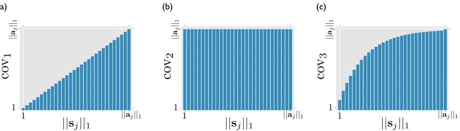
Figure 1: Various versions of the feature coverage function. Panel (a) shows cov1(Equation 5). Panel (b) shows cov2 (Equation 6). Panel (c) shows cov3(Equation 7) with discount factorη= 1.2.

3 Two Methods for Optimal Data Set Selection

In this section we detail our two proposed methods for optimal data set selection. The key intuition is that we would like to pick a subset of data points which broadly and efficiently cover the features of the full range of data points. We assume a large pool X ofn unlabeled examples, and our goal is to se-lect a subset S ⊂ X of size k n for labeling. We assume that each data point x ∈ X is a vec-tor ofmfeature values. Our first method applies to any real or complex feature space, while our second method is specialized for binary features. We will use the (n×m) matrixAto denote our unlabeled data: each row is a data point and each column is a feature. In all our experiments, we used the pres-ence (1) or abspres-ence (0) of each character 4-gram as our set of features.

3.1 Method 1: Row Subset Selection

To motivate this method, first consider the task of finding a rankkapproximation to the data matrixA. The SVD decomposition yields:

A=UΣVT

• U is(n×n)orthogonal and its columns form the eigenvectors ofAAT

• V is(m×m)orthogonal and its columns form the eigenvectors ofATA

• Σis(n×m)diagonal, and its diagonal entries are the singular values ofA(the square roots of the eigenvalues of bothAAT andATA).

To obtain a rankkapproximation toA, we start by rewriting the SVD decomposition as a sum:

A=

ρ X

i=1

σiuivTi (1)

whereρ= min(m, n),σiis the ithdiagonal entry of

Σ,uiis the ithcolumn ofU, andviis the ithcolumn ofV. To obtain a rank k approximation toA, we simply truncate the sum in equation 1 to its firstk

terms, yieldingAk. To evaluate the quality of this approximation, we can measure the Frobenius norm of the residual matrix ||A −Ak||F.4 The Eckart-Young theorem (Eckart and Eckart-Young, 1936) states that

Akis optimal in the following sense:

Ak= argmin

˜

A s.t.rank( ˜A)=k

||A−A˜||F (2)

In other words, truncated SVD gives the best rank

k approximation to A in terms of minimizing the Frobenius norm of the residual matrix. In CSSP, the goal is similar, with the added constraint that the approximation toAmust be obtained by projecting onto the subspace spanned by ak-subset of the orig-inal rows ofA.5 Formally, the goal is to produce a

(k×m)matrixSformed from rows ofA, such that

||A−AS+S||F (3)

4

The Frobenius norm||M||Fis defined as the entry-wiseL2 norm:qP

i,jm 2 ij 5

is minimized over all n_k

possible choices for S. Here S+ _{is the (m × k) Moore-Penrose}

pseudo-inverse ofS, andS+S gives the orthogonal projec-tor onto the rowspace ofS. In other words, our goal is to selectkdata points which serve as a good ap-proximate basis forallthe data points. SinceAS+S

can be at most rankk, the constraint considered here is stricter than that of Equation 1, so the truncated SVDAkgives a lower bound on the residual.

Boutsidis et al (2009) develop a randomized algo-rithm that produces a submatrix S (consisting ofk

rows ofA) which, with high probability, achieves a residual bound of:

||A−AS+S||F ≤O(k p

logk)||A−Ak||F (4)

in running time O(min{mn2, m2n}). The algo-rithm proceeds in three steps: first by computing the SVD of A, then by randomly sampling O(klogk)

rows of Awith importance weights carefully com-puted from the SVD, and then applying a determin-istic rank-revealing QR factorization (Golub, 1965) to selectk of the sampled rows. To give some in-tuition, we now provide some background on rank revealing factorizations.

Rank revealing QR / LQ (RRQR) Every real

(n×m)matrix can be factored asA=LQ, whereQ

is(m×m)orthogonal andLis(n×m)lower trian-gular.6It is important to notice that in this triangular factorization, each successive row of A introduces exactly one new basis vector fromQ. We can thus represent rowias a linear combination of the first

i−1rows along with the ithrow ofQ.

A rank-revealing factorization is one which dis-plays the numerical rank of the matrix — defined to be the singular value indexrsuch that

σr σr+1 =O()

for machine precision . In the case of the LQ

factorization, our goal is to order the rows of A

such that each successive row has decreasing rep-resentational importance as a basis for the future rows. More formally, If there exists a row permu-tationΠsuch thatΠAhas a triangular factorization

6

We replace the standard upper triangular QR factorization with an equivalent lower triangular factorization LQ to focus intuition on the rowspace ofA.

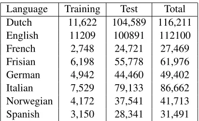
Language Training Test Total Dutch 11,622 104,589 116,211 English 11209 100891 112100 French 2,748 24,721 27,469 Frisian 6,198 55,778 61,976 German 4,942 44,460 49,402 Italian 7,529 79,133 86,662 Norwegian 4,172 37,541 41,713 Spanish 3,150 28,341 31,491

Table 1: Pronunciation dictionary size for each of the lan-guages.

ΠA = LQwith L = hL11 0 L21L22

i

, where the small-est singular value of L11 is much greater than the

spectral norm ofL22, which is itself almost zero:

σmin(L11) ||L22||2=O()

then we say thatΠA = LQis arank-revealing LQ factorization. Both L11 and L22 will be lower

tri-angular matrices and if L11 is (r ×r) then A has

numerical rankr(Hong and Pan, 1992).

Implementation In our implementation of the CSSP algorithm, we first prune away 4-gram fea-tures that appear in fewer than 3 words, then com-pute the SVD of the pruned data matrix using the PROPACK package,7 which efficiently handles sparse matrixes. After samplingklogkwords from

A(with sampling weights calculated from the top-k

singular vectors), we form a submatrix B consist-ing of the sampled words. We then use the RRQR implementation from ACM Algorithm 782 (Bischof and Quintana-Ort´ı, 1998) (routine DGEQPX) to compute ΠB = LQ. We finally select the first k

rows ofΠB as our optimal data set. Even for our largest data sets (English and Dutch), this entire pro-cedure runs in less than an hour on a 3.4Ghz quad-core i7 desktop with 32 GB of RAM.

3.2 Method 2: Feature Coverage Maximization

In our previous approach, we adopted a general method for approximating a matrix with a subset of rows (or columns). Here we develop a novel objec-tive function with the specific aim of optimal data set selection. Our key assumption is that the benefit of

7

seeing a new featuref in a selected data point bears a positive relationship to the frequency off in the unlabeled pool of words. However, we further as-sume that the lion’s share of benefit accrues quickly, with the marginal utility quickly tapering off as we label more and more examples with featuref. Note that for this method, we assume a boolean feature space.

To formalize this intuition, we will define the cov-erageof a selected(k×m)submatrixS consisting of rows ofA, with respect to a feature indexj. For il-lustration purposes, we will list three alternative def-initions:

cov1(S;j) =||sj||1 (5)

cov2(S;j) =||aj||1I ||sj||1>0

(6)

cov3(S;j) =||aj||1−

||aj||1

η||sj||1 I ||sj||1<||aj||1

(7)

In all cases,sj refers thejth column ofS,aj refers thejthcolumn ofA,I(·)is a 0-1 indicator function, andηis a scalar discount factor.8

Figure 1 provides an intuitive explanation of these functions: cov1 simply counts the number of

se-lected data points with boolean featurej. Thus, full coverage (||aj||: the entire number of data points with the feature) is only achieved when all data points with the feature are selected. cov2lies at the

opposite extreme. Even a single selected data point with featurejtriggers coverage of the entire feature. Finally, cov3 is designed so that the coverage scales

monotonically as additional data points with feature

jare selected. The first selected data point will cap-ture all but _η1 of the total coverage, and each further selected data point will capture all but 1_η of what-ever coverage remains. Essentially, the coverage for a feature scales as a geometric series in the number of selected examples having that feature.

To ensure that the total coverage (k|aj||1) is

achieved when all the data points are selected, we add an indicator function for the case of||cj||1 =

||aj||1.9

8

Chosen to be 5 in all our experiments. We experimented with several values between 2 and 10, without significant dif-ferences in results.

9_{Otherwise, the geometric coverage function would} con-verge to||aj||only as||cj|| → ∞.

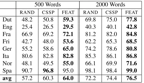
500 Words 2000 Words RAND CSSP FEAT RAND CSSP FEAT Dut 48.2 50.8 59.3 69.8 75.0 77.8

Eng 25.4 26.5 29.5 40.3 40.1 42.8

Fra 66.9 69.2 72.1 81.2 82.0 84.8

Fri 42.7 48.0 53.6 62.2 65.3 68.5

Ger 55.2 58.6 65.0 74.2 78.6 80.8

Ita 80.6 82.8 82.8 85.3 86.1 86.8

Nor 48.1 49.5 55.0 66.1 69.9 71.6

Spa 90.7 96.8 95.0 98.1 98.4 99.0 avg 57.2 60.3 64.0 72.2 74.4 76.5

Table 2: Test word accuracy across the 8 languages for randomly selected words (RAND), CSSP matrix subset selection (CSSP), and Feature Coverage Maximization (FEAT). We show results for 500 and 2000 word train-ing sets.

Setting our feature coverage function to cov3, we

can now define the overall feature coverage of the selected points as:

coverage(S) = 1

||A||1

X

j

cov3(S;j) (8)

where ||A||1 is the L1 entrywise matrix norm,

P

i,j|Aij|, which ensures that0≤coverage(S)≤

1 with equality only achieved when S = A, i.e. when all data points have been selected.

We provide a brief sketch of our optimization al-gorithm: To pick the subset S of k words which optimizes Equation 8, we incrementally build opti-mal subsetsS0 ⊂ S of sizek0 < k. At each stage, we keep track of the unclaimed coverage associated with each featurej:

unclaimed(j) =||aj||1−cov3(S0;j)

To add a new word, we scan through the pool of re-maining words, and calculate the additional cover-age that selecting wordwwould achieve:

∆(w) = X

featurejinw

unclaimed(j)

η−1 η

500 1000 1500 2000 25

30 35 40

English

500 1000 1500 2000 70

75 80

85

French

500 1000 1500 2000 90

92 94 96 98

Spanish

500 1000 1500 2000 80

81 82 83 84 85 86

87

Italian

500 1000 1500 2000 55

6065 70 75

80

German

500 1000 1500 2000 50

55 60 65

70

Norwegian

500 1000 1500 2000 5055

60 65 7075

80

Dutch

500 1000 1500 2000 45

50 55 60 65

70

Frisian

Feat Coverage

RRQR

Random

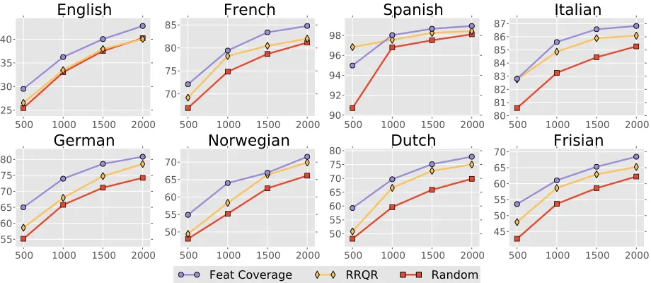
Figure 2: Test word accuracy across the 8 languages for (1) feature coverage, (2) CSSP matrix subset selection, (3) and randomly selected words.

4 Experiments and Analysis

To test the effectiveness of the two proposed data set selection methods, we conduct grapheme-to-phoneme prediction experiments across a test suite of 8 languages: Dutch, English, French, Frisian, German, Italian, Norwegian, and Spanish. The data was obtained from the PASCAL Letter-to-Phoneme Conversion Challenge,10 _{and was processed to} match the setup of Dwyer and Kondrak (2009). The data comes from a range of sources, includ-ing CELEX for Dutch and German (Baayen et al., 1995), BRULEX for French (Mousty et al., 1990), CMUDict for English,11 the Italian Festival Dictio-nary (Cosi et al., 2000), as well as pronunciation dic-tionaries for Spanish, Norwegian, and Frisian (orig-inal provenance not clear).

As Table 1 shows, the size of the dictionaries ranges from 31,491 words (Spanish) up to 116,211 words (Dutch). We follow the PASCAL challenge training and test folds, treating the training set as our pool of words to be selected for labeling.

Results We consider training subsets of sizes 500, 1000, 1500, and 2000. For our baseline, we train the

10_{http://pascallin.ecs.soton.ac.uk/}

Challenges/PRONALSYL/

11_{http://www.speech.cs.cmu.edu/cgi-bin/}

cmudict

G2P model (Bisani and Ney, 2008) on randomly se-lected words of each size, and average the results over 10 runs. We follow the same procedure for our two data set selection methods. Figure 2 plots the word prediction accuracy for all three meth-ods across the eight languages with varying training sizes, while Table 2 provides corresponding numer-ical results. We see that in all scenarios the two data set selection strategies fare better than random sub-sets of words.

In all but one case, the feature coverage method yields the best performance (with the exception of Spanish trained with 500 words, where the CSSP yields the best results). Feature coverage achieves average error reduction of 20% over the randomly selected training words across the different lan-guages and training set sizes.

Coverage variants We also experimented with the other versions of the feature coverage function discussed in Section 3.2 (see Figure 1). While cov1

tended to perform quite poorly (usually worse than random), cov2 — which gives full credit for each

feature the first time it is seen — yields results just slightly worse than the CSSP matrix method on av-erage, and always better than random. In the 2000 word scenario, for example, cov2 achieves average

RAND CSSP FEAT SVD Fra 0.66 0.62 0.65 0.51 Fry 0.75 0.72 0.75 0.6 Ger 0.71 0.67 0.71 0.55 Ita 0.64 0.61 0.67 0.49 Nor 0.7 0.61 0.64 0.5 Spa 0.65 0.67 0.68 0.53

avg 0.69 0.65 0.68 0.53

Table 3: Residual matrix norm across 6 languages for randomly selected words (RAND), CSSP matrix subset selection (CSSP), feature coverage maximization (FEAT), and the rankkSVD (SVD). Lower is better.

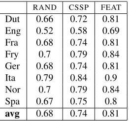
RAND CSSP FEAT Dut 0.66 0.72 0.81 Eng 0.52 0.58 0.69 Fra 0.68 0.74 0.81 Fry 0.7 0.79 0.84 Ger 0.68 0.74 0.81 Ita 0.79 0.84 0.9 Nor 0.7 0.79 0.84 Spa 0.67 0.75 0.8

avg 0.68 0.74 0.81

Table 4: Feature coverage across the 8 languages for ran-domly selected words (RAND), CSSP matrix subset selec-tion (CSSP), and feature coverage maximizaselec-tion (FEAT). Higher is better.

careful tuning of the discount factorηof cov3would

yield further gains.

Optimization Analysis Both the CSSP and fea-ture coverage methods have clearly defined objec-tive functions — formulated in Equations 3 and 8, respectively. We can therefore ask how well each methods fares in optimizing either one of the two objectives.

First we consider the objective of the CSSP al-gorithm: to findkdata points which can accurately embed the entire data matrix. Once the data points are selected, we compute the orthogonal projection of the data matrix onto the submatrix, obtaining an approximation matrixA˜. We can then measure the residual norm as a fraction of the original matrix norm:

||A−A˜||F

||A||_F (9)

As noted in Section 3.1, truncated SVD minimizes the residual over all rankkmatrices, so we can

com-CSSP FEAT FEAT-SLS

fettered internationalization rating exceptionally underestimating overs gellert schellinger nation daughtry barristers scherman blowed constellations olinger harmonium complementing anderson cassini bergerman inter rupees characteristically stated tewksbury heatherington press ley overstated conner

Table 5: Top 10 words selected by CSSP, feature cov-erage (FEAT), and feature covcov-erage with stratified length sampling (FEAT-SLS)

pare our three methods — random selections, CSSP, and feature coverage — all of which selectk exam-ples as a basis, against the lower bound given by SVD. Table 3 shows the result of this analysis for

k = 2000 (Note that we were unable to compute the projection matrices for English and Dutch due to the size of the data and memory limitations). As expected, SVD fares the best, with CSSP as a some-what distant second. On average, feature coverage seems to do a bit better than random.

A similar analysis for the feature coverage objec-tive function is shown in Table 4. Unsurprisingly, this objective is best optimized by the feature cov-erage method. Interestingly though, CSSP seems to perform about halfway between random and the feature coverage method. This makes some sense, as good basis data points will tend to have frequent features, while at the same time being maximally spread out from one another. We also note that the poor coverage result for English in Table 4 mir-rors its overall poor performance in the G2P predic-tion task – not only are the phoneme labels unpre-dictable, but the input data itself is wild and hard to compress.

according to the feature coverage criterion. This re-sults in more typical words of average length, with only a very small drop in performance.

5 Conclusion and Future Work

In this paper we proposed the task of optimal data set selection in the unsupervised setting. In contrast to active learning, our methods do not require re-peated training of multiple models and iterative an-notations. Since the methods are unsupervised, they also avoid tying the selected data set to a particular model class (or even task).

We proposed two methods for optimally select-ing a small subset of examples for labelselect-ing. The first uses techniques developed by the numerical lin-ear algebra and theory communities for approximat-ing matrices with subsets of columns or rows. For our second method, we developed a novel notion of feature coverage. Experiments on the task of grapheme-to-phoneme prediction across eight lan-guages show that our method yields performance improvements in all scenarios, averaging 20% re-duction in error. For future work, we intend to apply the data set selection strategies to other NLP tasks, such as the optimal selection of sentences for tag-ging and parsing.

Acknowledgments

The authors thank the reviewers and acknowledge support by the NSF (grant IIS-1116676) and a re-search gift from Google. Any opinions, findings, or conclusions are those of the authors, and do not nec-essarily reflect the views of the NSF.

References

RH Baayen, R. Piepenbrock, and L. Gulikers. 1995. The celex lexical database (version release 2)[cd-rom]. Philadelphia, PA: Linguistic Data Consortium, Uni-versity of Pennsylvania.

Maximilian Bisani and Hermann Ney. 2008. Joint-sequence models for grapheme-to-phoneme conver-sion.Speech Communication, 50(5):434–451, 5. C.H. Bischof and G. Quintana-Ort´ı. 1998. Algorithm

782: codes for rank-revealing qr factorizations of dense matrices. ACM Transactions on Mathematical Software (TOMS), 24(2):254–257.

C. Boutsidis, M.W. Mahoney, and P. Drineas. 2008. Un-supervised feature selection for principal components

analysis. In Proceeding of the 14th ACM SIGKDD international conference on Knowledge discovery and data mining, pages 61–69.

C. Boutsidis, M. W. Mahoney, and P. Drineas. 2009. An improved approximation algorithm for the column subset selection problem. InProceedings of the twen-tieth Annual ACM-SIAM Symposium on Discrete Al-gorithms, pages 968–977. Society for Industrial and Applied Mathematics.

P. Cosi, R. Gretter, and F. Tesser. 2000. Festival parla italiano. Proceedings of GFS2000, Giornate del Gruppo di Fonetica Sperimentale, Padova.

K. Dwyer and G. Kondrak. 2009. Reducing the anno-tation effort for letter-to-phoneme conversion. In Pro-ceedings of the ACL, pages 127–135. Association for Computational Linguistics.

Matthias Eck, Stephan Vogel, and Alex Waibel. 2005. Low cost portability for statistical machine translation based on n-gram coverage. InProceedings of the Ma-chine Translation Summit X.

C. Eckart and G. Young. 1936. The approximation of one matrix by another of lower rank. Psychometrika, 1(3):211–218.

G. Golub. 1965. Numerical methods for solving lin-ear least squares problems. Numerische Mathematik, 7(3):206–216.

Yoo Pyo Hong and C-T Pan. 1992. Rank-revealing factorizations and the singular value decomposition. Mathematics of Computation, 58(197):213–232. S. Jiampojamarn and G. Kondrak. 2010. Letter-phoneme

alignment: An exploration. In Proceedings of the ACL, pages 780–788. Association for Computational Linguistics.

R.M. Kaplan and M. Kay. 1994. Regular models of phonological rule systems.Computational linguistics, 20(3):331–378.

J. Kominek and A. W. Black. 2006. Learning pronunci-ation dictionaries: language complexity and word se-lection strategies. InProceedings of the NAACL, pages 232–239. Association for Computational Linguistics. K.Z. Mao. 2005. Identifying critical variables of

prin-cipal components for unsupervised feature selection. Systems, Man, and Cybernetics, Part B: Cybernetics, IEEE Transactions on, 35(2):339–344.

Y. Marchand and R.I. Damper. 2000. A multistrategy ap-proach to improving pronunciation by analogy. Com-putational Linguistics, 26(2):195–219.

P. Mousty, M. Radeau, et al. 1990. Brulex. une base de donn´ees lexicales informatis´ee pour le franc¸ais ´ecrit et parl´e.L’ann´ee psychologique, 90(4):551–566. T.J. Sejnowski and C.R. Rosenberg. 1987. Parallel

Burr Settles. 2010. Active learning literature survey. Technical Report TR1648, Department of Computer Sciences, University of Wisconsin-Madison.

H. Stoppiglia, G. Dreyfus, R. Dubois, and Y. Oussar. 2003. Ranking a random feature for variable and fea-ture selection. The Journal of Machine Learning Re-search, 3:1399–1414.

L. Wolf and A. Shashua. 2005. Feature selection for un-supervised and un-supervised inference: The emergence of sparsity in a weight-based approach. The Journal of Machine Learning Research, 6:1855–1887. Z. Zhao and H. Liu. 2007. Spectral feature selection for