Munich Personal RePEc Archive
A simple model of time zone differences,
virtual trade and informality
Mandal, Biswajit and Prasad, Alaka Shree
Department of Economics and Politics, Visva-Bharati University,
Santiniketan, India, 731235
2018
Online at
https://mpra.ub.uni-muenchen.de/96953/
A SIMPLE MODEL OF TIME ZONE DIFFERENCES, VIRTUAL TRADE
AND INFORMALITY
Biswajit Mandal
Department of Economics & Politics, Visva-Bharati University, Santiniketan, India, 731235
Email: [email protected]
Alaka Shree Prasad
Department of Economics & Politics, Visva-Bharati University Santiniketan, India, 731235
Email: [email protected]
Corresponding author:
Biswajit Mandal
Department of Economics & Politics Visva-Bharati University
Santiniketan, India 731235
ABSTRACT
In this paper we attempt to model virtual trade resulting from time zone differences in an
otherwise Heckscher-Ohlin set up which is absent in the literature. So, this paper tries to add
some value to the existing stuff on the trade theory and the role of time zones. In doing so, it has
been proved that exploitation of time zone difference benefits skilled labor only under reasonable
assumption. Contrarily, in output font, time zone difference exploiting sector expands and the
other sector contracts irrespective of any factor intensity assumption. The model has been
extended to examine how distance may also lead to similar outcomes. In addition, the model is
further extended to explore the effect of virtual trade on an economy also endowed with a huge
supply of unskilled labor causing the occurrence of informality and associated corruption.
Interestingly trade turns out to be beneficial to unskilled workers and lead to a fall in the number
of workers engaged in corrupt activities in the economy though the informal sector expands.
JEL Classification: F1, F11, E26, J31, D73
1
1
Introduction
Very recently the composition of trade has changed to a significant extent in favor of
exchange of services predominantly done ‘virtually’ in a sense. Virtual trade1 mainly includes
business services such as engineering, software development, call centre, insurance claim
settlements, medical advice etc. This type of trade provides us the opportunity of utilizing time
zone difference beneficially by adopting the time saving, follow-the-sun system of service
provision/development.2 The creation of service is divided into multiple sequential stages and
assigned to groups located in different time zones. The process is accomplished with each group
working in regular office hours on the allotted task, and transferring the same to the other group
at the end of their working hours. One common element of all such activities is the non
requirement of physical transportation of the product, be it intermediate or final, and non
requirement of physical presence of sellers and buyers at the time of transaction. But it certainly
requires high bandwidth internet or Information Communication Technology (ICT). Thanks to
the information technology revolution the cost of ICT has gone down drastically making room
for virtual transaction to be done almost costlessly. To exploit this possibility, however, time
zones (TZ) of trading partners or countries must be non-overlapping3. This issue has been
explained very nicely in Marjit (2007), Kikuchi (2011), Kikuchi and Marjit (2011), Kikuchi et al.
(2013), Anderson (2014), Dettmer (2014), Head et al. (2009), Matsuoka and Fukushima (2010),
Nakanishi and Long (2015), Mandal et al. (2018b), Fink et al. (2005), Mandal (2015), Marjit and
Mandal (2017) etc.4 For the purpose of current essay we focus only on the cost associated with
delay in delivery that can be avoided when virtual trade is appropriated. Kikuchi (2006) and
Marjit (2007) are two papers that deal with such concern. Although issues in and around this
1
Virtual trade refers to the exchange of services done using the communication technology like e-mail, teleconferencing, video conferencing and many other information sharing tools.
2For example, India’s service sector has grown rapidly after liberalization and this is particularly because of
software exports whose transactions require a virtual platform. Marjit and Mandal (2017) points out that this growth
in service exports is to a great extent a result of India’s geographical location which makes it to be in a different time
zone from its major partners.
3
By non-overlapping time zone we mean, one country’s day does not coincide with the other i.e. when there is day in one country its night in the other. If time zones are non-overlapping, working hours are also different. In this paper, we have considered working hours to be of 12 hours, so the terms non-overlapping time zones and non- overlapping working hours have been used interchangeably.
4
2
concern are gradually gaining more importance, to the best of our knowledge, we have not seen
any attempt to bring in time zone (TZ) related phenomena in a standard Heckscher-Ohlin kind of
general equilibrium model of trade (Jones, 1965). Therefore, this paper is a humble effort to fill
up this caveat. There are two formal sectors, and two factors—skilled labor and capital. The
model aims to find the effect of virtual trade on the two sectors and the involved factors. Virtual
trade alone does not depend on the distance as such, but when virtual trade occurs in order to
exploit the difference in time zones, east-west distance between the partners does matter. Mandal
(2015) briefly and nicely elaborates the relation between time zone difference and distance.
Following this paper we also try to incorporate distance in the proposed framework to examine
the effect of east-west distance on virtual trade that is undertaken to exploit the time zone
difference, and its subsequent effect on the economy.
Another important issue which is a major concern in many developing parts of the world is
the presence of informality in the economy. The issue becomes more serious when informal
sector is beset with corrupt activities. Informality could be described in many different ways. In
this paper we consider the view points of Marjit and Kar (2011), Mandal (2011), Mandal et al
(2018a) etc. Following these papers, informal sector arise as the formal sector cannot absorb the
entire labor pool available in the economy. In order to survive these people organize some
productive units which are not formal in nature. This means they violate some government rules,
they are not registered, they do not pay tax, do not follow minimum wage regulations, their wage
is less compared to the formal sector, etc. It has also been observed that because of their
illegal/extralegal nature extortionists exploit them and collect extortion fees (see Mandal et al.,
2018a). These extortionists are unproductive in line with Bhagwati (1982). However, they save
these informal units whenever they are trapped in legal issues by negotiating with the legal
authorities. Therefore, the informal sector cannot get rid of these corrupt people and have to pay
a part of their income to these intermediaries. So, this paper is also extended by considering
some unpraised aspects of developing economies—huge supply of unskilled labor, presence of
informal sector and informality related corruption—in the constructed framework and tries to
figure out whether the effect of trade driven by non-overlapping time zones benefits the
economy.
Remaining paper is arranged as follows. Section 2 builds the basic model using
3
sectors opts for trade across different TZs. Output of the sector engaged in virtual trade expands
while that of the other sector contracts. Similarly, return to the factor used intensively in the
production of TZ utilizing sector rises and the return to the factor used intensively in the other
sector falls. Section 3 introduces distance in the model and shows its impact on factor prices and
output. The results are seen to be analogous to the previous section indicating a positive effect of
distance. In section 4 the model is further extended to a four sector-three factor economy, where
we introduce informality using the difference between pre-negotiated fixed and variable wage for
unskilled labor (Marjit and Kar, 2011).The objective of the extension is to see whether time zone
differences help to truncate the intermediation sector that provides support to the informal
production units. Finally, section 5 concludes the paper. Mathematical derivations are, however,
relegated to the Appendices.
2
The Basic Model
We consider two countries and rest of the world. The two countries are identical in all
respect except their geographical locations on the globe. They are located in such a way that their
time zones are completely non-overlapping. Since the two countries are identical, both will
experience the same kind of effect. Therefore, we focus on only one country. The concerned
economy produces two commodities 𝑋 and 𝑌. 𝑋 is a service while 𝑌 is a tangible good. Each
good is produced using skilled labor (𝑆) and capital (𝐾) under constant returns to scale (CRS)
and diminishing marginal productivity (DMP) of factors and are sold in a perfectly competitive
market.5 Markets open in every 24 hours. Prices are set in the world market and the economy
which we consider to be small cannot alter them. To produce a unit of 𝑌, 𝑎𝑆𝑌 units of skilled labor and 𝑎𝐾𝑌 units of capital are engaged. Production is accomplished in one working day. One working day consists of 12 hours of work during daytime; the night time is the leisure time.
Production of 𝑋 requires 24 hours of work. Therefore, following Marjit (2007) we assume the
5
The symbols that has been used in this paper are given as follows: 𝑆= (total supply of) skilled labor; 𝐾= (total supply of) capital; 𝐿= (total supply of) unskilled labor; 𝑋= service output; 𝑌= physical good produced in formal environment; 𝑍= informal sector output; 𝑁= corrupt sector; 𝐿𝑁= total amount of 𝐿 engaged in 𝑁; 𝑎𝑖𝑗 =amount of 𝑖𝑡ℎ factor used in production of one unit of 𝑗𝑡ℎ commodity (𝑖=𝑆,𝐾,𝐿 and 𝑗=𝑋,𝑌,𝑍,𝑁); 𝑤𝑠= wage of skilled labor;
𝑤= wage of unskilled labor; 𝑤 = unionized wage; 𝑟= rent; 𝑃𝑗= price of 𝑗𝑡ℎ commodity; 𝛿= the discount factor;
𝜃𝑖𝑗= distributive share of 𝑖𝑡ℎ factor in 𝑗𝑡ℎ commodity; 𝜆𝑖𝑗 = employment share of 𝑖𝑡ℎ factor in 𝑗𝑡ℎ commodity; 𝜎𝑌=
4
production of 𝑋 to be divided into two stages; each stage requiring one working day and each
working day utilizing one unit of both labor and capital. Thus the service is ready, engaging two
units of labor and capital, in two days and the consumer receives it on the third day. With this
much time taken for production and delivery the price that the producer receives is 𝛿𝑃𝑋, with 𝑃𝑋
being the price of 𝑋 and 𝛿 the discount factor. The discount factor 𝛿 (0 <𝛿 ≤1) captures the
time preference of the consumers. The consumers are eager to get the product earlier and for that
they are ready to pay more. So if the service is delivered late the value of 𝛿 falls and if it is
delivered earlier 𝛿 rises. As perfect competition exists per unit cost will be equal to its price.
Therefore, the cost-price equations are given by
2𝑤𝑆 + 2𝑟=𝛿𝑃𝑋 (1)
𝑤𝑆𝑎𝑆𝑌+𝑟𝑎𝐾𝑌 =𝑃𝑌 (2)
𝑤𝑆 and 𝑟 are wage and rent, respectively. 𝑃𝑋 and 𝑃𝑌 in the same way denote prices of good 𝑋 and
good 𝑌. The technological coefficients are fixed for the production of 𝑋 while 𝑎𝑆𝑌 and 𝑎𝐾𝑌, the
technological coefficients for 𝑌 production, are considered to be variable.6 In the concerned
economy skilled labor is used intensively in 𝑋 whereas 𝑌 is a capital intensive good. Factors are
fully employed within both the sectors.
The full employment equations are given by
2𝑋+𝑎𝑆𝑌𝑌=𝑆 (3)
2𝑋+𝑎𝐾𝑌𝑌 =𝐾 (4)
Solution of the model is quite well known in the trade literature. Interested readers may go
through Jones (1965). We have four unknown variables 𝑤𝑆,𝑟,𝑋and 𝑌to solve from equation
(1)–(4). Given commodity prices factor prices are determined from (1) and (2). Once factor prices are solved we have the values of technological coefficients through CRS assumption.
Once aijs are known we can calculate X and Y from (3) and (4). So, the system is solvable.
6
Technological coefficients are functions of factor prices and can change when there is any change in factor price. Here, this is possible for 𝑌 but not for 𝑋. The rationale comes from the assumption that the production of service takes two consecutive working days, each day requiring one unit of skilled labour and capital. Therefore, 2 units of
5
2.1. Effect of Utilization of Time Zone Differences
One way for the producers of 𝑋 to realize the full value of their service is to reduce the time
required for production. This can be achieved when production is fragmented between two
countries with non overlapping working hours i.e. situated in different time zones. With this,
production process continues for 24 hours as when working hours ends in one country, it starts in
the other. The first stage is produced within 12 hours of working day in one country and the
semi-finished task is delegated to the other country at the end of the day where the second stage
is completed. Thus production process takes two working days as before but because the process
is separated between non overlapping time zones, two working days are achieved within a single
calendar date. As a result consumers receive the product on the second day—one day earlier.
Following Mandal (2015), since the time zones of the two countries are completely
non-overlapping, this pushes up the value of 𝛿 to 1 and the producers obtain full value of the service.
This change of 𝛿 from less than 1 to equal to 1 benefits individual producers and also affects
factor prices and outputs.
2.1.1 Effect on Factor Prices
Taking total differential of equation (1) and (2), and expressing percentage change with ‘^’
we get,
𝑤 𝑆𝜃𝑆𝑋 +𝑟 𝜃𝐾𝑋 = 𝛿 𝛿 (5)
𝑤 𝑆𝜃𝑆𝑌+𝑟 𝜃𝐾𝑌 = 0 (6)
With a relatively high effective price (because of rise in𝛿) of X, as production of X
becomes more lucrative, demand for factors used in X increases. This increases the factor prices
in the economy. Since the price of 𝑌 has not changed, with rise in input prices, producing the
existing level of output becomes unviable for 𝑌 producers. 𝑌 reduces its output releasing skilled
labor and capital. 𝑌 being capital intensive releases more of 𝐾 than 𝑆. Released 𝑆 gets employed
in 𝑋 but all the released 𝐾 cannot. This leads to excess demand for 𝑆 and excess supply of 𝐾.
Eventually, wage rises and rent falls7. This result is quite apparent.
Using equation (5) and (6) we get the changes in wage and rent as (see Appendix A):
7
6
𝑤 𝑆 =𝛿 𝛿 𝜃 𝜃 𝐾𝑌 > 0 (7)
𝑟 = − 𝜃𝑆𝑌
𝜃 𝛿 𝛿< 0 (8)
𝜃 = 𝜃𝑆𝑋𝜃𝐾𝑌− 𝜃𝑆𝑌𝜃𝐾𝑋 > 0; since,𝜃𝑆𝑋 > 𝜃𝑆𝑌 and 𝜃𝐾𝑋 <𝜃𝐾𝑌
Note that the direction of changes depends on the factor intensity of the goods in addition to the
change in the discount rate. Thus we have the following proposition
Proposition 1: Exploitation of TZ differences benefits the factor used intensively in the service
sector while the other factor suffers a loss.
Proof: See discussion above.
2.1.2 Effect on Output
As 𝑌 production is characterized by variable coefficient technology, amount of factors
(labor and capital) used in its production can be altered and the relatively costly skilled labor can
be replaced by cheaper capital. To spot the variation in the coefficients we use elasticity of
substitution between two factors which is expressed as (for details see Appendix B)
𝜎𝑌= 𝑎 𝑆𝑌𝑟 − 𝑤− 𝑎 𝐾𝑌 𝑆
(9)
Using Envelope condition one gets
𝑎 𝐾𝑌 = − 𝜃𝜃𝑆𝑌 𝐾𝑌𝑎 𝑆𝑌
Substituting this in equation (9) and putting the value of(𝑟 − 𝑤𝑠), (relevant mathematical
expression is given in Appendix A) we get,
𝑎 𝑆𝑌 = − 𝛿𝛿 𝜃 𝜃 𝜎𝐾𝑌 𝑌 < 0 (10)
𝑎 𝐾𝑌 =𝛿𝛿 𝜃 𝜃 𝜎𝑆𝑌 𝑌 > 0 (11)
The above equations exhibit the change in the amount of factors employed in production
of one unit of 𝑌 when the other sector (𝑋) utilizes the time zone differences between two
7
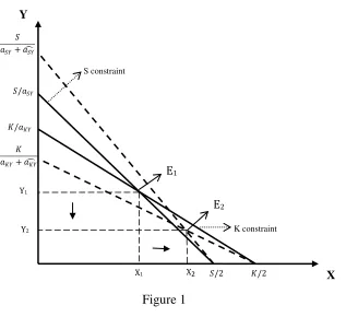
In Figure 1, equation (3) has been plotted as 𝑆 constraint while equation (4) has been
plotted as 𝐾 constraint. The initial equilibrium is shown to be at 𝐸1where the economy produces
𝑋1 and 𝑌1 units of 𝑋 and 𝑌, respectively. When effective price of 𝑋 rises because of the rise in 𝛿, the production of 𝑋 becomes more lucrative. As explained earlier, factor intensity assumptions
cause an excess demand for 𝑆and excess supply of 𝐾. As a result wage rises and rent falls. Since
factor requirements are function of factor prices, rise in wages leads to a fall in its usage in
production of one unit of 𝑌 (𝑎𝑆𝑌 < 0). On the other hand, per unit requirement of 𝐾 rises
(𝑎𝐾𝑌 > 0). We can see in Figure 1, change in 𝑎𝑆𝑌 and 𝑎𝐾𝑌 moves the labor and capital
constraints along the Y-axis which changes the equilibrium level of 𝑋 and 𝑌. 𝑆-constraint moves
outward while 𝐾-constraint moves inward. The new equilibrium is at 𝐸2, which shows higher
output of 𝑋 (at 𝑋2) and a lower 𝑌 (at 𝑌2). To mathematically elucidate the changes in the
equilibrium level of 𝑋 and 𝑌 we take total differential of (3) and (4)
𝑋 𝜆𝑆𝑋 +𝑌 𝜆𝑆𝑌+𝜆𝑆𝑌𝑎 𝑆𝑌 = 0
𝑋 𝜆𝐾𝑋 +𝑌 𝜆𝐾𝑌+𝜆𝐾𝑌𝑎 𝐾𝑌 = 0 X2
X1 Y2
Y1
E2 E1
𝑆 𝑎𝑆𝑌+𝑎𝑆𝑌
K constraint S constraint
𝐾/2 𝑆/2
𝐾 𝑎𝐾𝑌+𝑎𝐾𝑌
𝐾/𝑎𝐾𝑌 𝑆/𝑎𝑆𝑌 Y
[image:10.612.153.470.69.359.2]X
8
Substituting the values of 𝑎 𝑆𝑌 and 𝑎 𝐾𝑌 given by equation (10) and (11); and applying the Cramer’s rule (see Appendix C) we have
𝑋 = 1
𝜆
1
𝜃 𝜃𝐾𝑌𝜆𝑆𝑌𝜆𝐾𝑌+𝜃𝑆𝑌𝜆𝐾𝑌𝜆𝑆𝑌 𝜎𝑌𝛿𝛿 > 0 (12)
8
𝑌 = − 1
𝜆
1
𝜃 𝜃𝑆𝑌𝜆𝑆𝑋𝜆𝐾𝑌+𝜃𝐾𝑌𝜆𝐾𝑋𝜆𝑆𝑌 𝜎𝑌𝛿𝛿 < 0 (13)
Note that both 𝜆 and 𝜃 are positive owing to assumed factor intensity of 𝑋 and 𝑌.
𝑋 > 0 as 𝛿 > 0. This confirms that there is a rise in 𝑋 (as shown in Figure 1) due to utilization of
time zone difference. Correspondingly we experience a reduction in 𝑌. Interestingly, the
direction of change is independent of the factor intensity assumption as both 𝜆 and 𝜃 have the
same sign. Thus we have Proposition 2 as follows;
Proposition 2: Due to TZ difference exploitation 𝑋 expands and 𝑌 contracts irrespective of
factor intensity assumption. ▄
3
Extended Model with Distance
In Section 2 we have explained that value of 𝛿 falls if the service is delivered late.
Production and delivery can be done faster when time zone difference is utilized. It will be done
in minimum time when TZs of partner countries are completely non-overlapping. Alongside, two countries’ TZs become more and more non-overlapping when their distance9
becomes larger and
larger. Therefore, 𝛿 is a function of distance, 𝐷 (Mandal, 2015) i.e.
𝛿 =𝛿(𝐷) (14)
Taking total differential we have,
8 𝜆
= 𝜆𝑆𝑋 𝜆𝑆𝑌
𝜆𝐾𝑋 𝜆𝐾𝑌 and [ 𝜆𝑆𝑋 =
2𝑋
𝑆 ; 𝜆𝑆𝑌 = 𝑌𝑎𝑆𝑌
𝑆 ;𝜆𝐾𝑋 =
2𝑋
𝐾 ;𝜆𝐾𝑌= 𝑌𝑎𝐾𝑌
𝐾 ]
9
9 𝛿 =𝛿′ 𝐷 𝑑𝐷
𝛿 (15)
The above equation shows the relation between 𝛿 and distance. 𝛿′ 𝐷 is positive as with
rise in distance TZ differences can be exploited more aptly and 𝛿 rises to raise the effective
commodity price that is realized by the producer.
Now to see the effect of distance on factor prices and output of the economy we put the
value of 𝛿 in equation (7), (8), (12) and (13). The results are as shown below:
𝑤𝑠 =𝛿′ 𝐷 𝑑𝐷 𝜃 𝜃 𝐾𝑌 > 0
𝑟 = − 𝜃𝑆𝑌
𝜃 𝛿′ 𝐷 𝑑𝐷< 0
𝑋 = 1
𝜆
1
𝜃 𝜃𝐾𝑌𝜆𝑆𝑌𝜆𝐾𝑌 +𝜃𝑆𝑌𝜆𝐾𝑌𝜆𝑆𝑌 𝜎𝑌𝛿′ 𝐷 𝑑𝐷> 0
𝑌 = − 1
𝜆
1
𝜃 𝜃𝑠𝑦𝜆𝑆𝑋𝜆𝐾𝑌+𝜃𝑘𝑦𝜆𝐾𝑋𝜆𝑆𝑌 𝜎𝑌𝛿′ 𝐷 𝑑𝐷 < 0
So, the effects are similar to that in the previous section. However, the results contradict the
conventional understanding of the role of distance in trade as depicted by the gravity theory. This
is because, the reason for which distance was assumed to deter trade does not arise in our model.
In gravity model distance is taken to hinder trade as with rise in distance the transportation cost
and transaction cost also rises. However, in our model of service trade transporting services is
done virtually which is independent of distance between two countries. Secondly, the production
process is considered to be sequential so that interaction between the affiliates is rarely required.
Thus here we notice increasing distance to benefit the sector that undertakes trade across
significant distance.10 Rise in distance also leads to a positive change in wage rate and a negative
10
10
change in rent as before. The direction of change of factor prices is such, as skilled labor is
intensively used in 𝑋 relative to 𝑌.
4
Inclusion of Informal Sector
In this section we extend our model by adding an informal sector which is often present in
developing and even in developed countries (Mandal et al., 2018a). We follow Mandal et al.
(2018a), Mandal (2011), and Mandal and Chaudhuri (2011) where the informal sector consists of
a productive segment and a profit seeking directly unproductive unit as termed in Bhagwati
(1982). Informal segment of the economy exists violating some government prescribed rules for
example, they do not pay tax, are not registered, do not follow minimum wage law, exploit their
workers, occupy government land for production etc. Because of its extralegal nature whenever
legal issues arise they need to take help of some people who negotiate with the legal officials and
free them from penalizing charges. In return these people appropriate a part of the income of the
informal units.11 So, informal units suffer from extortion irrespective of whether the need for
intermediation arises or not. We term these people engaged in intermediation as extortionists or
intermediators. The extortionists get wage equal to the competitive wage of workers engaged in
the productive informal segment as labor is perfectly mobile between these activities. Again
informal wage is less than the formal wage where minimum wage rule is followed (for detailed
argument see Marjit and Kar (2011)). We consider corruption to be present only in informal
sector. Therefore, along with the sectors 𝑋 and 𝑌, there are two more sectors, 𝑍 and 𝑁. 𝑋 and 𝑌
are formal sectors, 𝑍 is an informal sector and 𝑁 sector helps the informal sector to subsist.
Further we assume now that there are three factors of production, skilled labor (𝑆), capital (𝐾)
and unskilled labour (𝐿), with sector 𝑋 using 𝑆 and 𝐾 as before; sector 𝑌 using 𝐿 at a
pre-negotiated wage rate along with 𝑆 and 𝐾; sector 𝑍 using 𝐿 and 𝐾 and finally sector 𝑁 using only
𝐿. Unskilled labor who do not get employed in 𝑌 has to survive by working in either 𝑍 or 𝑁. We assume sector 𝑍 to be unskilled labor intensive. In this backdrop, we try to check whether trade
across time zone differences has some effect on the size of informal sector and associated
corruption. This is our prime focus. We will, however, look at the effects on factor prices and
wage disparity between skilled and unskilled workers.
11
11
The modified price equations are given as:
2𝑤𝑆 + 2𝑟=𝛿𝑃𝑋 (16)
𝑎𝐿𝑌𝑤 + 𝑤𝑆𝑎𝑆𝑌 +𝑟𝑎𝐾𝑌 =𝑃𝑌 (17)
𝑎𝐿𝑍𝑤+𝑟𝑎𝐾𝑍 = 𝑃𝑍(1− 𝛼) (18)
𝑎𝑖𝑗s (𝑖=𝐿,𝑆,𝐾; 𝑗 = 𝑋,𝑌,𝑍 ) are technological coefficients. The wage for unskilled labor in 𝑌, 𝑤 , is institutionally fixed. 𝛼 is the proportion of price, 𝑃𝑍, paid to the extortionist as a fee for intermediation.
The following equation gives the cost-value equation for the corrupt sector.
𝑤𝐿𝑁 =𝛼𝑃𝑍𝑍 (19)
Unskilled labor engaged in intermediation activities are paid competitive wage 𝑤.
Multiplying this with the total amount of 𝐿 engaged in 𝑁 (𝐿𝑁), we get the total cost of this
sector. Perfect competition ensures this cost to be equal to total fee received from the production
of 𝑍 (𝛼𝑃𝑍𝑍). The full employment conditions are
2𝑋+ 𝑎𝑆𝑌𝑌=𝑆 (20)
2𝑋+𝑎𝐾𝑌𝑌+𝑎𝐾𝑍𝑍=𝐾 (21)
𝑎𝐿𝑌𝑌+𝑎𝐿𝑍𝑍=𝐿 − 𝐿𝑁 (22)
Here we have seven unknown variables (𝑤𝑆,𝑟,𝑤,𝑋,𝑌,𝑍 and 𝐿𝑁) and seven equations. Given the
values of 𝑃𝑋,𝑃𝑌,𝑃𝑍,𝛿and𝛼; solutions for 𝑤𝑆,𝑟 and 𝑤 are obtained using equations (16), (17)
and (18). Employing equation (19) to substitute the value of 𝐿𝑁 in (22) and using this modified
equation with (20) and (21) we get the values of 𝑋,𝑌and𝑍. Putting the values of 𝑍and𝑤 in
(19), 𝐿𝑁 is determined. Thus, the system is solvable.
4.1 Effect on Factor Prices
With 𝑋 utilizing the time zone difference, now we check what happens to the factor prices
12
Taking total differential of equations (16), (17)and (18) and using Cramer’s rule, we have12
𝑤𝑠 =
1
𝜃1 𝜃𝐾𝑌𝜃𝐿𝑍𝛿𝛿
(23)13
𝑟 = (−) 1
𝜃1 𝜃𝑆𝑌𝜃𝐿𝑍𝛿𝛿
𝑤 = 1
𝜃1 𝜃𝑆𝑌𝜃𝐾𝑍𝛿𝛿
𝑤 − 𝑤 𝑠 =
1
𝜃1 𝛿𝛿(𝜃𝐾𝑌𝜃𝐿𝑍 − 𝜃𝑆𝑌𝜃𝐾𝑍)
Wage of both skilled and unskilled workers are seen to rise whereas rent falls when one
of the sectors exploits time zone differences for production. Effect on 𝑤𝑆 and 𝑟 are quite
apparent. Interesting part is the increase in 𝑤. When 𝛿 rises, producers attempt to produce more
𝑋 as loss induced by 𝛿 gradually falls. 𝑋 demands both 𝑆 and 𝐾 raising skilled wage and rent in the economy. Consequently, since price of 𝑌 and 𝑍 has not changed, higher input prices dwindle
outputs of 𝑌 and 𝑍. When 𝑌 and 𝑍 shrink, 𝑆, 𝐾 and 𝐿 are released. Available 𝑆 and some of the
released 𝐾 gets employed in 𝑋. Given the factor intensity of 𝑌 and 𝑍, there is excess supply of 𝐿
and 𝐾 in the economy which lowers both rent and wage. Lower wage and rent will encourage 𝑍
producers to expand their output and since 𝑍 is 𝐿 intensive there will be a rise in the demand of 𝐿
leading to a hike in unskilled wage. The difference between the relative change in skilled and
unskilled wage seems to be positive as 𝑌 and 𝑍respectively, are 𝐾 and 𝐿 intensive. We must
note here that similar to previous sections the direction of changes also depends on factor
intensity. Therefore, we have following proposition.
Proposition 3: A rise in 𝛿 leads to a) Increase in 𝑤𝑆
b) Fall in 𝑟
c) Increase in 𝑤
12
Calculation process is similar to that provided in Appendix A.
13 𝜃
13
d) Wage disparity between skilled and unskilled workers increases if 𝑋 is𝑆 intensive
and 𝜃𝐾𝑌𝜃𝐿𝑍 > 𝜃𝐾𝑍𝜃𝑆𝑌 ▄
As the wage of unskilled labor has risen we can say that the cost burden on sector 𝑁
rises.We use equation (19) to examine the effects of a rise in 𝛿 on the size of the 𝑁. From (19)
𝐿𝑁 =𝑍 − 𝑤 (24)
Though 𝑁 is not directly related to the discount factor, it gets affected through changes in
𝑍 and 𝑤. As we already have the value of 𝑤 , to know more about the effect on the size of 𝑁 we have to find out the effect on 𝑍. To calculate this, first we have to understand how the
technological coefficients (𝑎𝑖𝑗𝑠)are getting altered. As there are changes in factor prices, to
minimize cost, per unit factor requirements will also adjust. Using the formula for elasticity of
substitution between 𝑆 and 𝐾 in 𝑌(𝜎𝑌) and between 𝐿 and 𝐾 in 𝑍 (𝜎𝑍) together with CRS
assumptions, we have14:
𝑎 𝐾𝑌 = 𝜎𝑌𝜃 𝜃1 𝛿𝛿𝑆𝑌𝜃𝐿𝑍 > 0
(25)15
𝑎 𝑆𝑌 =−𝜎𝑌 𝜃1 𝜃𝐾𝑌𝜃𝐿𝑍𝛿𝛿 < 0
Equation (25) shows a fall in the use of 𝑆 and a rise in 𝐾 requirements in 𝑌. On the other
hand, production of 𝑍 now requires more 𝐾 and less𝐿. This is revealed by the following
equations:
𝑎 𝐾𝑍 = 𝜎𝑍𝜃 𝜃𝑆𝑌𝜃𝐿𝑍 1 𝛿𝛿
> 0
(26)
𝑎 𝐿𝑍 = −𝜎𝑍 𝜃𝜃𝑆𝑌𝜃𝐾𝑍
1 𝛿𝛿
< 0
14
Performing similar calculations as in Appendix B.
15
14
4.2 Change in Output
As we have mentioned before, the exact effect on 𝐿𝑁 can be delineated once we know the
effects of 𝑋, 𝑌 and 𝑍 since these outputs are interconnected through similar factor requirements.
To have a fair mathematical idea about 𝑋 , 𝑌 and 𝑍 we differentiate (20), (21) and (22).
𝜆𝑆𝑋𝑋 +𝜆𝑆𝑌𝑌 =−𝜆𝑆𝑌𝑎𝑆𝑌
𝜆𝐾𝑋𝑋 +𝜆𝐾𝑌𝑌 +𝜆𝐾𝑍𝑍 = −𝜆𝐾𝑌𝑎 − 𝜆𝐾𝑌 𝐾𝑍𝑎𝐾𝑍
𝜆𝐿𝑌𝑌 +𝜆𝐿𝑍𝑍 =−𝜆𝐿𝑌𝑎 − 𝜆𝐿𝑌 𝐿𝑍𝑎 − 𝜆𝐿𝑍 𝐿𝑁𝐿𝑁
Using (24) we have
𝜆𝐿𝑌𝑌 + 𝜆𝐿𝑍+𝜆𝐿𝑁 𝑍 = −𝜆𝐿𝑌𝑎 − 𝜆𝐿𝑌 𝐿𝑍𝑎𝐿𝑍 +𝜆𝐿𝑁𝑤
Writing these equations in matrix form and using Cramer’s rule we get the required values as
𝑋 = 1
𝜆1 −𝜆𝑆𝑌𝑎 𝜆𝑆𝑌 𝐾𝑌 𝜆𝐿𝑍 +𝜆𝐿𝑁 − 𝜆𝐿𝑌𝜆𝐾𝑍
+𝜆𝑆𝑌 𝜆𝐾𝑌𝑎𝐾𝑌+𝜆𝐾𝑍𝑎 𝜆𝐾𝑍 𝐿𝑍 +𝜆𝐿𝑁
+𝜆𝑆𝑌𝜆𝐾𝑍 𝜆𝐿𝑌𝑎𝐿𝑌+𝜆𝐿𝑍𝑎 − 𝜆𝐿𝑍 𝐿𝑁𝑤 > 0
(27)16
Change in 𝑋 is positive as |𝜆1| > 0;𝜆𝐾𝑌 >𝜆𝐾𝑍 and 𝜆𝐿𝑍 +𝜆𝐿𝑁 > 𝜆𝐿𝑌. Thus when 𝑋 utilizes the
time zone difference, it expands even in the presence of corruption. This result is consistent with
the arguments we have mentioned before. Again similar to the previous sections 𝑌 sector
contracts. This is because 𝑎𝐿𝑍 and 𝑎𝑆𝑌 both are negative together with 𝑎𝐾𝑍 and 𝑎𝐾𝑌 being
positive.
𝑌 = 1
𝜆1 𝜆𝑆𝑋 − 𝜆𝐾𝑌𝑎𝐾𝑌+𝜆𝐾𝑍𝑎 𝜆𝐾𝑍 𝐿𝑍+𝜆𝐿𝑁
+𝜆𝐾𝑍 𝜆𝐿𝑍𝑎 − 𝜆𝐿𝑍 𝐿𝑁𝑤 + 𝜆𝐾𝑋 𝜆𝑆𝑌𝑎 𝜆𝑆𝑌 𝐿𝑍 +𝜆𝐿𝑁
< 0
(28)
16 𝜆
1 =𝜆𝑆𝑋 𝜆𝐾𝑌 𝜆𝐿𝑍+𝜆𝐿𝑁 − 𝜆𝐿𝑌𝜆𝐾𝑍 − 𝜆𝑆𝑌 𝜆𝐾𝑋 𝜆𝐿𝑍+𝜆𝐿𝑁 > 0 as 𝑋 is 𝑆 intensive; 𝑌 is 𝐾 intensive and 𝑍 is 𝐿
15 𝑍 = 1
𝜆1 −𝜆𝑆𝑋𝜆𝐾𝑌 𝜆𝐿𝑍𝑎 − 𝜆𝐿𝑍 𝐿𝑁𝑤 +𝜆𝑆𝑋𝜆𝐿𝑌 𝜆𝐾𝑌𝑎𝐾𝑌+𝜆𝐾𝑍𝑎 𝐾𝑍
+𝜆𝐾𝑋𝜆𝑆𝑌 𝜆𝐿𝑍𝑎 − 𝜆𝐿𝑍 𝐿𝑁𝑤 + −𝜆𝑆𝑌𝜆𝐾𝑋𝜆𝐿𝑌𝑎 𝑆𝑌 > 0
(29)
Given the factor intensity assumptions and changes in the factor requirements as given by
equations (25) and (26); output of the informal sector rises. Intuitively the changes in outputs can
be explained as follows. With rise in the discount factor, production of 𝑋 becomes lucrative.
With the aim of expanding the production of 𝑋, the economy experiences an increase in 𝑤𝑆, a
fall in 𝑟 and an increase in 𝑤 as mentioned in the preceding section. Correspondingly there was a
reduction in the use of 𝑆 and 𝐿 and a rise in the use of 𝐾 in the productive sectors. Since 𝑟is low,
𝑌 and 𝑍 will try to substitute 𝐾 for skilled/unskilled labor. However, 𝑌 requires some amount of
𝑆 which is not available due to expansion of 𝑋. 𝑆 cannot move out of 𝑋 either. As a result, 𝑌 contracts and releases 𝐾, 𝑆 and 𝐿. 𝑆 gets fully employed in 𝑋; 𝐾 and 𝐿 get employed in 𝑍. This
leads to expansion of 𝑍. As 𝑍 is 𝐿 intensive it will require huge amount of 𝐿. This suggests
inflow of some 𝐿 from 𝑁 reducing the amount of extortionists. To identify this now we move to
another interesting implication of our paper: effect on corruption or intermediation sector
associated with 𝑍. For this we use equation (24) and substitute the values of 𝑍and 𝑤 :
𝐿𝑁 = 𝑍 − 𝑤
=>𝐿𝑁 = 1
𝜆1 −𝜆𝑆𝑋𝜆𝐾𝑌 𝜆𝐿𝑍𝑎 − 𝜆𝐿𝑍 𝐿𝑁𝑤 +𝜆𝑆𝑋𝜆𝐿𝑌 𝜆𝐾𝑌𝑎𝐾𝑌+𝜆𝐾𝑍𝑎 𝐾𝑍
+𝜆𝐾𝑋𝜆𝑆𝑌 𝜆𝐿𝑍𝑎 − 𝜆𝐿𝑍 𝐿𝑁𝑤 + −𝜆𝑆𝑌𝜆𝐾𝑋𝜆𝐿𝑌𝑎 − 𝑤 𝑆𝑌
Manipulating and plugging the values of 𝑎𝑖𝑗𝑠 and𝑤 :
𝐿𝑁 = 𝜃1 𝜆1 𝜆𝛿𝛿 𝑆𝑋𝜆𝐾𝑌𝜆𝐿𝑍𝜃𝐾𝑍𝜃𝑆𝑌+ 𝜆𝑆𝑋𝜆𝐿𝑌𝜃𝑆𝑌𝜃𝐿𝑍 𝜎𝑍
+𝜆𝐾𝑋𝜆𝑆𝑌𝜆𝐿𝑌𝜃𝐾𝑍𝜃𝐿𝑍𝜎𝑌+𝜆𝑆𝑋𝜆𝐾𝑌𝜆𝐿𝑁𝜃𝑆𝑌𝜃𝐾𝑍
− (𝜆𝑆𝑋𝜆𝐿𝑌𝜆𝐾𝑋𝜃𝑆𝑌𝜃𝐿𝑍 +𝜆𝐾𝑌𝜆𝑆𝑌𝜆𝐿𝑍𝜃𝐾𝑍𝜃𝑆𝑌 𝜎𝑍
+𝜆𝐾𝑋𝜆𝑆𝑌𝜆𝐿𝑁𝜃𝑆𝑌𝜃𝐾𝑍+ 1 ]
16
In the right hand side of the above equation, we have two positive expressions within the
squared brackets; if the first expression is smaller (greater) than the second, 𝐿𝑁 will be negative
(positive). It is most likely that the second part will exceed the first as one of its expressions is a
whole number while in the first part all expressions are fractions. Therefore, trade between non-
overlapping time zones causes a reduction in the number of intermediators. Thus, we propose
that
Proposition 4: Exploitation of TZ differences causes informal sector to expand but the number of
associated intermediators will decline. ▄
This result seems a little misleading: The size of 𝑍 is increasing whereas 𝐿𝑁 is declining.
Apparently, we understand that there should be a direct relationship between 𝑍 and 𝐿𝑁 as 𝑍
activity is supported by the intermediators which are defined as 𝐿𝑁. However, what we miss here
is the productivity argument for 𝐿𝑁. Not to forget that 𝑤 has already gone up implying a more
productive 𝐿 irrespective of the sector they are employed in. When productivity rises, certain
amount of any works requires less factor. This is precisely why we may end up with a decrease
in 𝐿𝑁 in spite of the fact that 𝑍 inflates.
5
Conclusion
In this paper we started with the idea that the utilization of time zone differences between
two countries reduces the time taken for production and hence can benefit the producers by
raising the effective price of their product. Following this, we have shown its effect on the factor
prices and output. Output of the sector utilizing TZ differences expands and the factor used
intensively in its production gains. Impact on factor price is subject to the factor intensity
assumption whereas impact on output is independent of factor intensity. In the next section, we
introduced distance in the model to check its effect on factor prices and output. Increasing
distance is seen to have similar effect as with increasing TZ differences. Then we extend the
model to include informality. With the inclusion of an informal sector in the model, again the
time zone difference utilizing sector is seen to flourish while the other formal sector dwindles. In
addition to this, the sector facilitating intermediation activities contracts in terms of employment
17
labor benefit under reasonable factor intensity assumption though much debated wage inequality
may be widened under the same condition.
Appendices
Appendix A
With rise in the right hand side of (1) there will be changes in its left hand side. As both 𝑤𝑆and 𝑟
can vary, we need to examine in which direction the change occurs. 𝑤𝑆and 𝑟 are also present in
equation (2) so changes in (1) will induce changes in (2). To understand the simultaneous effect
on both the equations we first take total differential of equation (1)
𝑑𝑤𝑆2 +𝑑𝑟2 = 𝑃𝑋𝑑𝛿
𝑑𝑤𝑆 𝑤𝑆
2𝑤𝑆
𝑃𝑋 + 𝑑𝑟
𝑟
2𝑟
𝑃𝑋 = 𝑑𝛿
𝛿 𝛿𝑃𝑋
𝑃𝑋
𝑤 𝜃𝑆 𝑆𝑋 +𝑟 𝜃𝐾𝑋 = 𝛿 𝛿 (A.1)
Similarly for (2) we get,
𝑤 𝜃𝑆 𝑆𝑌 +𝑟 𝜃𝐾𝑌 = 0 (A.2)
⇒ 𝑟 = − 𝜃𝑆𝑌
𝜃𝐾𝑌𝑤𝑆
Thus, it is apparent that change in rent depends on change in skilled wage and the ratio of value
share of 𝑆 to 𝐾 in 𝑌. There is a negative relation between rent and skilled wage.
Putting the value of 𝑟 in (A.1)
𝑤 𝜃𝑆 𝑆𝑋 + − 𝜃𝜃𝑆𝑌
𝐾𝑌𝑤 𝜃𝑆 𝐾𝑋 = 𝛿 𝛿
18
⟹ 𝑤𝑆 = 𝛿 𝛿 𝜃 𝜃 𝐾𝑌 > 0
As 𝜃𝑆𝑋 > 𝜃𝑆𝑌;𝜃𝐾𝑋 < 𝜃𝐾𝑌;𝜃𝑆𝑋𝜃𝐾𝑌 − 𝜃𝑆𝑌𝜃𝐾𝑋 = 𝜃 > 0and as exploitation of TZ differences
lead to an increase in 𝛿. Change in skilled wage is seen to be positively affected by the discount
factor and also the value share of capital in 𝑌. This means higher the share of 𝐾 in 𝑌 higher will
be the rise in 𝑤𝑆.
Using the value of 𝑤𝑆 we have,
𝑟 = − 𝜃𝑆𝑌
𝜃𝐾𝑌 𝜃𝐾𝑌
𝜃 𝛿 𝛿< 0
𝑟 = − 𝜃𝑆𝑌
𝜃 𝛿 𝛿 < 0
Rent is negatively affected by the discount factor and also the value share of 𝑆in 𝑌. This
indicates higher the share of 𝑆 in 𝑌, higher will be the fall in 𝑟. Again 𝑌 is also 𝐾 intensive.
Therefore, change in 𝑤𝑆 will be more than change in 𝑟
The difference between the changes in factor price is
𝑟 − 𝑤 𝑆 = − 𝜃𝜃𝑆𝑌 𝐾𝑌
𝜃𝐾𝑌
𝜃 𝛿𝛿 − 𝜃 𝜃 𝛿𝛿𝐾𝑌
= − 𝛿𝛿 1
𝜃 𝜃𝑆𝑌+𝜃𝐾𝑌
= − 𝛿𝛿 1
𝜃 < 0
Appendix B
Change in factor prices will induce changes in input coefficient to minimize cost of production.
Costly factors will be substituted by relatively cheaper ones. The rate by which substitution will
take place is given by the elasticity of substitution between 𝑆 and 𝐾.
𝜎𝑌 = 𝑎 − 𝑎𝑆𝑌𝑟 − 𝑤𝐾𝑌
𝑆 =>𝑎𝑆𝑌 =𝑎𝐾𝑌+ (𝑟 − 𝑤𝑆)𝜎𝑌
19
=>𝑎𝐾𝑌 =𝑎 −𝑆𝑌 (𝑟 − 𝑤𝑆)𝜎𝑌
Using Envelope condition
𝑎 𝜃𝑆𝑌 𝑆𝑌+𝑎 𝜃𝐾𝑌 𝐾𝑌 = 0
Thus
𝑎𝑆𝑌 = − 𝜃𝜃𝐾𝑌 𝑆𝑌 𝑎𝐾𝑌
and
𝑎𝐾𝑌 = − 𝜃𝜃𝑆𝑌 𝐾𝑌𝑎𝑆𝑌
Substituting,
𝑎𝑆𝑌 = 𝑎𝐾𝑌+ 𝑟 − 𝑤 𝜎𝑆 𝑌
=>𝑎𝑆𝑌 = − 𝜃𝑆𝑌
𝜃𝐾𝑌𝑎𝑆𝑌+ 𝑟 − 𝑤 𝜎𝑆 𝑌
=>𝑎 𝑆𝑌 𝜃𝐾𝑌+𝜃𝑆𝑌
𝜃𝐾𝑌 = 𝑟 − 𝑤 𝜎𝑆 𝑌
=>𝑎𝑆𝑌 = 𝑟 − 𝑤 𝜎𝑆 𝑌𝜃𝐾𝑌
Again,
𝑎𝐾𝑌 =𝑎 − 𝑟 − 𝑤𝑆𝑌 𝜎𝑆 𝑌
=>𝑎𝐾𝑌 = − 𝜃𝐾𝑌
𝜃𝑆𝑌𝑎 − 𝑟 − 𝑤𝐾𝑌 𝜎𝑆 𝑌
=>𝑎 𝐾𝑌 𝜃𝑆𝑌 +𝜃𝐾𝑌
𝜃𝑆𝑌 = (−) 𝑟 − 𝑤 𝜎𝑆 𝑌
=>𝑎𝐾𝑌 = (−) 𝑟 − 𝑤 𝜎𝑆 𝑌𝜃𝑆𝑌
20
𝑎𝑆𝑌 = − 𝛿𝛿 𝜃 𝜃 𝜎𝐾𝑌 𝑌 < 0 (B.2)
𝑎𝐾𝑌 = 𝛿𝛿 𝜃 𝜃 𝜎𝑆𝑌 𝑌 > 0 (B.3)
Thus we have a positive change in input coefficient of 𝐾 and a negative change in the per
unit requirement of 𝑆. The changes again, in addition to the discount factor, depend on the
intensity of factors used in production. In the current case, factor intensity assumption makes the
denominator positive.
Appendix C
The full employment equations are
𝑎𝑆𝑋𝑋+𝑎𝑆𝑌𝑌 =𝑆 => 2𝑋+𝑎𝑆𝑌𝑌= 𝑆
𝑎𝐾𝑋𝑋+𝑎𝐾𝑌𝑌 =𝐾 => 2𝑋+𝑎𝐾𝑌𝑌= 𝐾
Taking total differential
𝑋 𝜆𝑆𝑋 +𝑌 𝜆𝑆𝑌+𝜆𝑆𝑌𝑎𝑆𝑌 = 0
𝑋 𝜆𝐾𝑋 +𝑌 𝜆𝐾𝑌+𝜆𝐾𝑌𝑎𝐾𝑌 = 0
[ 𝜆𝑆𝑋 = 2𝑋
𝑆 ; 𝜆𝑆𝑌 = 𝑌𝑎𝑆𝑌
𝑆 ;𝜆𝐾𝑋 =
2𝑋
𝐾 ;𝜆𝐾𝑌 = 𝑌𝑎𝐾𝑌
𝐾 ]
Using (B.2) and (B.3),
𝑋 𝜆𝑆𝑋 +𝑌 𝜆𝑆𝑌 = − 𝜆𝑆𝑌𝑎𝑆𝑌 = 𝛿𝜃 𝜃 𝜎𝐾𝑌 𝑌𝜆𝑆𝑌𝛿
𝑋 𝜆𝐾𝑋 +𝑌 𝜆𝐾𝑌 = − 𝜆𝐾𝑌𝑎𝐾𝑌 = (−)𝛿𝜃 𝜃 𝜎𝑆𝑌 𝑌𝜆𝐾𝑌𝛿
Now the only unknowns are 𝑋 and𝑌 . To solve for the changes in 𝑋 and 𝑌 we write the above
21 𝜆𝜆𝑆𝑋 𝜆𝑆𝑌
𝐾𝑋 𝜆𝐾𝑌
𝑋 𝑌 =
𝛿𝜃𝐾𝑌
𝜃 𝜎𝑌𝜆𝑆𝑌𝛿
(−)𝛿𝜃𝑆𝑌
𝜃 𝜎𝑌𝜆𝐾𝑌𝛿
Applying Cramer’s rule,
𝑋 = 1
𝜆 𝛿 𝜃𝐾𝑌
𝜃 𝜎𝑌𝜆𝑆𝑌𝜆𝐾𝑌𝛿 +𝛿𝜃 𝜃 𝜎𝑆𝑌 𝑌𝜆𝐾𝑌𝜆𝑆𝑌𝛿 ; 𝜆 = 𝜆𝜆𝑆𝑋 𝜆𝑆𝑌
𝐾𝑋 𝜆𝐾𝑌
⇒ 𝑋 = 1
𝜆
1
𝜃 𝜃𝐾𝑌𝜆𝑆𝑌𝜆𝐾𝑌+𝜃𝑆𝑌𝜆𝐾𝑌𝜆𝑆𝑌 𝜎𝑌𝛿𝛿 (C.1)
𝑋 > 0 as 𝛿 > 0 and since 𝜃 and 𝜆 both are positive by the factor intensity assumptions.
Similarly for 𝑌 we have
𝑌 = 1
𝜆 { − 𝛿𝛿 𝜃𝑆𝑌
𝜃 𝜎𝑌𝜆𝑆𝑋𝜆𝐾𝑌− 𝛿𝛿 𝜃𝐾𝑌
𝜃 𝜎𝑌𝜆𝐾𝑋𝜆𝑆𝑌}
⇒ 𝑌 = − 1
𝜆
1
𝜃 𝜃𝑆𝑌𝜆𝑆𝑋𝜆𝐾𝑌+𝜃𝐾𝑌𝜆𝐾𝑋𝜆𝑆𝑌 𝜎𝑌𝛿𝛿 < 0
(C.2)
Output of 𝑋 (𝑌) changes positively (negatively) with the discount factor. However, the
22
References
Anderson, E. (2014). Time differences, communication and trade: Longitude matters II. Review of World Economics, 150 (2), 337-369.
Bhagwati, J. N. (1982). Directly unproductive profit seeking (DUP) activities. Journal of Political Economy, 90 (5), 988–1002.
Dettmer, B. (2014). International service transactions: Is time a trade barrier in a connected world? International Economic Journal, 28 (2).
Fink, C., Mattoo, A., & Neagu, I. C. (2005). Assessing the impact of communication costs on international trade. Journal of International Economics, 67 (2), 428-445.
Head, K., Mayer, T., & Ries, J. (2009). How remote is the offshoring threat? European Economic Review, 53 (4), 429-444.
Jones, R. W. (1965). The structure of simple general equilibrium models. The Journal of Political Economy, 73 (6), 557-572.
Kikuchi, T. (2011). Time zones, communications networks and international trade. Routledge Studies in the Modern World Economy.
Kikuchi, T. (2006). Time zones, outsourcing and patterns of international trade. Economics Bulletin, 6, 1-10.
Kikuchi, T., & Marjit, S. (2011). Growth with time zone differences. Economic Modelling, 28
(1-2), 637-640.
Kikuchi, T., Marjit, S., & Mandal, B. (2013). Trade with time zone differences: Factor market implications. Review of Development Economics, 17 (4), 699-711.
Mandal, B. (2015). Distance, production, virtual trade and growth: A note. Economics: The Open-Access, Open-Assessment E-Journal, 9 (2015-1), 1-12.
Mandal, B. (2011). Would recessionary shock induce more intermediation in the informal sector? Journal of Economic Integration, 26 (4), 740-751.
Mandal, B., & Chaudhuri, S. (2011). Informal wage, informal price and extortion under migration and tariff reform. Modern Economy, 2 (1), 39-44.
Mandal, B., Marjit, S., & Beladi, H. (2018a). Reform, informal sector, and extortion. Economics and Politics, 30 (1), 106-123.
23
Marjit, S. (2007). Trade theory and the role of time zones. International Review of Economics and Finance, 16 (2), 153-160.
Marjit, S., & Kar, S. (2011). The outsiders: Economic reform and informal labour in a developing economy. New Delhi: Oxford University Press.
Marjit, S., & Mandal, B. (2017). Virtual trade between separated time zones and growth.
International Journal of Economic Theory, 13 (2), 171-183.
Matsuoka, Y., & Fukushima, M. (2010). Time zones, shift working and international outsourcing. International Review of Economics and Finance, 19 (4), 769-778.
Nakanishi, N., & Long, N. V. (2015). The distributional and allocative impacts of virtual labor mobility across time zones through communication networks. Review of International Economics, 23 (3), 638-662.