Joint Embedding of Words and Labels for Text Classification

(1)

2321

Joint Embedding of Words and Labels for Text Classification

Guoyin Wang, Chunyuan Li∗, Wenlin Wang, Yizhe Zhang

Dinghan Shen, Xinyuan Zhang, Ricardo Henao, Lawrence Carin Duke University

{gw60,cl319,ww107,yz196,ds337,xz139,r.henao,lcarin}@duke.edu

Abstract

Word embeddings are effective intermedi-ate representations for capturing semantic regularities between words, when learn-ing the representations of text sequences. We propose to view text classification as a label-word joint embedding problem: each label is embedded in the same space

with the word vectors. We introduce

an attention framework that measures the compatibility of embeddings between text

sequences and labels. The attention is

learned on a training set of labeled samples to ensure that, given a text sequence, the relevant words are weighted higher than the irrelevant ones. Our method maintains the interpretability of word embeddings, and enjoys a built-in ability to leverage alternative sources of information, in ad-dition to input text sequences. Extensive results on the several large text datasets show that the proposed framework out-performs the state-of-the-art methods by a large margin, in terms of both accuracy and speed.

1 Introduction

Text classification is a fundamental problem in natural language processing (NLP). The task is to annotate a given text sequence with one (or multiple) class label(s) describing its textual

con-tent. A key intermediate step is the text

rep-resentation. Traditional methods represent text

with hand-crafted features, such as sparse

lexi-cal features (e.g., n-grams) (Wang and Manning,

2012). Recently, neural models have been em-ployed to learn text representations, including con-volutional neural networks (CNNs) (Kalchbrenner

∗

Corresponding author

et al.,2014;Zhang et al.,2017b;Shen et al.,2017)

and recurrent neural networks (RNNs) based on long short-term memory (LSTM) (Hochreiter and

Schmidhuber,1997;Wang et al.,2018).

To further increase the representation flexibil-ity of such models, attention mechanisms

(Bah-danau et al.,2015) have been introduced as an

in-tegral part of models employed for text

classifi-cation (Yang et al., 2016). The attention module

is trained to capture the dependencies that make significant contributions to the task, regardless of the distance between the elements in the sequence. It can thus provide complementary information to the distance-aware dependencies modeled by RNN/CNN. The increasing representation power of the attention mechanism comes with increased model complexity.

Alternatively, several recent studies show that the success of deep learning on text classification largely depends on the effectiveness of the word

embeddings (Joulin et al., 2016; Wieting et al.,

2016;Arora et al.,2017;Shen et al.,2018a).

Par-ticularly, Shen et al.(2018a) quantitatively show

that the word-embeddings-based text classifica-tion tasks can have the similar level of difficulty regardless of the employed models, using the

con-cept of intrinsic dimension (Li et al.,2018). Thus,

simple models are preferred. As the basic build-ing blocks in neural-based NLP, word embed-dings capture the similarities/regularities between

words (Mikolov et al., 2013; Pennington et al.,

2014). This idea has been extended to compute embeddings that capture the semantics of word

se-quences (e.g., phrases, sentences, paragraphs and

documents) (Le and Mikolov, 2014;Kiros et al.,

(2)

poten-tial to outperform sophisticated deep neural mod-els.

It is therefore desirable to leverage the best of both lines of works: learning text representations to capture the dependencies that make significant contributions to the task, while maintaining low computational cost. For the task of text classifica-tion, labels play a central role of the final perfor-mance. A natural question to ask is how we can directly use label information in constructing the text-sequence representations.

1.1 Our Contribution

Our primary contribution is therefore to pro-pose such a solution by making use of the

la-bel embedding framework, and propose the

Label-Embedding Attentive Model (LEAM) to improve

text classification. While there is an abundant lit-erature in the NLP community on word embed-dings (how to describe a word) for text representa-tions, much less work has been devoted in compar-ison to label embeddings (how to describe a class). The proposed LEAM is implemented by jointly embedding the word and label in the same latent space, and the text representations are constructed directly using the text-label compatibility.

Our label embedding framework has the

fol-lowing salutary properties:(i)Label-attentive text

representation is informative for the downstream classification task, as it directly learns from a shared joint space, whereas traditional methods proceed in multiple steps by solving intermediate

problems.(ii)The LEAM learning procedure only

involves a series of basic algebraic operations, and hence it retains the interpretability of simple mod-els, especially when the label description is

avail-able. (iii)Our attention mechanism (derived from

the text-label compatibility) has fewer parameters and less computation than related methods, and thus is much cheaper in both training and test-ing, compared with sophisticated deep attention

models. (iv) We perform extensive experiments

on several text-classification tasks, demonstrating the effectiveness of our label-embedding attentive model, providing state-of-the-art results on

bench-mark datasets. (v) We further apply LEAM to

predict the medical codes from clinical text. As an interesting by-product, our attentive model can highlight the informative key words for prediction, which in practice can reduce a doctor’s burden on reading clinical notes.

2 Related Work

Label embedding has been shown to be effective in various domains and tasks. In computer vi-sion, there has been a vast amount of research on leveraging label embeddings for image

clas-sification (Akata et al.,2016), multimodal

learn-ing between images and text (Frome et al.,2013;

Kiros et al., 2014), and text recognition in

im-ages (Rodriguez-Serrano et al., 2013). It is

par-ticularly successful on the task of zero-shot

learn-ing (Palatucci et al.,2009;Yogatama et al.,2015;

Ma et al.,2016), where the label correlation

cap-tured in the embedding space can improve the

prediction when some classes are unseen. In

NLP, labels embedding for text classification has been studied in the context of heterogeneous

net-works in (Tang et al.,2015) and multitask learning

in (Zhang et al.,2017a), respectively. To the

au-thors’ knowledge, there is little research on inves-tigating the effectiveness of label embeddings to design efficient attention models, and how to joint embedding of words and labels to make full use of label information for text classification has not been studied previously, representing a contribu-tion of this paper.

For text representation, the currently best-performing models usually consist of an encoder and a decoder connected through an attention

mechanism (Vaswani et al.,2017;Bahdanau et al.,

2015), with successful applications to sentiment

classification (Zhou et al., 2016), sentence pair

modeling (Yin et al., 2016) and sentence

sum-marization (Rush et al., 2015). Based on this

success, more advanced attention models have been developed, including hierarchical attention

networks (Yang et al., 2016), attention over

at-tention (Cui et al., 2016), and multi-step

atten-tion (Gehring et al.,2017). The idea of attention is

motivated by the observation that different words in the same context are differentially informative, and the same word may be differentially important in a different context. The realization of “context” varies in different applications and model architec-tures. Typically, the context is chosen as the target task, and the attention is computed over the hidden layers of a CNN/RNN. Our attention model is di-rectly built in the joint embedding space of words and labels, and the context is specified by the label embedding.

Several recent works (Vaswani et al., 2017;

(3)

sim-ple attention architectures can alone achieve state-of-the-art performance with less computational time, dispensing with recurrence and convolutions entirely. Our work is in the same direction, shar-ing the similar spirit of retainshar-ing model simplicity and interpretability. The major difference is that the aforementioned work focused on self attention, which applies attention to each pair of word tokens from the text sequences. In this paper, we investi-gate the attention between words and labels, which is more directly related to the target task. Further-more, the proposed LEAM has much less model parameters.

3 Preliminaries

Throughout this paper, we denote vectors as bold, lower-case letters, and matrices as bold,

upper-case letters. We usefor element-wise division

when applied to vectors or matrices. We use◦for

function composition, and ∆p for the set of one

hot vectors in dimensionp.

Given a training set S = _{(Xn,yn)}Nn=1 of

pair-wise data, whereX∈ X is the text sequence,

andy_{∈ Y} is its corresponding label. Specifically,

yis a one hot vector in single-label problem and

a binary vector in multi-label problem, as defined later in Section 4.1. Our goal for text classification

is to learn a functionf : _{X 7→ Y} by minimizing

an empirical risk of the form:

min

f∈F

1 N

N

X

n=1

δ(yn, f(Xn)) (1)

whereδ :_{Y × Y 7→}Rmeasures the loss incurred

from predicting f(X) when the true label is y,

wheref belongs to the functional spaceF. In the

evaluation stage, we shall use the0/1loss as a

tar-get loss: δ(y,z) = 0ify = z, and1 otherwise.

In the training stage, we consider surrogate losses commonly used for structured prediction in

differ-ent problem setups (see Section4.1for details on

the surrogate losses used in this paper).

More specifically, an input sequence X of

length L is composed of word tokens: X =

{x1,· · · ,xL}. Each tokenxl is a one hot

vec-tor in the space ∆D, where D is the dictionary

size. Performing learning in∆D is

computation-ally expensive and difficult. An elegant frame-work in NLP, initially proposed in (Mikolov et al.,

2013; Le and Mikolov, 2014; Pennington et al.,

2014;Kiros et al.,2015), allows to concisely

per-form learning by mapping the words into an em-bedding space. The framework relies on so called

word embedding: ∆D _7→ RP, where P is the

dimensionality of the embedding space.

There-fore, the text sequence X is represented via the

respective word embedding for each token: V =

{v1,· · ·,vL}, where vl ∈ RP. A typical text

classification method proceeds in three steps, end-to-end, by considering a function decomposition

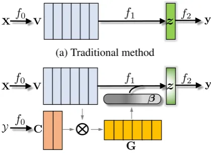
f =f0◦f1◦f2as shown in Figure1(a):

• f0:X7→V, the text sequence is represented

as its word-embedding form V, which is a

matrix ofP ×L.

• f1:V7→z, a compositional functionf1

ag-gregates word embeddings into a fixed-length

vector representationz.

• f2 :z 7→y, a classifierf2annotates the text

representationzwith a label.

A vast amount of work has been devoted to

de-vising the proper functions f0 and f1, i.e., how

to represent a word or a word sequence, respec-tively. The success of NLP largely depends on the

effectiveness of word embeddings in f0 (Bengio

et al.,2003;Collobert and Weston,2008;Mikolov

et al., 2013; Pennington et al., 2014). They are

often ptrained offline on large corpus, then

re-fined jointly via f1 and f2 for task-specific

rep-resentations. Furthermore, the design of f1 can

be broadly cast into two categories. The popu-lar deep learning models consider the mapping as a “black box,” and have employed sophisticated CNN/RNN architectures to achieve

state-of-the-art performance (Zhang et al.,2015;Yang et al.,

2016). On the contrary, recent studies show that

simple manipulation of the word embeddings,e.g.,

mean or max-pooling, can also provide

surpris-ingly excellent performance (Joulin et al., 2016;

Wieting et al.,2016;Arora et al.,2017;Shen et al.,

2018a). Nevertheless, these methods only lever-age the information from the input text sequence.

4 Label-Embedding Attentive Model

4.1 Model

By examining the three steps in the traditional pipeline of text classification, we note that the use of label information only occurs in the last step,

when learningf2, and its impact on learning the

representations of words inf0 or word sequences

inf1 is ignored or indirect. Hence, we propose a

new pipeline by incorporating label information in

(4)

V

<latexit sha1_base64="UZh7YjksYlFNc+xwF1GVx2T7SFE=">AAACCXicbVC7TsMwFHXKq5RXgJHFUCExVSlCArYKFsYikbZSE1WO47RWbSeyHVAVZWbhV1gYALHyB2z8DW6aAVqOZOn4nHvte0+QMKq043xblaXlldW16nptY3Nre8fe3euoOJWYuDhmsewFSBFGBXE11Yz0EkkQDxjpBuPrqd+9J1LRWNzpSUJ8joaCRhQjbaSBfegJ8oBjzpEIM6/Dkc6zzAsi2MnzWnEf2HWn4RSAi6RZkjoo0R7YX14Y45QToTFDSvWbTqL9DElNMSPm1VSRBOExGpK+oQJxovysWCWHx0YJYRRLc4SGhfq7I0NcqQkPTKWZbaTmvan4n9dPdXThZ1QkqSYCzz6KUgZ1DKe5wJBKgjWbGIKwpGZWiEdIIqxNejUTQnN+5UXinjYuG87tWb11VaZRBQfgCJyAJjgHLXAD2sAFGDyCZ/AK3qwn68V6tz5mpRWr7NkHf2B9/gAsmprB</latexit>

z

<latexit sha1_base64="5arKufyR9cN9ZiNsznhY2l36QxI=">AAACUnicbVJNTwIxEO3iFyIq6tFLIzHxRBZjot6IXjxiFCUBQrrdWaj2Y9N2MbDhPxoTD/4RLx60u3IQcJKmL++9aWemDWLOjPX9D6+wsrq2vlHcLG2Vt3d2K3v7D0YlmkKLKq50OyAGOJPQssxyaMcaiAg4PAbP15n+OAJtmJL3dhxDT5CBZBGjxDqqX3nqSnihSggiw7R7J4idpmk3iPDddFqa0wKwZJSLiodmLNyGc3LROFl0TTLHZNSvVP2anwdeBvUZqKJZNPuVt26oaCJAWsqJMZ26H9teSrRllIM7MzEQE/pMBtBxUBIBppfmM5niY8eEOFLaLWlxzv7NSIkwWX3O6ZoemkUtI//TOomNLnopk3FiQdLfi6KEY6twNmAcMg3U8rEDhGrmasV0SDSh1j1DyQ2hvtjyMmid1i5r/u1ZtXE1m0YRHaIjdILq6Bw10A1qohai6BV9om8Pee/eV8H9kl9rwZvlHKC5KJR/AHpCt3E=</latexit><latexit sha1_base64="5arKufyR9cN9ZiNsznhY2l36QxI=">AAACUnicbVJNTwIxEO3iFyIq6tFLIzHxRBZjot6IXjxiFCUBQrrdWaj2Y9N2MbDhPxoTD/4RLx60u3IQcJKmL++9aWemDWLOjPX9D6+wsrq2vlHcLG2Vt3d2K3v7D0YlmkKLKq50OyAGOJPQssxyaMcaiAg4PAbP15n+OAJtmJL3dhxDT5CBZBGjxDqqX3nqSnihSggiw7R7J4idpmk3iPDddFqa0wKwZJSLiodmLNyGc3LROFl0TTLHZNSvVP2anwdeBvUZqKJZNPuVt26oaCJAWsqJMZ26H9teSrRllIM7MzEQE/pMBtBxUBIBppfmM5niY8eEOFLaLWlxzv7NSIkwWX3O6ZoemkUtI//TOomNLnopk3FiQdLfi6KEY6twNmAcMg3U8rEDhGrmasV0SDSh1j1DyQ2hvtjyMmid1i5r/u1ZtXE1m0YRHaIjdILq6Bw10A1qohai6BV9om8Pee/eV8H9kl9rwZvlHKC5KJR/AHpCt3E=</latexit><latexit sha1_base64="5arKufyR9cN9ZiNsznhY2l36QxI=">AAACUnicbVJNTwIxEO3iFyIq6tFLIzHxRBZjot6IXjxiFCUBQrrdWaj2Y9N2MbDhPxoTD/4RLx60u3IQcJKmL++9aWemDWLOjPX9D6+wsrq2vlHcLG2Vt3d2K3v7D0YlmkKLKq50OyAGOJPQssxyaMcaiAg4PAbP15n+OAJtmJL3dhxDT5CBZBGjxDqqX3nqSnihSggiw7R7J4idpmk3iPDddFqa0wKwZJSLiodmLNyGc3LROFl0TTLHZNSvVP2anwdeBvUZqKJZNPuVt26oaCJAWsqJMZ26H9teSrRllIM7MzEQE/pMBtBxUBIBppfmM5niY8eEOFLaLWlxzv7NSIkwWX3O6ZoemkUtI//TOomNLnopk3FiQdLfi6KEY6twNmAcMg3U8rEDhGrmasV0SDSh1j1DyQ2hvtjyMmid1i5r/u1ZtXE1m0YRHaIjdILq6Bw10A1qohai6BV9om8Pee/eV8H9kl9rwZvlHKC5KJR/AHpCt3E=</latexit>

f

1

f0

X f2 y

(a) Traditional method

C

G

<latexit sha1_base64="usNIECuGP8YyDGtyIdesrnE+VfU=">AAACCXicbVC7TsMwFHV4lvIKMLIYKiSmKkVIwFbBUMYiEVqpiSrHcVqrthPZDqiKMrPwKywMgFj5Azb+BjfNAC1HsnR8zr32vSdIGFXacb6thcWl5ZXVylp1fWNza9ve2b1TcSoxcXHMYtkNkCKMCuJqqhnpJpIgHjDSCUZXE79zT6SisbjV44T4HA0EjShG2kh9+8AT5AHHnCMRZl6LI51nmRdEsJXn1eLet2tO3SkA50mjJDVQot23v7wwxiknQmOGlOo1nET7GZKaYkbMq6kiCcIjNCA9QwXiRPlZsUoOj4wSwiiW5ggNC/V3R4a4UmMemEoz21DNehPxP6+X6ujcz6hIUk0Enn4UpQzqGE5ygSGVBGs2NgRhSc2sEA+RRFib9KomhMbsyvPEPalf1J2b01rzskyjAvbBITgGDXAGmuAatIELMHgEz+AVvFlP1ov1bn1MSxessmcP/IH1+QPmwpqU</latexit>

<latexit sha1_base64="usNIECuGP8YyDGtyIdesrnE+VfU=">AAACCXicbVC7TsMwFHV4lvIKMLIYKiSmKkVIwFbBUMYiEVqpiSrHcVqrthPZDqiKMrPwKywMgFj5Azb+BjfNAC1HsnR8zr32vSdIGFXacb6thcWl5ZXVylp1fWNza9ve2b1TcSoxcXHMYtkNkCKMCuJqqhnpJpIgHjDSCUZXE79zT6SisbjV44T4HA0EjShG2kh9+8AT5AHHnCMRZl6LI51nmRdEsJXn1eLet2tO3SkA50mjJDVQot23v7wwxiknQmOGlOo1nET7GZKaYkbMq6kiCcIjNCA9QwXiRPlZsUoOj4wSwiiW5ggNC/V3R4a4UmMemEoz21DNehPxP6+X6ujcz6hIUk0Enn4UpQzqGE5ygSGVBGs2NgRhSc2sEA+RRFib9KomhMbsyvPEPalf1J2b01rzskyjAvbBITgGDXAGmuAatIELMHgEz+AVvFlP1ov1bn1MSxessmcP/IH1+QPmwpqU</latexit><latexit sha1_base64="usNIECuGP8YyDGtyIdesrnE+VfU=">AAACCXicbVC7TsMwFHV4lvIKMLIYKiSmKkVIwFbBUMYiEVqpiSrHcVqrthPZDqiKMrPwKywMgFj5Azb+BjfNAC1HsnR8zr32vSdIGFXacb6thcWl5ZXVylp1fWNza9ve2b1TcSoxcXHMYtkNkCKMCuJqqhnpJpIgHjDSCUZXE79zT6SisbjV44T4HA0EjShG2kh9+8AT5AHHnCMRZl6LI51nmRdEsJXn1eLet2tO3SkA50mjJDVQot23v7wwxiknQmOGlOo1nET7GZKaYkbMq6kiCcIjNCA9QwXiRPlZsUoOj4wSwiiW5ggNC/V3R4a4UmMemEoz21DNehPxP6+X6ujcz6hIUk0Enn4UpQzqGE5ygSGVBGs2NgRhSc2sEA+RRFib9KomhMbsyvPEPalf1J2b01rzskyjAvbBITgGDXAGmuAatIELMHgEz+AVvFlP1ov1bn1MSxessmcP/IH1+QPmwpqU</latexit>

z

<latexit sha1_base64="5arKufyR9cN9ZiNsznhY2l36QxI=">AAACUnicbVJNTwIxEO3iFyIq6tFLIzHxRBZjot6IXjxiFCUBQrrdWaj2Y9N2MbDhPxoTD/4RLx60u3IQcJKmL++9aWemDWLOjPX9D6+wsrq2vlHcLG2Vt3d2K3v7D0YlmkKLKq50OyAGOJPQssxyaMcaiAg4PAbP15n+OAJtmJL3dhxDT5CBZBGjxDqqX3nqSnihSggiw7R7J4idpmk3iPDddFqa0wKwZJSLiodmLNyGc3LROFl0TTLHZNSvVP2anwdeBvUZqKJZNPuVt26oaCJAWsqJMZ26H9teSrRllIM7MzEQE/pMBtBxUBIBppfmM5niY8eEOFLaLWlxzv7NSIkwWX3O6ZoemkUtI//TOomNLnopk3FiQdLfi6KEY6twNmAcMg3U8rEDhGrmasV0SDSh1j1DyQ2hvtjyMmid1i5r/u1ZtXE1m0YRHaIjdILq6Bw10A1qohai6BV9om8Pee/eV8H9kl9rwZvlHKC5KJR/AHpCt3E=</latexit><latexit sha1_base64="5arKufyR9cN9ZiNsznhY2l36QxI=">AAACUnicbVJNTwIxEO3iFyIq6tFLIzHxRBZjot6IXjxiFCUBQrrdWaj2Y9N2MbDhPxoTD/4RLx60u3IQcJKmL++9aWemDWLOjPX9D6+wsrq2vlHcLG2Vt3d2K3v7D0YlmkKLKq50OyAGOJPQssxyaMcaiAg4PAbP15n+OAJtmJL3dhxDT5CBZBGjxDqqX3nqSnihSggiw7R7J4idpmk3iPDddFqa0wKwZJSLiodmLNyGc3LROFl0TTLHZNSvVP2anwdeBvUZqKJZNPuVt26oaCJAWsqJMZ26H9teSrRllIM7MzEQE/pMBtBxUBIBppfmM5niY8eEOFLaLWlxzv7NSIkwWX3O6ZoemkUtI//TOomNLnopk3FiQdLfi6KEY6twNmAcMg3U8rEDhGrmasV0SDSh1j1DyQ2hvtjyMmid1i5r/u1ZtXE1m0YRHaIjdILq6Bw10A1qohai6BV9om8Pee/eV8H9kl9rwZvlHKC5KJR/AHpCt3E=</latexit>

<latexit sha1_base64="5arKufyR9cN9ZiNsznhY2l36QxI=">AAACUnicbVJNTwIxEO3iFyIq6tFLIzHxRBZjot6IXjxiFCUBQrrdWaj2Y9N2MbDhPxoTD/4RLx60u3IQcJKmL++9aWemDWLOjPX9D6+wsrq2vlHcLG2Vt3d2K3v7D0YlmkKLKq50OyAGOJPQssxyaMcaiAg4PAbP15n+OAJtmJL3dhxDT5CBZBGjxDqqX3nqSnihSggiw7R7J4idpmk3iPDddFqa0wKwZJSLiodmLNyGc3LROFl0TTLHZNSvVP2anwdeBvUZqKJZNPuVt26oaCJAWsqJMZ26H9teSrRllIM7MzEQE/pMBtBxUBIBppfmM5niY8eEOFLaLWlxzv7NSIkwWX3O6ZoemkUtI//TOomNLnopk3FiQdLfi6KEY6twNmAcMg3U8rEDhGrmasV0SDSh1j1DyQ2hvtjyMmid1i5r/u1ZtXE1m0YRHaIjdILq6Bw10A1qohai6BV9om8Pee/eV8H9kl9rwZvlHKC5KJR/AHpCt3E=</latexit>

<latexit sha1_base64="YJPS900Rs1XOpYUa1yiuV8LTbiU=">AAACM3icbVDLSgMxFM34rPVVdekmWARXZSqCuhPdCG4qdVRoS8lk7tRgHkOSUcrQj3Ljh7gRwYWKW//BzHQWVr0Qcjjn3uSeEyacGev7L97U9Mzs3Hxlobq4tLyyWltbvzQq1RQCqrjS1yExwJmEwDLL4TrRQETI4Sq8Pcn1qzvQhil5YYcJ9AQZSBYzSqyj+rWzroR7qoQgMsq6bUHsKMu6YYzbo1F1QgvBkrtCVDwyQ+EuXJB5YyH2a3W/4ReF/4JmCeqorFa/9tSNFE0FSEs5MabT9BPby4i2jHJwz6YGEkJvyQA6DkoiwPSywvQIbzsmwrHS7kiLC/bnREaEydd0nc7Vjfmt5eR/Wie18UEvYzJJLUg6/ihOObYK5wniiGmglg8dIFQztyumN0QTal3OVRdC87flvyDYbRw2/PO9+tFxmUYFbaIttIOaaB8doVPUQgGi6AE9ozf07j16r96H9zlunfLKmQ00Ud7XN5I5rWk=</latexit>

V

<latexit sha1_base64="UZh7YjksYlFNc+xwF1GVx2T7SFE=">AAACCXicbVC7TsMwFHXKq5RXgJHFUCExVSlCArYKFsYikbZSE1WO47RWbSeyHVAVZWbhV1gYALHyB2z8DW6aAVqOZOn4nHvte0+QMKq043xblaXlldW16nptY3Nre8fe3euoOJWYuDhmsewFSBFGBXE11Yz0EkkQDxjpBuPrqd+9J1LRWNzpSUJ8joaCRhQjbaSBfegJ8oBjzpEIM6/Dkc6zzAsi2MnzWnEf2HWn4RSAi6RZkjoo0R7YX14Y45QToTFDSvWbTqL9DElNMSPm1VSRBOExGpK+oQJxovysWCWHx0YJYRRLc4SGhfq7I0NcqQkPTKWZbaTmvan4n9dPdXThZ1QkqSYCzz6KUgZ1DKe5wJBKgjWbGIKwpGZWiEdIIqxNejUTQnN+5UXinjYuG87tWb11VaZRBQfgCJyAJjgHLXAD2sAFGDyCZ/AK3qwn68V6tz5mpRWr7NkHf2B9/gAsmprB</latexit>

f

0 X

Y

f

0

f2 _y

f

1

[image:4.595.77.287.62.216.2]

(b) Proposed joint embedding method

Figure 1: Illustration of different schemes for

doc-ument representationsz. (a) Much work in NLP

has been devoted to directly aggregating word

em-beddingV forz. (b) We focus on learning label

embeddingC(how to embed class labels in a

Eu-clidean space), and leveraging the “compatibility”

Gbetween embedded words and labels to derive

the attention scoreβfor improvedz. Note that_⊗

denotes the cosine similarity betweenCandV. In

this figure, there are K=2 classes.

• f0: Besides embedding words, we also

em-bed all the labels in the same space, which act as the “anchor points” of the classes to in-fluence the refinement of word embeddings.

• f1: The compositional function aggregates

word embeddings into z, weighted by the

compatibility between labels and words.

• f2: The learning off2remains the same, as it

directly interacts with labels.

Under the proposed label embedding framework, we specifically describe a label-embedding atten-tive model.

Joint Embeddings of Words and Labels We

propose to embed both the words and the labels

into a joint space i.e.,∆D _7→ RP andY 7→ RP.

The label embeddings are C = [c1,· · · ,cK],

whereKis the number of classes.

A simple way to measure the compatibility of label-word pairs is via the cosine similarity

G= (C>V)G,ˆ (2)

whereGˆ is the normalization matrix of sizeK_×L,

with each element obtained as the multiplication

of`2 norms of the c-th label embedding andl-th

word embedding:ˆgkl=kckkkvlk.

To further capture the relative spatial

informa-tion among consecutive words (i.e.,phrases1) and

introduce non-linearity in the compatibility mea-sure, we consider a generalization of (2).

Specif-ically, for a text phase of length 2r + 1

cen-tered at l, the local matrix block Gl−r:l+r in G

measures the label-to-token compatibility for the “label-phrase” pairs. To learn a higher-level

com-patibility stigmatizationulbetween thel-th phrase

and all labels, we have:

ul=ReLU(Gl−r:l+rW1+b1), (3)

whereW1 ∈R2r+1 andb1 ∈RK are parameters

to be learned, and ul ∈ RK. The largest

com-patibility value of thel-th phrasewrtthe labels is

collected:

ml=max-pooling(ul). (4)

Together,mis a vector of lengthL. The

compat-ibility/attention score for the entire text sequence is:

β=SoftMax(m), (5)

where the l-th element of SoftMax is βl =

exp(ml)

PL

l0=1exp(ml0)

.

The text sequence representation can be sim-ply obtained via averaging the word embeddings, weighted by label-based attention score:

z =X

l

βlvl. (6)

Relation to Predictive Text Embeddings

Pre-dictive Text Embeddings (PTE) (Tang et al.,2015)

is the first method to leverage label embeddings

to improve the learned word embeddings. We

discuss three major differences between PTE and

our LEAM:(i)The general settings are different.

PTE casts the text representation through hetero-geneous networks, while we consider text

repre-sentation through an attention model.(ii)In PTE,

the text representationz is the averaging of word

embeddings. In LEAM, z is weighted averaging

of word embeddings through the proposed

label-attentive score in (6).(iii)PTE only considers the

linear interaction between individual words and la-bels. LEAM greatly improves the performance by considering nonlinear interaction between phrase

1_{We call it “phrase” for convenience; it could be any}

longer word sequence such as a sentence and paragraphetc.

(5)

and labels. Specifically, we note that the text em-bedding in PTE is similar with a very special case

of LEAM, when our window sizer = 1 and

at-tention scoreβis uniform. As shown later in

Fig-ure2(c) of the experimental results, LEAM can be

significantly better than the PTE variant.

Training Objective The proposed joint

embed-ding framework is applicable to various text clas-sification tasks. We consider two setups in this paper. For a learned text sequence representation

z=f1◦f0(X), we jointly optimizef =f0◦f1◦f2

over_F, wheref2 is defined according to the

spe-cific tasks:

• Single-label problem: categorizes each text

instance to precisely one ofK classes,y _∈

∆K

min

f∈F

1 N

N

X

n=1

CE(yn, f2(zn)), (7)

where CE(_·,_·) is the cross entropy between

two probability vectors, and f2(zn) =

SoftMax(z0_n), with z0_n = W2zn +b2 and

W2 ∈RK×P,b2 ∈RKare trainable

param-eters.

• Multi-label problem: categorizes each text

instance to a set of K target labels {yk ∈

∆2_|k= 1,_{· · ·} , K_}; there is no constraint on

how many of the classes the instance can be assigned to, and

min

f∈F

1 N K

N

X

n=1

K

X

k=1

CE(ynk, f2(znk), (8)

wheref2(znk) = _1+exp(1_z0

nk), andz

0

nk is the

kth column ofz0_n.

To summarize, the model parameters θ =

{V,C,W1,b1,W2,b2}. They are trained

end-to-end during learning. {W1,b1} and{W2,b2}

are weights inf1 andf2, respectively, which are

treated as standard neural networks. For the joint

embeddings {V,C} in f0, the pre-trained word

embeddings are used as initialization if available.

4.2 Learning & Testing with LEAM

Learning and Regularization The quality of

the jointly learned embeddings are key to the

model performance and interpretability.

Ide-ally, we hope that each label embedding acts as

the “anchor” points for each classes: closer to the word/sequence representations that are in the same classes, while farther from those in different classes. To best achieve this property, we consider

to regularize the learned label embeddingsckto be

on its corresponding manifold. This is imposed by

the factckshould be easily classified as the correct

labelyk:

min

f∈F

1 K

K

X

n=1

CE(yk, f2(ck)), (9)

where f2 is specficied according to the problem

in either (7) or (8). This regularization is used as a penalty in the main training objective in (7) or (8), and the default weighting hyperparameter is set as 1. It will lead to meaningful interpretabil-ity of learned label embeddings as shown in the experiments.

Interestingly in text classification, the class

itself is often described as a set of E words

{ei, i = 1,· · · , E}. These words are

consid-ered as the most representative description of each class, and highly distinguishing between different

classes. For example, theYahoo!Answers Topic

dataset (Zhang et al., 2015) contains ten classes,

most of which have two words to precisely de-scribe its class-specific features, such as “Comput-ers & Internet”, “Business & Finance” as well as

“Politics & Government”etc. We consider to use

each label’s corresponding pre-trained word em-beddings as the initialization of the label embed-dings. For the datasets without representative class descriptions, one may initialize the label embed-dings as random samples drawn from a standard Gaussian distribution.

Testing Both the learned word and label

embed-dings are available in the testing stage. We

clar-ify that the label embeddingsCof all class

candi-dates_Y are considered as the input in the testing

stage; one should distinguish this from the use of

groundtruth label y in prediction. For a text

se-quence X, one may feed it through the proposed

pipeline for prediction:(i)f1: harvesting the word

embeddingsV,(ii)f2:Vinteracts withCto

ob-tainG, pooled as β, which further attendsV to

derive z, and (iii) f3: assigning labels based on

the tasks. To speed up testing, one may store G

(6)

Model Parameters Complexity Seq. Operation

CNN m·h·P O(m·h·L·P) O(1)

LSTM 4·h·(h+P) O(L·h2

+h·L·P) O(L)

SWEM 0 O(L·P) O(1)

Bi-BloSAN 7·P2+5·P O(P2·L2/R+P2·L+P2·R2) O(1)

[image:6.595.311.523.62.136.2]

Our model K·P O(K·L·P) O(1)

Table 1: Comparisons of CNN, LSTM, SWEM and our model architecture. Columns correspond to the number of compositional parameters, com-putational complexity and sequential operations

4.3 Model Complexity

We compare CNN, LSTM, Simple Word

Embeddings-based Models (SWEM) (Shen et al.,

2018a) and our LEAM wrt the parameters and

computational speed. For the CNN, we assume

the same size m for all filters. Specifically, h

represents the dimension of the hidden units in

the LSTM or the number of filters in the CNN;R

denotes the number of blocks in the Bi-BloSAN;

P denotes the final sequence representation

dimension. Similar to (Vaswani et al., 2017;

Shen et al., 2018a), we examine the number of

compositional parameters, computational com-plexity and sequential steps of the four methods.

As shown in Table 1, both the CNN and LSTM

have a large number of compositional parameters.

Since K m, h, the number of parameters in

our models is much smaller than for the CNN and LSTM models. For the computational complexity, our model is almost same order as the most simple SWEM model, and is smaller than the CNN or

LSTM by a factor ofmh/Korh/K.

5 Experimental Results

Setup We use 300-dimensional GloVe word

em-beddings Pennington et al. (2014) as

initializa-tion for word embeddings and label embeddings in our model. Out-Of-Vocabulary (OOV) words are initialized from a uniform distribution with

range[₋0.01,0.01]. The final classifier is

imple-mented as an MLP layer followed by a sigmoid or softmax function depending on specific task. We train our model’s parameters with the Adam

Optimizer (Kingma and Ba, 2014), with an

ini-tial learning rate of 0.001, and a minibatch size

of 100. Dropout regularization (Srivastava et al., 2014) is employed on the final MLP layer, with

dropout rate0.5. The model is implemented using

Tensorflow and is trained on GPU Titan X. The code to reproduce the experimental results

is at https://github.com/guoyinwang/LEAM

Dataset # Classes # Training # Testing

AGNews 4 120k 7.6k Yelp Binary 2 560 k 38k Yelp Full 5 650k 38k DBPedia 14 560k 70k Yahoo 10 1400k 60k

Table 2: Summary statistics of five datasets, in-cluding the number of classes, number of training samples and number of testing samples.

5.1 Classification on Benchmark Datasets

We test our model on the same five standard

benchmark datasets as in (Zhang et al.,2015). The

summary statistics of the data are shown in Table 2, with content specified below:

• AGNews: Topic classification over four cat-egories of Internet news articles (Del Corso

et al.,2005) composed of titles plus

descrip-tion classified into: World, Entertainment, Sports and Business.

• Yelp Review Full: The dataset is obtained from the Yelp Dataset Challenge in 2015, the task is sentiment classification of polarity star labels ranging from 1 to 5.

• Yelp Review Polarity: The same set of text reviews from Yelp Dataset Challenge in 2015, except that a coarser sentiment defini-tion is considered: 1 and 2 are negative, and 4 and 5 as positive.

• DBPedia: Ontology classification over four-teen non-overlapping classes picked from DBpedia 2014 (Wikipedia).

• Yahoo! Answers Topic: Topic classifica-tion over ten largest main categories from Ya-hoo! Answers Comprehensive Questions and Answers version 1.0, including question title, question content and best answer.

We compare with a variety of methods,

in-cluding (i) the bag-of-words in (Zhang et al.,

2015);(ii)sophisticated deep CNN/RNN models:

large/small word CNN, LSTM reported in (Zhang

et al.,2015;Dai and Le,2015) and deep CNN (29

layer) (Conneau et al.,2017);(iii)simple

compo-sitional methods: fastText (Joulin et al.,2016) and

simple word embedding models (SWEM) (Shen

et al., 2018a); (iv) deep attention models:

[image:6.595.73.291.62.113.2]

(7)

Model Yahoo DBPedia AGNews Yelp P. Yelp F.

Bag-of-words (Zhang et al.,2015) 68.90 96.60 88.80 92.20 58.00

Small word CNN (Zhang et al.,2015) 69.98 98.15 89.13 94.46 58.59

Large word CNN (Zhang et al.,2015) 70.94 98.28 91.45 95.11 59.48

LSTM (Zhang et al.,2015) 70.84 98.55 86.06 94.74 58.17

SA-LSTM (word-level) (Dai and Le,2015) - 98.60 - -

-Deep CNN (29 layer) (Conneau et al.,2017) 73.43 98.71 91.27 95.72 64.26

SWEM (Shen et al.,2018a) 73.53 98.42 92.24 93.76 61.11

fastText (Joulin et al.,2016) 72.30 98.60 92.50 95.70 63.90

HAN (Yang et al.,2016) 75.80 - - -

-Bi-BloSAN(Shen et al.,2018c) 76.28 98.77 93.32 94.56 62.13

LEAM 77.42 99.02 92.45 95.31 64.09

[image:7.595.74.522.61.240.2]

LEAM (linear) 75.22 98.32 91.75 93.43 61.03

Table 3: Test Accuracy on document classification tasks, in percentage. We ran Bi-BloSAN using the

authors’ implementation; all other results are directly cited from the respective papers.

2016);(v)simple attention models: bi-directional

block self-attention network (Bi-BloSAN) (Shen

et al.,2018c). The results are shown in Table3.

Testing accuracy Simple compositional

meth-ods indeed achieve comparable performance as the

sophisticated deep CNN/RNN models. On the

other hand, deep hierarchical attention model can improve the pure CNN/RNN models. The recently proposed self-attention network generally yield higher accuracy than previous methods. All ap-proaches are better than traditional bag-of-words method. Our proposed LEAM outperforms the state-of-the-art methods on two largest datasets,

i.e., Yahoo and DBPedia. On other datasets,

LEAM ranks the 2nd or 3rd best, which are simi-lar to top 1 method in term of the accuracy. This

is probably due to two reasons: (i) the number

of classes on these datasets is smaller, and (ii)

there is no explicit corresponding word embed-ding available for the label embedembed-ding initializa-tion during learning. The potential of label embed-ding may not be fully exploited. As the ablation study, we replace the nonlinear compatibility (3) to the linear one in (2) . The degraded performance demonstrates the necessity of spatial dependency and nonlinearity in constructing the attentions.

Nevertheless, we argue LEAM is favorable for text classification, by comparing the model size

and time cost Table 4, as well as convergence

speed in Figure 2(a). The time cost is reported

as the wall-clock time for 1000 iterations. LEAM maintains the simplicity and low cost of SWEM, compared with other models. LEAM uses much less model parameters, and converges significantly

Model # Parameters Time cost (s)

CNN 541k 171 LSTM 1.8M 598

SWEM 61K 63

Bi-BloSAN 3.6M 292

LEAM 65K 65

Table 4: Comparison of model size and speed.

faster than Bi-BloSAN. We also compare the per-formance when only a partial dataset is labeled,

the results are shown in Figure2(b). LEAM

con-sistently outperforms other methods with different proportion of labeled data.

Hyper-parameter Our method has an

addi-tional hyperparameter, the window sizerto define

the length of “phase” to construct the attention.

Larger r captures long term dependency, while

smallerrenforces the local dependency. We study

its impact in Figure2(c). The topic classification

tasks generally requires a larger r, while

senti-ment classification tasks allows relatively smaller

r. One may safely chooseraround50if not

fine-tuning. We report the optimal results in Table3.

5.2 Representational Ability

Label embeddings are highly meaningful To

provide insight into the meaningfulness of the

learned representations, in Figure 3 we

visual-ize the correlation between label embeddings and document embeddings based on the Yahoo date-set. First, we compute the averaged document

em-beddings per class:zk¯ = _|S1

k| P

i∈Skzi, whereSk

is the set of sample indices belonging to classk.

[image:7.595.320.510.290.369.2]

(8)

0 2K 4K

# Iteration

50 60 70 80

Accuracy (%) _LEAM

CNN LSTM Bi-Blosa

0.1 1 10 100

Proportion (%) of labeled data

40 60 80

Accuracy (%) _LEAM

CNN LSTM SWEM

76.0 76.5 77.0

Yahoo!

98.6 98.8 99.0

DBPedia

0 25 50 75 94.0

94.5 95.0

Yelp Polarity

0 25 50 75

# Window Size

61 62 63 64

Accuracy (%)

Yelp Full

[image:8.595.83.528.63.197.2]

(a) Convergence speed (b) Partially labeled data (c) Effects of window size

Figure 2: Comprehensive study of LEAM, including convergence speed, performance vs proportion of labeled data, and impact of hyper-parameter

0.1 0.0 0.1 0.2 0.3 0.4

Society Culture Science Mathematics Health

Education Reference Computers Internet Sports

Business Finance Entertainment Music Family Relationships Politics Government

(a) Cosine similarity matrix (b) t-SNE plot of joint embeddings

Figure 3: Correlation between the learned text sequence representationz and label embedding V. (a)

Cosine similarity matrix between averagedz¯per class and label embeddingV, and (b) t-SNE plot of

joint embedding of textzand labelsV.

text manifold for classk. Ideally, the perfect label

embeddingckshould be the representative anchor

point for classk. We compute the cosine

similar-ity betweenz¯kandckacross all the classes, shown

in Figure 3(a). The rows are averaged per-class

document embeddings, while columns are label embeddings. Therefore, the on-diagonal elements measure how representative the learned label em-beddings are to describe its own classes, while off-diagonal elements reflect how distinctive the label embeddings are to be separated from other classes. The high on-diagonal elements and low

off-diagonal elements in Figure 3(a) indicate the

superb ability of the label representations learned from LEAM.

Further, since both the document and label em-beddings live in the same high-dimensional space,

we use t-SNE (Maaten and Hinton, 2008) to

vi-sualize them on a 2D map in Figure 3(b). Each

color represents a different class, the point clouds are document embeddings, and the label embed-dings are the large dots with black circles. As can be seen, each label embedding falls into the

inter-nal region of the respective manifold, which again demonstrate the strong representative power of la-bel embeddings.

Interpretability of attention Our attention

scoreβ can be used to highlight the most

infor-mative wordswrtthe downstream prediction task.

We visualize two examples in Figure4(a) for the

Yahoo dataset. The darker yellow means more im-portant words. The 1st text sequence is on the topic of “Sports”, and the 2nd text sequence is “Entertainment”. The attention score can correctly detect the key words with proper scores.

5.3 Applications to Clinical Text

To demonstrate the practical value of label embed-dings, we apply LEAM for a real health care sce-nario: medical code prediction on the Electronic Health Records dataset. A given patient may have multiple diagnoses, and thus multi-label learning is required.

Specifically, we consider an open-access

[image:8.595.81.520.248.388.2]

(9)

AUC F1

Model Macro Micro Macro Micro P@5

Logistic Regression 0.829 0.864 0.477 0.533 0.546

Bi-GRU 0.828 0.868 0.484 0.549 0.591

CNN (Kim,2014) 0.876 0.907 0.576 0.625 0.620

C-MemNN (Prakash et al.,2017) 0.833 - - - 0.42

Attentive LSTM (Shi et al.,2017) - 0.900 - 0.532

-CAML (Mullenbach et al.,2018) 0.875 0.909 0.532 0.614 0.609

[image:9.595.122.479.60.189.2]

LEAM 0.881 0.912 0.540 0.619 0.612

Table 5: Quantitative results for doctor-notes multi-label classification task.

contains text and structured records from a hospital intensive care unit. Each record includes a variety of narrative notes describing a patients stay, including diagnoses and procedures. They are accompanied by a set of metadata codes from the International Classification of Diseases (ICD), which present a standardized way of indicating diagnoses/procedures. To compare with previous

work, we follow (Shi et al., 2017; Mullenbach

et al., 2018), and preprocess a dataset consisting

of the most common 50 labels. It results in 8,067 documents for training, 1,574 for validation, and 1,730 for testing.

Results We compare against the three

base-lines: a logistic regression model with bag-of-words, a bidirectional gated recurrent unit (Bi-GRU) and a single-layer 1D convolutional

net-work (Kim, 2014). We also compare with three

recent methods for multi-label classification of clinical text, including Condensed Memory

Net-works (C-MemNN) (Prakash et al.,2017),

Atten-tive LSTM (Shi et al., 2017) and Convolutional

Attention (CAML) (Mullenbach et al.,2018).

To quantify the prediction performance, we

fol-low (Mullenbach et al., 2018) to consider the

micro-averaged and macro-averaged F1 and area under the ROC curve (AUC), as well as the

preci-sion atn(P@n). Micro-averaged values are

cal-culated by treating each (text, code) pair as a sep-arate prediction. Macro-averaged values are cal-culated by averaging metrics computed per-label.

P@nis the fraction of thenhighestscored labels

that are present in the ground truth.

The results are shown in Table5. LEAM

pro-vides the best AUC score, and better F1 and P@5 values than all methods except CNN. CNN con-sistently outperforms the basic Bi-GRU architec-ture, and the logistic regression baseline performs worse than all deep learning architectures.

(a) Yahoo dataset

(b) Clinical text

Figure 4: Visualization of learned attentionβ.

We emphasize that the learned attention can be very useful to reduce a doctor’s reading burden.

As shown in Figure4(b), the health related words

are highlighted.

6 Conclusions

In this work, we first investigate label embed-dings for text representations, and propose the label-embedding attentive models. It embeds the words and labels in the same joint space, and mea-sures the compatibility of word-label pairs to

at-tend the document representations. The

learn-ing framework is tested on several large standard datasets and a real clinical text application. Com-pared with the previous methods, our LEAM al-gorithm requires much lower computational cost, and achieves better if not comparable performance relative to the state-of-the-art. The learned atten-tion is highly interpretable: highlighting the most informative words in the text sequence for the downstream classification task.

Acknowledgments This research was supported

(10)

References

Zeynep Akata, Florent Perronnin, Zaid Harchaoui, and Cordelia Schmid. 2016. Label-embedding for image classification. IEEE transactions on pattern analy-sis and machine intelligence.

Sanjeev Arora, Yingyu Liang, and Tengyu Ma. 2017. A simple but tough-to-beat baseline for sentence em-beddings.ICLR.

Dzmitry Bahdanau, Kyunghyun Cho, and Yoshua Ben-gio. 2015. Neural machine translation by jointly learning to align and translate. ICLR.

Yoshua Bengio, R´ejean Ducharme, Pascal Vincent, and Christian Jauvin. 2003. A neural probabilistic lan-guage model. Journal of machine learning research.

Ronan Collobert and Jason Weston. 2008. A unified architecture for natural language processing: Deep neural networks with multitask learning. In Pro-ceedings of the 25th international conference on Machine learning.

Alexis Conneau, Holger Schwenk, Lo¨ıc Barrault, and Yann Lecun. 2017. Very deep convolutional net-works for text classification. InProceedings of the 15th Conference of the European Chapter of the As-sociation for Computational Linguistics: Volume 1, Long Papers, volume 1, pages 1107–1116.

Yiming Cui, Zhipeng Chen, Si Wei, Shijin Wang, Ting Liu, and Guoping Hu. 2016. Attention-over-attention neural networks for reading comprehen-sion.arXiv preprint arXiv:1607.04423.

Andrew M Dai and Quoc V Le. 2015. Semi-supervised sequence learning. InAdvances in Neural Informa-tion Processing Systems, pages 3079–3087.

Gianna M Del Corso, Antonio Gulli, and Francesco Romani. 2005. Ranking a stream of news. In

Proceedings of the 14th international conference on World Wide Web. ACM.

Andrea Frome, Greg S Corrado, Jon Shlens, Samy Bengio, Jeff Dean, Tomas Mikolov, et al. 2013. De-vise: A deep visual-semantic embedding model. In

NIPS.

Jonas Gehring, Michael Auli, David Grangier, De-nis Yarats, and Yann N Dauphin. 2017. Convolu-tional sequence to sequence learning. arXiv preprint arXiv:1705.03122.

Sepp Hochreiter and J¨urgen Schmidhuber. 1997. Long short-term memory.Neural computation.

Alistair EW Johnson, Tom J Pollard, Lu Shen, H Lehman Li-wei, Mengling Feng, Moham-mad Ghassemi, Benjamin Moody, Peter Szolovits, Leo Anthony Celi, and Roger G Mark. 2016. Mimic-iii, a freely accessible critical care database.

Scientific data.

Armand Joulin, Edouard Grave, Piotr Bojanowski, and Tomas Mikolov. 2016. Bag of tricks for efficient text classification.EACL.

Nal Kalchbrenner, Edward Grefenstette, and Phil Blun-som. 2014. A convolutional neural network for modelling sentences. ACL.

Yoon Kim. 2014. Convolutional neural net-works for sentence classification. arXiv preprint arXiv:1408.5882.

Diederik P Kingma and Jimmy Ba. 2014. Adam: A method for stochastic optimization. arXiv preprint arXiv:1412.6980.

Ryan Kiros, Ruslan Salakhutdinov, and Richard S Zemel. 2014. Unifying visual-semantic embeddings with multimodal neural language models. NIPS 2014 deep learning workshop.

Ryan Kiros, Yukun Zhu, Ruslan R Salakhutdinov, Richard Zemel, Raquel Urtasun, Antonio Torralba, and Sanja Fidler. 2015. Skip-thought vectors. In

Advances in neural information processing systems.

Quoc Le and Tomas Mikolov. 2014. Distributed rep-resentations of sentences and documents. In Inter-national Conference on Machine Learning, pages 1188–1196.

Chunyuan Li, Heerad Farkhoor, Rosanne Liu, and Ja-son Yosinski. 2018. Measuring the intrinsic dimen-sion of objective landscapes. InInternational Con-ference on Learning Representations.

Yukun Ma, Erik Cambria, and Sa Gao. 2016. Label embedding for zero-shot fine-grained named entity typing. InCOLING.

Laurens van der Maaten and Geoffrey Hinton. 2008. Visualizing data using t-sne. Journal of machine learning research.

Tomas Mikolov, Ilya Sutskever, Kai Chen, Greg S Cor-rado, and Jeff Dean. 2013. Distributed representa-tions of words and phrases and their compositional-ity. InAdvances in neural information processing systems, pages 3111–3119.

James Mullenbach, Sarah Wiegreffe, Jon Duke, Jimeng Sun, and Jacob Eisenstein. 2018. Explainable pre-diction of medical codes from clinical text. arXiv preprint arXiv:1802.05695.

Mark Palatucci, Dean Pomerleau, Geoffrey E Hinton, and Tom M Mitchell. 2009. Zero-shot learning with semantic output codes. InNIPS.

(11)

Aaditya Prakash, Siyuan Zhao, Sadid A Hasan, Vivek V Datla, Kathy Lee, Ashequl Qadir, Joey Liu, and Oladimeji Farri. 2017. Condensed memory net-works for clinical diagnostic inferencing. InAAAI.

Jose A Rodriguez-Serrano, Florent Perronnin, and France Meylan. 2013. Label embedding for text recognition. InProceedings of the British Machine Vision Conference.

Alexander M Rush, Sumit Chopra, and Jason We-ston. 2015. A neural attention model for ab-stractive sentence summarization. arXiv preprint arXiv:1509.00685.

Dinghan Shen, Guoyin Wang, Wenlin Wang, Martin Renqiang Min, Qinliang Su, Yizhe Zhang, Chun-yuan Li, Ricardo Henao, and Lawrence Carin. 2018a. Baseline needs more love: On simple word-embedding-based models and associated pool-ing mechanisms. InACL.

Dinghan Shen, Yizhe Zhang, Ricardo Henao, Qinliang Su, and Lawrence Carin. 2017. Deconvolutional latent-variable model for text sequence matching.

AAAI.

Tao Shen, Tianyi Zhou, Guodong Long, Jing Jiang, Shirui Pan, and Chengqi Zhang. 2018b. Disan: Di-rectional self-attention network for rnn/cnn-free lan-guage understanding. AAAI.

Tao Shen, Tianyi Zhou, Guodong Long, Jing Jiang, and Chengqi Zhang. 2018c. Bi-directional block self-attention for fast and memory-efficient sequence modeling. ICLR.

Haoran Shi, Pengtao Xie, Zhiting Hu, Ming Zhang, and Eric P Xing. 2017. Towards automated icd coding using deep learning. arXiv preprint arXiv:1711.04075.

Nitish Srivastava, Geoffrey Hinton, Alex Krizhevsky, Ilya Sutskever, and Ruslan Salakhutdinov. 2014. Dropout: A simple way to prevent neural networks from overfitting. The Journal of Machine Learning Research.

Jian Tang, Meng Qu, and Qiaozhu Mei. 2015. Pte: Pre-dictive text embedding through large-scale hetero-geneous text networks. InProceedings of the 21th ACM SIGKDD International Conference on Knowl-edge Discovery and Data Mining, pages 1165–1174. ACM.

Ashish Vaswani, Noam Shazeer, Niki Parmar, Jakob Uszkoreit, Llion Jones, Aidan N Gomez, Łukasz Kaiser, and Illia Polosukhin. 2017. Attention is all you need. InAdvances in Neural Information Pro-cessing Systems, pages 6000–6010.

Sida Wang and Christopher D Manning. 2012. Base-lines and bigrams: Simple, good sentiment and topic classification. InACL.

Wenlin Wang, Zhe Gan, Wenqi Wang, Dinghan Shen, Jiaji Huang, Wei Ping, Sanjeev Satheesh, and Lawrence Carin. 2018. Topic compositional neural language model.AISTATS.

John Wieting, Mohit Bansal, Kevin Gimpel, and Karen Livescu. 2016. Towards universal paraphrastic sen-tence embeddings. ICLR.

Zichao Yang, Diyi Yang, Chris Dyer, Xiaodong He, Alex Smola, and Eduard Hovy. 2016. Hierarchi-cal attention networks for document classification. In North American Chapter of the Association for Computational Linguistics: Human Language Tech-nologies.

Wenpeng Yin, Hinrich Sch¨utze, Bing Xiang, and Bowen Zhou. 2016. Abcnn: Attention-based convo-lutional neural network for modeling sentence pairs.

TACL.

Dani Yogatama, Daniel Gillick, and Nevena Lazic. 2015. Embedding methods for fine grained entity type classification. InACL.

Honglun Zhang, Liqiang Xiao, Wenqing Chen, Yongkun Wang, and Yaohui Jin. 2017a. Multi-task label embedding for text classification. arXiv preprint arXiv:1710.07210.

Xiang Zhang, Junbo Zhao, and Yann LeCun. 2015. Character-level convolutional networks for text clas-sification. InNIPS.

Yizhe Zhang, Dinghan Shen, Guoyin Wang, Zhe Gan, Ricardo Henao, and Lawrence Carin. 2017b. De-convolutional paragraph representation learning. In

NIPS.