Some Approximation in Cone Metric Space and Variational Iterative Method

http://dx.doi.org/10.4236/am.2012.312276 Published Online December 2012 (http://www.SciRP.org/journal/am)

Some Approximation in Cone Metric Space and

Variational Iterative Method

Ning Chen, Jiqian Chen

School of Science, Southwest University of Science and Technology, Mianyang, China Email: [email protected], [email protected]

Received September 23, 2012; revised October 23, 2012; accepted November 1, 2012

ABSTRACT

In this paper, we give some new results of common fixed point theorems and coincidence point case for some iterative method. By using of variation iteration method and an effective modification of He’s variation iteration method dis- cusses some integral and differential equations, we give out some new conclusion and more new examples.

Keywords: Cone Metric Space; Common Fixed Point; Effective Variation Iteration Method; Integral-Differential Equation

1. Introduction

Fixed point theory has fascinated many researchers since 1922 with the celebrated Banach’s fixed point theorem. There exist a fast literature on the topic and this is a very active field of research at present (See [1-7]).

By using same definition and meaning in stating is also looking in [2] and [3] etc. we introducing the fol- lowing results for needing. For convenience, the authors give the following definition and lemma (see the proof of theorem 3 [2])

Let always be a real Banach space, and be the subset of is called a cone, if and only if:

E P

, E P

(i) P is closed, nonempty, and

a

 

0 ;

P

ax by P

 

(ii) ,bR a b, , 0, ,x yP 

, and 0.

xP    x P x

;

(iii)

Given a conePE,we define a partial ordering  with respect to P by x y if and only if y x P.

We shall write xy to indicate x y but x y while xy

P

implies int denotes the interior of .

int ,

y x P P

Definition 1.1 Let X be a non-empty set in , and suppose the mapping satisfies:

E :

d X X E (i) 0d x y



,



for any x y, X, and

 

,y  0 x

 

,

d x y d

;



,

d x y



y

(ii) x for all x y, X;



,y

(iii) d x y

 

, d x z



,



d z



for all x y z, , X.

Then d is cone distance on X,



X d,



is called a cone metric space.

It is obvious that cone metric space generalize the metric spaces.

Definition 1.2 Let



X d,



is said to be a complete cone metric space, if every Cauchy sequence is con-

vergent in X.

Let



X d,



be a metric space. We denote by CB X

 

.

the family of non-empty closed bounded subset of X

Let H

 

 , be the Hausdorff metric on CB

 

X . That is for



,



max sup





,



, sup



,





a A b B

.

H A B d a B d A b

 



where



,



inf



d a b b

 

, , B



.

B

d a B

a

 is the distance from point to the sub-set An element xX is said to be a fixed point of a multi-valued mapping

 

: 2 ifX .

T X  x T X



,



Lemma 1.3 Suppose that X d be a cone metric space and the mapping T X: X hold the sequence

 

xn in



X d,



satisfying the following conditions:



n1,xn



Ld x x



n, n1

 

, 0L



d x 1 ,

and that is



1,





1,

n

n n

d x_ x L d x x₀



.

Then the sequence

 

xn is a Cauchy sequence in



X d,



.

integral equations.

Such theorems are very important tools for proving the existence and eventually the uniqueness of the solutions to various mathematical models (integral and partial dif- ferential equations, variations inequalities etc.).

[image:2.595.328.516.86.211.2]

First, we state following some extend conclusion ([3, 4]). Next, authors consider the variation iterative method to some integral and differential equations, and effective method ([5-8]) for examples and numerical test as some Fig case.

Now we first give common fixed point Theorem in similar method for two operators to extend Theorem 2.1 [2] with one operator case. Assume that



X d,



be a complete cone metric space.

Theorem 2.1 Let



X d,



be a complete cone metric space, P a normal cone with normal constant K.

Suppose that mappings satisfies the Con- tractive condition

, :

S T X X









 













 

2

, ,

,

,

1 ,

d Sx Ty k d Sx x d Ty y

d x Ty

d x y

d x Ty



 

 

,

,

(2.1)

for each x y, X where k



0,1 2



is a constant Then has a unique common fixed point in



0  2 ,



.

, S T

X And so for any xX, the iterative se- quence

 

n con- verges to the fixed point.

T x

Corollary 2.2 Let  0, and T then we obtain that theorem 2.1 in [2].

S 

In the same way, authors can extend theorem 4 [2], and omit again these stating.

3. Some Notes of Common Fixed Point

The common fixed point theorems for two operators in cone metric space are given in [3]. By using of needing same definition and as same results in it, we consider fixed point theorem in cone metric space to complete and extending the Theorem 1 in it.

Theorem A (See Theorem 1 [3]) Assume that



X d,



be a complete cone metric space. Let mappings

satisfying following Lipchitz conditions for any

, : S T X X

, ,

x yX





   

  



  



  



  



, , ,

, , , ,

, , , ,

d Sx Ty A x y d x y

B x y d x Sx C x y d y Ty

D x y d x Ty E x y d y Sx



 

  ,

(3.0)

where A B C D E F, , , , , ,

are nonnegative real value func- tions on XX such that





























,

, , , 1, ,

1, , , 1

A x y D x y E x y C x y D x y B x y E x y



  

  

,

and that

 

 

 

 

 

 

 

 

 

 

 

 

 

 

 

 

 

 

1 ,

2 ,

3 ,

4 2

,

, , ,

sup ,

1 , ,

, , ,

sup ,

1 , ,

1 , ,

sup ,

1 , ,

1 , ,

sup 1.

1 , , ,

x y X

x y X

x y X

x y X

A x y B x y D x y L

C x y D x y

A x y C x y E x y L

B x y E x y

C x y D x y B x y E x y

B x y E x y

L K

C x y D x y

L









 



 

 



 

 



 

 

2 L L

  

 

Then there is a unique common fixed point in uX

for S and T, and for any x0X, the iterative se- quence

 

xn convergent to the common fixed point of

,

S T



x2k1Sx2k,x2k2Tx2k1,k0,1,2,



.

Remark in [3], the example 2 illustrate this effect of meanings with this Theorem (non-expansion mapping, not contractive case that have uniqueness common fixed point). Look for multiple-value mappings in some case [5].

We can easy note Theorem A. Now we give complete this fixed point problem below.

Theorem 3.1 Same as the assume of theorem 1 [3]. Let



X d,



, ,

be a complete cone metric space, and there exists positive integer and mappings

satisfying following Lipchitz conditions for any

,

p q S T X, : X

x yX that is satisfy following inequality such that





   

 





 



 





 





, , ,

, , , ,

, , , ,

p q

p q

q p

d S x T y A x y d x y

B x y d x S x C x y d y T y



, D x y d x T y E x y d y S x



 

 

(3.1)

where A B C D E, , , , .

are non-negative real functions on

XX If it holds, STTS.

Then there is a unique common fixed point in uX

for SandT.

Proof By the proof of theorem 1 [3] that we known that Sp and has a unique common fixed point and

q

T u,

 

 

,

Sp u Tq u u from

 

 

, q

 

 

q ,

Sp Tu T S up Tu T u T T u Tu

then Tu is also common fixed point of Sp and Hence, we have

q

T Tuu by the uniqueness of them. In the same way, we know that Suu. that is, Suu. This u is a common fixed point of SandT, and

 

 

,

 

 

p p q q

S Su S S u Su T Tu uT T u Tu

We have SuTuu.

On the other hand, if SvTvv v



u



, then clearly, ,

p q

theorem.

Theorem 3.2 Let



X d,



, i: S T

be a complete cone metric space, and mappings sat- isfying following Lipchitz conditions for any



1, 2, ,



X X i  m

, ,

x yX

that is satisfy following inequality ( , , , ,A B C D E non- negative real constant)

























, , ,

, , for any , ,

i i

i

d Sx T y Ad x y Bd x Sx Cd y T y

Dd x T y Ed y Sx x y X

  

  

,

(3.2)

and



,



1, , , or C B E D .

A    B C D E CB ED  

If 1 2 have not common fixed point each other, then the exist at least number fixed points in

, , , m

T T T

S

.

m

X

Proof By the theorem 1 [3], we known that and has a unique common fixed point that is

and that in the same way,

S

i T S u

,

i u

 

1 T u1

 

1 u1,

 

2 2

 

2 2, ,

 

m m

 

m m.

S u T u u  S u T u u

Then S have at least m number fixed points.

Corollary 3.3 Let more positive integer cases in theorem 3.1.

1,

q p

Remark 3.4 (see corollary 5 [3]) Assume that



X d,



, ,

be complete cone metric space, and mappings satisfy following condition (

, :

S T X X A B C D E, ,

non-negative real constant):





 















, , ,

, , for any ,

d Sx Ty Ad x y Bd x Sx Cd y Ty

Dd x Ty Ed y Sx x y X

  

  



,

, (3.3) And





,

1, , or, , ,

A B C    D E CB ED CB E D

then must have uniqueness common fixed point, and for any 0

, S T

,

x X iterative sequence

 

xn conver-

gent to the common fixed point



x2k1Sx2k,x2k2 Tx2k1,k0,1,2,



.



Here example 2 in [5] for non-expansion mappings, also have common fixed point case with important mean- ings.

4. Common Fixed Point of Four Mappings

Many authors have extended the contraction mapping principle in difference direction. Some extension of Ba- nach’s fixed point theorem through the rational expres- sion form with it’s inequality. The purpose of this section, is to establish some common fixed point theorem for four mappings in this space.

Theorem 4.1 Assume that



X d,

S T

be a complete cone metric space, and mappings

continuous and satisfying following conditions for any

, , ,E F X: X

 

   

 

, : , ,

, ,

x y X ES SE FT TF

E X T X F X S X

  

 

and that inequality















 

 

 







,

, ,

,

, , ,

, ,

for any , , and , ,

0, 0 1

d Ex Ty

d Sx Ex d Ty Ex

d Tx Fy

d Sx Fy d Ty Ex d Sx Ty

d Sx Ty

x y X Sx Ty

 



 

   

 

 



 

    

(4.1)

Then have a unique common fixed point.

, , and

E F S T

Proof Let x0 be an arbitrary point of Xand from

 

 

,

E X T X we can choose a pointx1Xsuch that

1 0.

Tx Ex Also F X

 

S X





, we can choose a point x2X such that In general, we can Choose

2 .

Sx Sx₁

2n1

x _ X and x2n2X define a sequence

 

xn in X. as follows,

2 1 2 2

2 2 2 1 2 1 .

,

, 0,1, 2,

n n n

n n n

Tx Ex y

Sx Fx y n



  

 

   

Now, by (4.1) we have that



















 

 























2 1 2 2

2 2 1 2 2 1 2 2

2 2 1 2 2 1 2 2 1

2 1 2

2 1 2

2 1 2

,

, ,

,

,

, ,

,

.

,

,

n n

n n n n

n n

n n

n n n n

n n

n n

n n

d Tx Sx

d Ex Fx d y y

d Sx Ex

d y y

d Sx Fx Sx Tx

d y y

d

d

y y

y y



     

 

 



 







 



 

 

  

Similarly, we have











2 12 22 2 2 1

 

2 1 2 2





2 2 1



, ,

, , .

n n n n

n n n n

d y y d Fx Ex

d Ex Fx    d y y

   

  



   

which implies that



n 1, n 2









n 1, n



, 0,1, 2, .

d y _ y _      d y _ y n 

Hence, it is well know that

 

yn is Cauchy sequence.

From the X. is complete, then there exists uX

such that the

 

yn convergences to u in X. Since



Ex2n



and



Fx2n1



are subsequences of

 

yn then it

will convergence to same point u.

Next, from these are continuous maps, we can obtain following results

, , and

E F S T



2n



and



2n 1







.

E Sx Eu F Tx _ Fu n 

It follows from ESSEandFT TF, then we have



_2n





_2n



Eu, Su

By (4.1), if EuFu, then same reason,













, ,

, ,

d Eu Fu d Su Tu

d Eu Fu 



   

 







2n 1





2n 1







,

T Fx _ F Tx _ Fu n 



, ,

we again obtain TuFu. By (4.1), if SuTu, then



,





,





d Eu Fu d Su Tu d Eu Fu

also a contradiction. Thus, we have this is a contradiction. Hence, we have that _Su_Eu_Fu_Tu_u_,

u



SuEuFuTu

Let SuEuFuTuu, then we obtain that

 

 

 

,

EuE Eu E Su S Eu Su

then this implies u for common fixed point of .

E

_ , , and

E F S T

(Uniqueness) Let two points be the difference common fixed point of



.

,

u u uu

, , and

E F S T

and

 

 

 

.

FuF Tu T Fu T Eu Tu By (4.1), we have



 









, ,

, ,

d u u d Eu Fu

d Su Tu d u u

 

   



.    



 

By (4.1), if Fuu, then



 









, ,

, ,

d u Fu d Eu Fu

d Su Tu d u Fu

 

  

 



  



, _{A contradiction in the above same reason, then this}

implies the uniqueness of common fixed point of .

, , and

E F S T

we get  1.

It is a contradiction. Thus, FuTuu.

Remarks Similarly,

(i) As  0,S T, we obtain special case.



 









, ,

, ,

d Su u d Eu Fu

d Su Tu d Su u

 

   

   



 

(ii) S  T I (Identity map), EF, 0, we get some special case.



,

Theorem 4.2 Assume that



X d,



be a complete cone metric space. Same as theorem 4.1, and satisfies these conditions below

we get  1.

It is also a contradiction. Therefore, SuEuu.

 

 

 

 

, , and and

ES SE FTTF E X T X F X S X



,







,

 







,









,







1 , , ,

p p

p q q

q p

d Sx E x d Ty E x

d E x T y d Tx F y d Sx Ty

d Sx F y d Ty E x d Sx Ty

 

 

 

   , ,

1

Let : 0,



 





0,



be a strictly increasing func-tion such that

for any

, , and , , 0, 0

x yX SxTy           (4.2)

(i) 

 

0 0,

Then have a unique common fixed point.

, , and

E F S T

(ii) 0

 

t tfor each t0, Proof By theorem 4.1, we known that there is a unique

fixed point u in X, and _{SuE u}p _{F u}q _Tuu. .

Fu Tuu

(iii)

 

1

n i

t  



 



for each t



0,



.

Obviously, This completes the proof of theorem 4.2.

SuEu 

Now, we can easy obtain following theorems.

Theorem 5.1 Let



X d,



be a complete metric space and S T, _i:X CB

 

X be multi-valued maps

5. Some Notes for Multi-Valued Mappings



_{i1, 2,,m}



satisfying for each x y, X,

According the direction of [5], we give out some coinci-dence point theorem of maps to extend theorem 2.1 and theorem 2.3 [5].



, _i



max



, , , _i



,

H Sx T y    x y Sx T y

where

 



d x y d x Sx d y T y

  

, , ,

 

, , i

 

,



d x T y, i

 

d y Sx,





2 ,



(5.1)

   

If 1 2 have not common fixed point each other, then there exist at least number fixed points in

, , , _m

T T T

m

.

X

in X. such that p1Sp1Tp1, again for p2 in X. The same way,

2 p2Tp2,,p 

,p_m





,



.

m Tp

m m

p S Sp 

Since 1 2 not equality each other, then S have at least number fixed point. This completes the proof.

, ,

p p

m

Theorem 5.2 Let X d

 

CB X

:

be a completemetric space and S T, _i:X  be multi-valued maps



i1, 2,,m



and f X X be a map satisfying (i) T Xi

 

 f X

 

andS X

 

 f X

 

,

(ii) f X

 

is complete,

(iii) there exists a function such that







: 0, ,1

  



0

 

r 1,

, ,

lim sup

r t 



 for every t



0,



. (5.2) And for each x yX



, _i







,







,



.

H Sx Ty  d fx fy d fx fy

S S

(5.3) If 1 2 and have not coincidence point each other, then the and

, , , _m

T T  T

f at least exist num-ber coincidence points in

m

.

X

Proof From theorem 2.3 [5], we known there exist co-incidence point p1 in X. such that fp1Sp1 1,

2

p .

Tp

 in the same way, the coincidence point in X with

2 2 2, , m m m.

fp Sp Tp  fp Sp Tp

1, 2, ,

p p 

Since

m p

not equality each other, therefore S and f have at least m number coincidence point. That is,



, 2, ,



, , 1

i i i

fp Sp Tp i



,



m 

 

Then this completes the proof. Corollary 5.3 Let X d

 

B X

:

be a completemetric space and T :X C be multi-valued maps



i ,,m



i

1, 2

 and f X X

 

;

f X

be a map satisfying (i) T Xi

 



 

(ii) f X is complete,

(iii) H T x T



i , iy







d fx fy



,





d fx fy



,



,



1, 2, ,



,

for each

,

x y X

li 

i

  : 0,



 



 

m sup r t



0,



.

m

 1,





1, 2, ,



i

where



0,1



such that for every

r t

If have not coincidence point each other, then

1, 2, , m

T T T

i i .

fp Sp Tp i 

i ,

m

If we take f  d we easy get these conclusion be-low, where id is the identity map on X.

Corollary 5.4 Let



X d,



 

CB X



m





be a completemetric space and be multi-valued maps

and satisfying for each

, _i:

S T X 

,,



i1, 2

 





, , , ,

 

, ,

x yX H Sx Ty  d x y d



0,1



 

x y

 

r 

where : 0,





such that lim sup

rt

1

 for

every t



0,



. , , ,

T T  T

If 1 2 m have not common fixed point each

other, then the and exist at least number points in

S T_i m

.

X That is case





, 1, 2, ,

i i i i

p Sp T p i  m .

Corollary 5.5 When H T x T y



i , i



 



d x y

 

,



d x y

 

, , for each x y, X i



1, 2,,m



.



1, 2, ,



.

i i i

p T p i  m

Then we get also similar conclusion case:

6. Solution of Integral Equation by VIM

Recently, the variation iteration method (VIM) has been favorably applied to some various kinds of nonlinear pro- blems, for example, fractional differential equations, non- linear differential equations, nonlinear thermo elasticity elasticity, nonlinear wave equations.

In this section, we apply the variation iteration method (simple writing VIM) to Integral-differential equations below (see [6,7]). To illustrate the basic idea of the method, we consider:

 

 

.

L u t_ _N u t_ _g t

 

The basic character of the method is to construct func- tional for the system, which reads:

 

 

 

 

1

0 d ,

n n

x

n n

u x u x

s Lu Lu Nu g s s



 





_   _

which can be identified optimally via variation theory,

nis the nth approximate solution, and

u u_n denotes a

restricted variation, i.e. u_n 0. There is a iterative formula:

 

 

   

1 , d

b

n _a n

u _ x  f x 



k x t u t t

d . of this equation

 

 

b

   

,

a

u x  f x 



k x t u t t (*) Theorem 6.1 (see theorem 3.1 [6]) Consider the itera-tion scheme u0

 

x  f x

 

, and

 

 

   

1 ,

b

n _a n

u x  f x 



k x t u t dt. (6.1) Now, for n0,1, 2,, to construct a sequence of Successive iterations that for the for solution of integral Equation

 



un t



 

 . In addition, we assume that

 

2 2

, d d ,

b b

a ak x t x tB  

 

and f x

 

L2_{ a b,} , then if  1B, the above itera- tion converges in the norm of to the solution of integral equation  

2 ,

a b L

 

 .

 

2 2

, d d ,

b b

a ak x t x tB  

 

then assume f x

 

L_{ }2_{a b,} , if  1 B, the above iteration converges in the norm of to the solution of integral equation .  

2 ,

a b L

 



Corollary 6.3 If

 

   

and

1

, ,

m

i i

i

k x t a x b t







 

2 _{, d d} 2 _,

b b

a ak x t x tB  

 

then assume f x

 

L_{ }2a b, , if  1 B, the above iteration converges in the norm of to the solution of integral Equation  

2 ,

a b L

 

 .

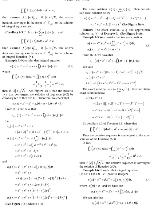
Example 6.4 Consider that integral equation

 

1



  

0 d

u x xx x 



xtt u t t (6.2) where

 

1 1





2

2

0 0

2

, d d d d

1 1 1 7

, 9 3 3 9

b b

a ak x t x t xt t x t

B

 

      

 

 

then if  3 7 (See Figure 1(a)) then the iterative

 

 that convergent the solution of Equation (6.2) by corollary 6.2 of theorem 6.1. Therefore, we check that





0( ) , 0 1, 0 1 .

u x xx x    

From (6.1), we have that

 

1



  

1 ₀ d

n n

u_ x xx x 



xtt u t t

Let

 



 

  





 

   









0

1 1 1

1

1 ₀ 0

1 _{1 1 2}

0 ,

2 2 3 , 0

d d

1 ,

u x x x x

u x x x x xt u t t

x x x t t t t

x x x x

x x x

                                                    





1 ,



, and

 

   









 













 





 



 

 

1

2 ₀ 1

1 1 1

2 2

d

2 2 3 1

1

1

1 n

n

u x x x x xt u t t

x x x

x

x x x x

x x x

u x x x x

                                                     



 

(See Figure 1(b), when n = 4).

The exact solution

 

lim _n



.

n

u x u x







Then we ob- tain exact solution below

 









2 2

1

1

1 (See ).

n n

u x x x x

x x x

 

 

    

  

       

    Figure 1(a)

 

Remark The exact solution u x  and approximate solution 4 of Example 6.4(See Figure 1(c)).

Example 6.5 We consider that integral equation

( ) u x

 





 

 





2 2 4 0 1 4 0 ,

0 1 .

d

xt t t

u x x x

u x x x u t

  



       



(6.3)

From (6.1), we have that

 

₄ 1



_{2 2}



 

1 ₀ d .

n n

u _ x xx 



xt t u t t

We take

 







  

 









1 4 0 4

2 2 3 3

0 1 , 3 1 7

1 .

n

n n

u x x x l

u x x x

x l l l l l

                          .

The exact solution

 

lim _n



,

n

u x u x







then we obtain exact solution below

 













 







 







4

2 2 3 1

2 4 1 4 1 1

1 1 .

n n

u x x x

x l l l l

x x l x l l

x x l x l

                                      

By corollary 6.2 of Theorem 6.1, where that

 

2 2

, d d , and .

b b

a ak x t x t B  B

1



   

 

Then the iterative sequence is convergent to the exact solution of the Equation (6.3).

In fact,

 

1 1





2

2 2 2

0 0

2

, d d d d

1 1 1 7

, 15 5 5 15

b b

a ak x t x t xt t x t

B

 

      

 

 

then if   15 7, the iterative sequence is convergent the solution of Equation (6.3).

Example 6.6 Consider that integral equation (0  1,0, kpositive integer),

 

₂ 1

   

0 d ,

k k

u x xx 



xt u t t (6.4) where u

 

0 0, and we have that

 

₂ 1

 

 

1

0 d

k k

n n

u x xx 



xt u _ t t

We can take that

 

2



0 0 1, 0

k k

[image:6.595.49.550.62.754.2]

0 500 1000 1500 2000 2500 3000 3500 4000 4500 5000 0

1 2 3 4 5 6 7 8 9

x

u(x

)

Solution of-eq, u(x)=xa+xb+0.4*sqrt(7)*x

(a)

0 500 1000 1500 2000 2500 3000 3500 4000 4500 5000 0

2 4 6 8 10 12 14

x

u4(x

)

Solution of-eq, u4(x)=xu4 a+xb+x[n]*(2/sqrt(7),1/sqrt(7)),a=0.2,b=0.5,n=4

u4

(x)

(b)

0 500 1000 1500 2000 2500 3000 3500 4000 4500 5000 0

0.2 0.4 0.6 0.8 1 1.2 1.4 1.6 1.8

x

ab

s

(u-u4)

absolute error abs(u(x)-u4(x)),a=0.2,b=0.5,n=4u4(x)),

u4

)

[image:7.595.170.422.79.688.2]

(c)

Figure 1. By Matlab in numerable test. (a) The figure expresses exact solution u(x) for Example 6.4; (b) The figure expresses approximate solution u4(x) for the solution u(x) of Example 6.4; (c) The figure expresses absolute erroru x( )u x4( ) for Ex-

(k-positive integer), and

 

   

















 

   































 



 

   

1 1

2 2 1 2 1

1 ₀ 0 ₀

1 1

2

1 2

2 ₀ 1

1 1 1

2 1 2 1 2

0

1 1

2 2

2

3 2

d d

2 2 2

d

2 2 2 d

2 2 2 1 3

k k k k k k

k k

k k

k k k k

k k

k k

u x x x xt u t t x x x t t t

x x x k k

u x x x xt u t t

x x x t t t k k t

x x k k x

u x x x xt u t

  





 





    

   

 

     

    

 

 

 

 

 

 

      

     

  

       

      

  























 





















 

 



1

0

1 1

2 1 2 1 2

0

1 1 2

2 2

d

2 2 2 1 3

2 2 2 1 3 1 3 .

k k k k

k k

t

2

3

d

x x x t t k k t

x x k k x

 



      

     



 

 

        

       





t

Inductively, we have

 

 

 













 

 

1 2

1 0

1 1 2 1

2 2 3

d

1

2 2 2 1 3 1 3

3

k k

n n

n

k k n

u x x x xt u t t

x x k k





 

      



  

  

 

      _     _

 



 x

Then by Theorem 6.1 and simple computation, we ob- tain that

 

1 1

 

2

2

0 0

1

, d d d d ,

9

b b

a ak x t x t xt x t B

 

 

2_{ }

then if  3, the iterative is convergent the solution of integral equation (6.4) (Similar as examples case in [6, 7]).

7. Some Effective Modification and

Numerical Test for [8]

In this section, we apply the effective modification me- thod of He’s VIM to solve some integral-differential equations. In [6-8] by the variation iteration method (VIM ) simulate the system of this form

 

. LuRuNug x

To illustrate its basic idea of the method, we consider the following general nonlinear system

 

,

LuRuNug x Lu

the highest derivative and is assumed easily invertible, is a linear differential operator of order less than,

represents the nonlinear terms, and

R

Nu g is the

source term. Applying the inverse operator 1

x

L to both sides of above equation, we obtain

 

 

1 1

.

x x

u f L Ru L Nu

The variational iteration method (VIM) proposed by

Ji-Huan He (see [6-8] recently has been intensively stud- ied by scientists and engineers. the references cited therein) is one of the methods which have received much concern. It is based on the Lagrange multiplier and it merits of simplicity and easy execution. Unlike the tradi- tional numerical methods. Along the direction and tech- nique in [4,8] we may get more examples below.

Example 7.1 (similar as example in [8]) Consider the following nonlinear Fredholm integral equation

   

cos 9 sin 9 sin 9 ,



0 0.

u x u x x xx x x u



 (7.1) Applying the inverse operator Lx1



to both side of Equation (7.1), yields:

 

_{sin 9 cos 9} 1 _{sin 9} 1

 

_.

9 81 x

x

u x x x x xL _u x _

from 1





0

sin x d cos sin cos .

x

L x x  



x x xx x So,





 

 

1

0

1

1 0

1 1

sin 9 d cos 9 sin 9 cos 9 .

9 36 9

sin 9 cos 9 sin 9

9 81

sin 9 .

x x

x x

L x x x x x x

x x

u x x x x x L f x

x x





   

    _ _





Inductively,

 

 

 

1 1

1

1

sin 9 cos sin 9 ,

9 81

sin 9 , 1.

n x

n

x

u x x x x x L u x

u x x x n

 



    _{ }

 

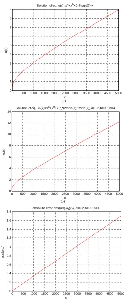
Then is exact solution of (7.1). The numerical results are shown in Figure 2.

 

sin 9

u x x x

Example 7.2 Consider the following Volterra-Fred- holm integral-differential equation

 



  

1



  

₃

0 0

ex x d

u x  



x t u t t



x t u t d ,t (7.2) Similar as example1 in this way, we easy get this solu-tion.

According to the method, we dividef into two parts defined 0

 

e ,

x

f x  and

 

   

 

 

1 3 , 0 1 .

f x  p x f x  f x  f x

By calculating this

 





3 3

2 3

e 1 e 1 1 2e

2 6 9

e 1 1.

x

x

p x x x

x

    

_  _ 

 

  

So, we have

 



  



  

1 0

1 3

0

e d

d

x x

x

x

x

u x L x t u t t

L x t u t t





 

  _  _

 

 

 _  _





In fact, in this way



  

















1 3 1

1 1 3

0

0 0

3 3

3 2

0

d e e d

e 1 1 e 1 1

2e 1 d 2e 1 ,

3 9 6 9

t t

x x

x

L x t f t t L x t 3 t

3

x x x

  _ _   _

  

  

   

 _   _   

 







x

 

and



  













1 1

0

0 0

2

d e e

e 1

e e 1 2

x x _{t t}

x x

x

x x

L x t f t t L x t t

x x

 _{ }  _



d

.

   





Writing

 

3 2 3





3

e 1 e 1 1 2e

e 1

2 6 9

x

x

p x     x   x x 1,

  

n

therefore, we have

 

 



  



  

1

1 3 ₀ 0

1 1

0 0

e d

d e , .

x x

x

x x

u x p x L x t f t t

L x t f t t





 

   _  _

 

 

 _  _

 







Inductively,

 

 



  



  

1

1 3 ₀

1 1

0

e d

d e ,

x x

n x

x

x n

u x p x L x t u t t

L x t u t t

 



 

   _  _

 

 _  _

 





And un

 

x e .x Hence the

 

e

x

u x  is the exact solution of (7.2).

Example 7.3 Consider the following integral-differ- ential equation

 ₅

 

1

 

0

4 3

ex d

x

u x   



xtu t t, (7.3) where u

 

0 1,u

 

0 2,u

 

0 1,u

 

0 1 In similar example1, we easy have it .

According to the method, we dividef into two parts defined by

0 500 1000 1500 2000 2500 3000 3500 4000 4500 5000

-5 -4 -3 -2 -1 0 1 2 3 4 5

x

u(x

)

[image:9.595.57.534.68.711.2]

Solution of-eq, u(x)=x*sin(9*x)

 

 

 

 













0 0 0

6 6

1

e , e ,

4 3 6! 2 540 .

x x

f x x u x f x x

f x x

    

     x

Taking f x

 

 x ex



1 540



x6, then we have

 





_{6 1} 1

 

1 e 1 540 ₀ 0 d

e ,

x

x x

u x x x L xtf t t

x

  

    _{ }

 



where 1

 

 

0 0 0 0 0

· x x x x x · d d d d d .

x

L 

    

t t t t t

And the processes,

 





_{6 1} 1

 

1 e 1 540 ₀ d , 1

x

n x

u_ x  x  x L _ xtu t t_ n





n  .

Thus, 1

 

e ,

x n

u _ x  x then _{u x}

 

_{ x} ex

is the exact solution of (7.3) by only one iteration leads to a solution. The numerical results are shown in Figure 3.

Example 7.4 (See example 2 in [8]) Consider the fol-lowing partial differential equation

e .

k k x

t x

u uu ax t b (7.4)

Let that integer The modified meth- ods:



1, , 0 ,

k a b



Applying the inverse operator to both sides of (7.4) yields

 

2 1 1 1 2

 

, ,

2 1 2

k k k k

x _x

b

u x t ax t x t L u x t

k

  _{ }

   _{ }



where 1

 

 

0

· x ·

x

L 



d .t

Here, we divide f into two parts defined by

 

 

 

2 1

0 1 0 1

1

, ,

2 1

k k k

Using the relation 9 9 , we obtain

k k u  f ax t

 

 

 

0

2 1 1 2

1 0

, ,

1

, ,

2 1 2

,

k k

k k k k

x _x

k k

u x t ax t

b

u x t ax t x t L f x t

k

ax t

 



 

   _{ }

 

and so on

 

2 1 1 2

 

1

1

, ,

2 1 2

, 1.

k k k k

n x n _x

k k b

u x t ax t x t L u x t

k

ax t n

 

   _   

 

Hence, u x t

 

, ax tk k

1, 1

k a b

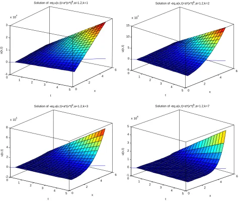
is the exact solution of (7.4) and by only one iteration leads to that exact solution. Taking    that is example 2 in [8].

The numerical results are shown in Figure 4.

Remark 7.5 Some solving integral-differential equa-tions by VIM may see [9], and that some random Altman type inequality for fixed point results see [10].

The fixed point results of Multi-value mapping are also discussed in [11].

Remark 7.6 By [12], the authors consider the mixed problem for non-linear Burgers equation:

    



 

 

 

   





2

2, , 0,1 0, ,

, 0 , 0,1 ,

0, 1, 0, 0, .

u u u

u x t

t x x

u x x x

u t u t t





  

   

   

 _{ }



 _{   }

 



(7.5)

.

f ax t f xt f x f x f x

k



   



The authors point out the problem describes physic phenomenon of motive quality and conservation of law in dynamic problem, it is important model in flow me- chanics. Where u express the velocity of flow body,

0 500 1000 1500 2000 2500 3000 3500 4000 4500 5000 0

100 200 300 400 500 600 700 800

x

u(x

)

[image:10.595.148.434.497.715.2]

Solution of-eq, u(x)=x*exp(x)

0 1

2 3

4

5 0 2

4 6 -1

0 1 2 3

x 104

x Solution of -eq,u(x,t)=a*(x*t)k,a=1.2,k=1

t

u

(x

,t)

0 1

2 3

4

5 0 2

4 6 -5

0 5 10 15

x 104

x Solution of -eq,u(x,t)=a*(x*t)k,a=1.2,k=2

t

u(

x

,t

)

0 1

2 3

4

5 0 2

4 6 -2

0 2 4 6 8

x 105

x Solution of -eq,u(x,t)=a*(x*t)k,a=1.2,k=3

t

u(

x

,t

)

0 1

2 3

4

5 0 2

4 6 -1

0 1 2 3 4 5

x 108

x Solution of -eq,u(x,t)=a*(x*t)k,a=1.2,k=7

t

u(

x

,t

[image:11.595.62.539.84.483.2]

)

Figure 4. Figures of exact solution u(x) for example 7.4. (where parameters taking as a1 2. ,k1 2 3 5, , , ). and  express the constant of motive flow body,

 

x

 -initial function.

Burger’s equation has attracted much attention. The approximation solution for this Burger’s equation is also interesting tasks.

8. Concluding Remarks

In this Letter, we give out new fixed point theorems in cone metric space and apply the variation iteration me- thod to integral-differential equation, and extend some results in [3,6-8]. The obtained solution shows the me- thod is also a very convenient and effective for some various non-linear integral and differential equations, only one iteration leads to exact solutions.

Recently, the impulsive differential delay equation and stochastic schrodinger equation is also a very interesting topic, and may look [11] etc.

9. Acknowledgements

This work is supported by the Natural Science Founda- tion (No.07ZC053) of Sichuan Education Bureau and the key program of Science and Technology Foundation (No.07zx2110) of Southwest University of Science and Technology.

The authors would like to thank the reviewers for the useful comments and some more better results.

REFERENCES

[1] D. J. Guo and V. Lakshmikantham, “Nonlinear Problems in Abstract Cones,” Academic Press, Inc., Boston, New York, 1988.

[3] X. Zhang, “Common Fixed Point Theorem of Lipschitz Type Mappings on Cone Metric Space,” Acta Mathe-matica Sinica, Chinese Series, Vol. 53, No. 6, 2010, pp. 1139-1148.

[4] H. Avdi, H. K. Nashine, B. Samet and H. Yazidi, “Coin- cidence and Common Fixed Point Results in Partial Or- dered Cone Metric Spaces and Applications to Integral Equations,” Nonlinear Analysis, Vol. 74, No. 17, 2011, pp. 6814-6825. doi:10.1016/j.na.2011.07.006

[5] S. H. Cho and M. S. Kim, “Fixed Point Theorems for General Contractive Multi-Valued Mappings,” Applied Mathematics Information, Vol. 27, No. 1-2, 2009, pp. 343-350.

[6] N. Chen and J. Q. Chen, “New Fixed Point Theorems for 1-Set-Contractive Operators in Banach Spaces,” Journal of Fixed Point Theory and Applications, Vol. 6, No. 3, 2011, pp. 147-162.

[7] N. Chen and J. Q. Chen, “Operator Equation and Appli- cation of Variational Iterative Method,” Applied Mathe- matics, Vol. 3, No. 8, 2012, pp. 857-863.

doi:10.4236/am.2012.38127

[8] A. Ghorbani and J. Sabaeri-Nadjafi, “An Effective Modi- fication of He’s Variational Iteration Method,” Nonlinear Analysis: Real World Applications,Vol. 10, No. 5, 2009, pp. 2828-2833. doi:10.1016/j.nonrwa.2008.08.008

[9] S. Q. Wang and J. H. He, “Variational Iterative Method for Solving Integral-Differential Equations,” Physics Let- ters A,Vol. 367, No. 3, 2007, pp. 188-191.

doi:10.1016/j.physleta.2007.02.049

[10] N. Chen, B. D. Tian and J. Q. Chen, “Some Random Fixed Point Theorems and Random Altman Type Ine- quality,” International Journal of Information and Sys- tems Sciences,Vol. 7, No. 1, 2011, pp. 83-91.

[11] S. Jain and V. H. Badshah, “Fixed Point Theorem of Multi-Valued Mappings in Cone Metric Spaces,” Inter- national Journal of Mathematical Archive, Vol. 2, No. 12, 2011, pp. 2753-2756.

[12] J. Biazar and H. Aminikahah, “Exact and Numerical So- lutions for Non-Linear Burgers’s Equation by VIM,”