Super Resolution with Multiselective Contourlets

Super-Resolution with Multiselective Contourlets

Mohamed El Aallaoui1, Abdelwahad Gourch2

1_{Laboratory of Mathematical Engineering (LINMA), Department of Mathematics and Computer Science,}

Faculty of Sciences, Eljadida, Morocco

2_{Faculté des Sciences Juridiques, Économiques et Sociales de Ain Sebaâ, Casablanca, Morocco}

Email: m_elaallaoui@yahoo.fr, agourch2002@yahoo.fr

Received July 18,2012; revised September 19, 2012; accepted October 10,2012

ABSTRACT

We introduce a new approach to image super-resolution. The idea is to use a simple wavelet-based linear interpolation scheme as our initial estimate of high-resolution image; and to intensify geometric structure in initial estimation with an iterative projection process based on hard-thresholding scheme in a new angular multiselectivity domain. This new do-main is defined by combining of laplacian pyramid and angular multiselectivity decomposition, the result is multiselec-tive contourlets which can capture and restore adapmultiselec-tively and slightly better geometric structure of image. The experi-mental results demonstrate the effectiveness of the proposed approach.

Keywords: Super-Resolution; Laplacian Pyramid; Angular Multiselectivity; Multiselective Contourlets; Anti-Aliasing

Filer; Sparsity Constraint; Iterative Projection

1. Introduction

In most digital imaging applications, high-resolution im- ages or videos are usually desired for later image proc- essing and analysis. The desire for high resolution stems from two principal application areas: improvement of pictorial information for human interpretation; and help- ing representation for automatic machine perception [1,2]. Image resolution describes the details contained in an image, the higher the resolution, the more image details [1,3]. Super-resolution is techniques that construct high- resolution images from several observed low-resolution images, thereby increasing the high-frequency compo- nents and removing the degradations caused by the im- aging process of the low-resolution camera. The basic idea behind super-resolution is to combine the non-re- dundant information contained in multiple low-resolution frames to generate a high-resolution image. The super- resolution (SR) reconstruction of a digital image can be classified in many different ways: SR in spatial domain [4,5], SR in the Frequency Domain [6,7], Statistical Ap- proaches [8,9], and Interpolation-Restoration [1,10]. In this last context, can be distinguished two categories, linear and nonlinear interpolation methods.

Linear interpolation methods, such as bilinear, bicubic and cubic spline [11,12], edge-sensitive filter [13], blur- ring and ringing effects because they do not utilize any information relevant to geometric structure of image [14,15]. Nonlinear interpolation methods incorporate more adaptive image models and priori knowledge which

often improve linear interpolators. Many approaches have been designed for addressing this task in recent years. We may cite for instance, Soft-decision Adaptive Interpolation (SAI) [16], Sparse Mixing Estimators (SME) [17], Iterative Projection [18], ···

scheme in a new angular multiselectivity domain. This new domain is defined by combining of laplacian pyra- mid and an angular multiselectivity decomposition. The result is new multiselective contourlets, which can rep- resent the different structures of the image geometry.

The paper is organized as follows. In Sections 2 and 3, we discuss the new multiselective contourlets, and we will show how these multiselective contourlets can pro- vide a new degree of freedom to describe adaptively the different structures of the image geometry. Our multise- lective contourlets algorithm for image super-resolution is described in the Section 4. We report the results of our experiments in Section 5 and conclude the paper in Sec- tion 6.

2. Laplacian Pyramid

The Laplacian Pyramid was first proposed in [22] as a new technique for compression image. To achieve high compression, it removes image correlation by com- bining predictive and transform coding techniques.

 

LP

In the Laplacian Pyramid decomposition at each level the original image happens in a high-pass and a low-pass filters, the resulting is a downsampled low-pass version of the original image, and of difference between the original image and the prediction.

Under certain regularity conditions, the low-pass filter

g in the iterated LP uniquely defines a unique scaling

function that satisfies the following two- scale eq

 

2



2

t L

  



uation [23,24]

 

2

 

2



2



n

t g t

 







n . (1)

Let

 

2

,

2

2 , ,

2

j j

j n j

t n

t j

 _     _

 

  n . (2) Then the family is an orthonormal basis fo

 

j n, _n 2

r an approximation subspace Vj at the scale 2

j_. Furthermore,

 

Vj _j provides a sequence of multire-

solution nested subspaces _V2  V1 V0 V1V2_, where Vj is associated with

2 2

a uniform grid of intervals j_ j _{that characterizes image approximation at scale} 2j_{. Th}

nec

e difference images in the LP contain the details

essary to increase the resolutio etween two conse- cutive approximation subspaces. Therefore, the diffe- rence images live in a subspace

n b

j

W that is the

orthogonal complement of Vj in Vj1, or

1 .

j j j (3)

The can be considered as an oversampled filter

ba here

V V W

LP

nk w each polyphase component of the difference signal comes from a separate filter bank channel like the coarse signal [25]. Let F zi

 

,0 i 3 be the synthesis filters for these polypha . Note that these synthesis filters are high-pass filters. As for wavelets, we associate with each of these filters a continuous function

se components

 

i

t

 where

 



2

2 i 2

n

t f

 





.

n

i

t







): let

(4)

osition 2.1 ([25] Prop

 

2

,

2

2 , ,

2

j i j i

j n j

n

t j

 _    _

 

  n . (5)

, for scale

t

 

Then 2j_,

 

2

, _{0 3,}

i j n _{i n}



   is a tight frame

for Wj.

Since W_j is generated by four kernel functions

(similar to multi-wavelets), in general it is not a shift- invariant subspace. Nevertheless, we can simulate a shift- invariant subspace by denoting

 

i

t

 _,2 _,

 

,0 3.

i

j n k  j n t  i (6)

are the coset representatives for downsam

T

T (7)

this notation, the family associated where

With to a

i

k

i

p- ling by 2 n each dimension

 

T

0,0 ,

k 

 

 

 

0 1

T

2 3

1,0 ,

0,1 , 1,1 .

k

k k



 

 

j n, _n 2

1 1

n uniform grid of intervals 2j _2j _{on }2 _pro-

vides a tight frame for Wj [25]. Then the amily f

 

j n, _n 2 suffices the following equality:

2

2 ₂

, , .

n j j

n

f f f W





  



(8)

elective Contourlets

elective contourlets

eriodic function

3. Multis

In this section we propose the multis

defined by combining of laplacian pyramid and an angu- lar multiselectivity decomposition, and we will show how these new contourlets can provide a new degree of freedom to describe adaptively the different structures of the image geometry.

We consider 2π-p  defined by

 

















, 0 , 2 ;

1, 2 ,π ;

π

, π,π 2 ; 0, π 2 , 2π .



 

  



 

 

 

  



 

    _

 

 _{ }



 



  _{ }

 

 _{ }

 

  



  

 

0,π

 and the function 

where is defined in



1,1



and satisfies the following property:

 

 

2 2 _1.

t t

   

For and

(10)

*

L π

2L

  , we create 2l _{different -}

periodic functions

2π

,

l m

 indexed by for any

de

0 2l

m

 



0,



l ,L fined by:

 

0,0 1,

   (11)

 

 





1,2 ,

2 1 π

,

l

m

 

 

   ) 2

l m l m 

_    



(12 

 

 





1,2 1

l m

_{ }  _,

π . 2

l m l 

  

 

 

_   _

 

By the laplacian pyramidc wavelets

2m1 π (13)

,

j n

 bspace

defined in the previous section and for each su Wj

r transf , we construct a new contourlets whose Fouri orms are:

e

 

 

 

, , , , ,

ˆj n l m ˆj n l m ,

 k  k  

where

(14) arg

 k.

osition 3.

Prop 1 for any l



1, , L



 





,0

l

 

 

1

1

1 1

1

, 0 , 2 ;

π

1, 2 , ;

2

π π

2 _{, , 2 ;}

2 2

π

0, 2 , 2π .

2

l l

l l l

  



 

π _{ }

  



 

 

 





 

 _{ }



 _{ }



 _{ }

 



  _{ }

 _{   }

 

 _{   }

 

  



 _ _ 

 _ _



(15)

and

   

  

   



0, , 2l 1



m

  _ 

 

 

 

 

, , , , ,

, ,0

ˆ ˆ

2π

ˆ .

2 j n l m j n l m

j n l m l

   

  



 

 _  _

 

k k

k (16)

Proof

According to the expression (9) of the function _,

π 2

π

0, 0 , ;

2 π

π π

2 _{, , 2 ;}

2 2l l



π π

1, 2 , π ;

2 2

π

π+ _{π π}

2 _{, π, π 2 ;}

2 2

π

0, π 2 , 2π .

2 l

l

l

l l

l

l l

l

 



 

 

 

  



one have for any l



1, ,_ L



:

  



 

 _ 

 

 

 _ 

 _ _



 _{ }

 

  _{ }

 

 



  

 _   _

 



  _{ } 

   _{ }

 _{      }

 _{ }  

  



 

 _{  }

 

 _{ }



(17) 

 _{ }

 

 _ _  _



π π

2

π

1, 0 , ;

2 π

π π

2 _{, , 2 ;}

2 2

π π

0, 2 , π ;

2 2

π

π _{π π}

2 _{, π, π 2 ;}

2 2

π

1, π 2 , 2π .

2 l

l

l

l l

l l

l

l l

l



 



 

  



  

 

 



 

 _{ } 

 

 

 _ 

 _ _



 _{ }

 

   _{ }

   _  _

 

 _ _

 _{ }



  

 _  _

 



  _{  } 

   _{ }

 _{      }

 _{ }  

  



 

 _{  }

 

 _{ }



 

(18)

We shall now prove that for any l



1, ,_ L



 





1

,0 ₁

1 1

1

, 0 , 2 ; π

1, 2 , ;

2 π

π π

2 _{, ,}

2 2 π

0, 2 , 2π .

2 l

l

l

l l

l

 

  



 

  _{ }

2 ;

  



 





 



    _

 

 _{ }



 _{ }



 _{ }

 



  

  _   _

 

 _{   }

 

 _{   }

 

  



 _ _ 

 _ _



(19)

Let’s prove this by induction: Since

 

  





1,0 0,0  π π 



expressed as (19). Now assume that for a fixed , the function

l

,0

l

 n h

expressed as (19). The inclusio this inductio ypothesis and Equation (18) in the ex- pression (12) gives:

n of

 





1,0

, 0 , 2 ; π

1, 2 , ;

2 π

π π

2 _{, , 2 ;}

2 l

l

l

l l

 

  



 

  _{ }

  



    _

 

 _{ }



 _{ }



 _{ }

 



  

  _   _

 

 _{   }

 _

 

(20)

e expressions (17) and (19) in Equation (13) shows that: for any

2 

 _{  }

 

 _

π

0, 2 , 2π .

2l

 

 _ _ 

 _ _



This last result completes the proof of the induction. The insertion of th



1, ,



l _ L

 

1

1

1 1

,1 1 2

2 _{π π}

2l _{, , 2 ;}

2 2

2l 2l

2

π

0, 0 , ;

2 π

π π

2 _{, , 2}

2 2

π π

1, 2 , ;

2 2

π

π

0, 2 , 2π .

2 l

l

l l

l l l

l



 

;

  



   

 

     

   _{ }

 _{   }

    

 _{ }  

  



 





 

 



 _ 

 _ _



  _{ } 

   _{ }

   _  _

 

 _ _

  



  

 _  _

 



  

 

 _{ }

 

 _{ }



(21)

Therefore, for any l



1, ,_ L



 

,1 ,0 1

π . 2

l l l

   _ _ _

  (22) We shall now prove that, for any L



(23) Let’s prove this by induction:

Now assume that for a fixed

 (24)

with



1, ,

l _

 





, ,0 , 0,1, , 2 1.

l l m l l m m

      _ 

l:

 





, ,0 , 0,1, , 2 1

l l m l l m m

      _

,

2π_. 2

l m l

The inclusion of th

 

 









m

 

e induction hypothesis and Equ- ation (22) in the expressions (12) and (13) gives:









1,0 1,2

l l m

_  _

 

1,2 ,

,0 , ,

1,2

2 1 π

2 π π

2 π

2 ,

l m l m l

l l m l m l l m l

m 



     



 







 

 _   _

 



 

 

 _{  } 

 

 

,0 1,2

l l m 

  _ 

 

π

π     

  _  _

 

 





















1,2 1 ,

,0 1,2 1,2

1,1 1,2 1,0 1,2 1

2 1 π 2

π

2 .

l m l m l

l l m l m l

l l m l l m

m 



     

     

     

 

 

    



 

 _  _

 

 

  _   _

 

    

The proposition shows that for each level of con- struction l, the functions

,0 , ,

2 π

l l m  l m l

     

  _   _

 

 

,

l m

 are continuous with co - pact support of size

m 2π

2

2l  . So the aperture of the

cone in frequency space supporting of ˆj n l m, , , is equal

to 2π 2

2l  . Therefore, the contourlets j n l m, , , are

directional [26,27], and the angular selectivity of these new contourlets is proportional to . Keeping that in mind, we will call the new cont

2l

ourlets j n l m, , , the mu

tiselective contourlets, and the param angular selectivity level.

The central result is that for each selectivity level the multiselective contourlets generate a tight frame each subspace

l-eter l the

l,

for

j

W .

Theorem 3.1 for any l



0, ,_ L



the family



2



, , , : , 0,1, 1

l j n l m n m

   _, 2  is a tight frame for

j

W .

Proof

To prove that the family



2_{, 0,1, , 2}l ₁



m

j n l m, , , :n    is a tight frame for

j

W , it suffices to evaluate the equality:

2

2 1 2

, , , 0

, .

l

2

j n l m j

m n

f f f W





 

  

 

(25)

Define the quantities

 

2

2 1 2

, , , , 0

,

l

j n j l m m

n

E f  f



 



 

(26)

and



j n l m, , ,



 

ˆj l m, ,

 

ˆ

 k  k j l m, ,



2jn



. 

k (27)

 

E f





  

2 1 2 ˆ 4π l f  



 



2  k k



fˆ



k2jn



d .k(28)

2 _m0 j n l m, , ,

n  

We have

 

 

d d

f  f







x x x

 

 

 





 





   



 

 

     

2 2 2 2 2 2 2 , , , , , , , , , , , , , , i2 , , i2 , , , , 2 d 2 d ˆ ˆ e d d ˆ ˆ ˆ ˆ e d j j

j n j l m

j n l m j n l m j

j l m

j j l m n

j l m n

j l m j l m

f f n f n f f f                         





 

            k k k

x x x

x x x

x x x

k k k

k

k k k k k k

Using the Poisson formula

(29) We obtain

. We shall now prove that

(30) According to the property (10), we verify that

(31)

  

2

i2

, , ˆ

ˆ e j_n

j l m f



 _





_ k 

k k 2 



_ d .  





2 2 i2 2

e jn 4π 2j .

n n n        



k k



k k

 





   





2 2 2 1 2 , , , 0 ˆ ˆ

4π 2 d

l

j j n l m

m n

E f

f f n



  



 



_   

k k k k





 

 





2 1 , , , 0

ˆ ˆ 2 .

l

j j n l m j j m n        





k k k

 





2 2 _{π 1.}

 

    

Hence, for any l



0, , L







 





 









 









 

 

 









 

1 2 1

, 1, ,0, 1,

ˆ ˆ 2

l

j l m j l m

 



 





 

k



k



1

0 2l 1

 

1

2 1 , , ,

, ,2 , ,2

0

, ,2 1 , ,2 1

2 1

2 , 0

2

, 1, , 1, ,

0

ˆ 2

ˆ 2

2

ˆ ˆ 2 π

l

l

j n l m m

j j l m j l m m

j j l m j l m

j

m l m

j

j l m j l m m l m n n n n                            _     _     _{ }





   k k k k k k k k

, 1, , 1,

ˆ_{j l m} ˆ_{j l m}

 _  _







_ 

k

 





 





1





 

2 2

,

2 1

, 1, , 1, , , 1,

0 0

π

ˆ ˆ 2 ,

l

m l j

j l m j l m j n l m

m m n                   _{ } 



  





k k k

with

1

, 2l 1

m l  _{ }  j n





, 1

2 1 π

. 2

m l l

m    _

Therefore,

The equalities (8), (26), (28) and (30) imply that





 





 

 





2 1

, , , , ,0,0

0

ˆ ˆ 2

l

j j n l m j n j j m n           



k k k  k

 





 





   

   

 

 

 

 

2 2 2 2 2 2 2 2 2 2

2 1 2

, , , 0 2 i2 i2 , , 2 ₂ , , ˆ ˆ ˆ ˆ

4π 2 2

ˆ ˆ

ˆ ˆ

e d e

d d

.

l

j j

j n l m m

n

j j

j j j j

n

n n

j j

n

j n j n

n j n

d

d

f

n f f n

f f f f f f                            

 

 

 



 





            k k

k k k k k

k k k k k k

x x x x x x

fore, for each selectivity level , any function

n

There l

j

f W is represented as:

 

2

 

2 1 , , , , , , 0 . l

n j l m j n l m m

n

f  f 



 



 

x x (32)

Since



J



0 0

j J j

V V 



_jjW , any f Vj₀ is repre- sented as:

 

 

 

2 2 2 ₀ , , 1 , , , , , , 0 ,

J n J n n

J l

j n l m j n l m j j m

n

f  

        



  

x x x (33) with , , ,

J n J n f

   (34)

, , , , , , ,

j n l m j n l m f

   (35) and t

orthogonal s

im t for each selectivity le the the he decompositions of 2

 

2

L  into mutual

ubspaces:

 

2 2 _,

J j

j J

L V W



 

 _{  }





 (36)

ply tha vel l, family



2



, : , , 0,1, , 2

l m n j J m

, , , , 1

J n j n l

     _  is a tight

frame for 2

 

2

L  , on which any function f L2

 

2

is represented as:

 

 

 

2 2 2 , , 1 , , , , , , 0

J n J n n

l

j n l m j n l m j J m

n

f  

sition of 2

 

2

f L  is

ficients The multiselective decompo

defined as the set of the coef j n l m, , , up to a

scale J

req

and a selectivity level low-f uency information

L plus the remaining

,

J n

 :



j n l m, , ,



_{j J}



 

 _,n 2_{,0m<2 ,0}l _{ l L},



J n, _n 2 . (38)

Since the multiselective contourlets de image with the different selectivity level this multiselective decomposition represen

for each level , theorem

the multiselec



compose the



0,1, ,



 _ ,

l L

ts and captures , 2.1 s

different structures of the image geometry. In particular



0,1, ,



l _ L

tive contourlets

hows that

, , ,

j n l m

 whi

ut there is more. Indeed, as shown in the following proposition, we can mix different frames inside the same reconstruction formula.

Proposition 3.2 for any function:

generate a tight iginal image frame, on ch we can reconstruct the or

according to (37). B













2 0, : , , , j J j j       

x x (39)

any we obtain the following reconstruction for f vj₀

 

 

2 J n, J n,

n

f  

 



x x

 

2 2 0 1 , , , , , , 0 , J

j n m j n m j jn m

 

   



  

 _{ } x

(40)

with

, , ,

J n J n f

   (41)

, , , , , , .

j n m j n m f



We shall now prove that, for any  

  (42)

Proof

Define the quantity

  

f 2 1j n, , ,mj,

 

. 

 

 





x x (43)

2_{m 0}

n 

, ,

nm



 :

  



2 j n, j n,

n

f  



 x 



x



. (44)

We have

 

 

 

 

 

 









   



2



 

ˆ d j_n   k k k

   

2 2 2 2 2 , , , , , , , , , , , , , , , , , , , , , , i i2 , , , , i2 i2 , , , , d

2 d 2

ˆ ˆ

e d e

ˆ

ˆ ˆ

e d e

j

j j

j n m j n m j n m j n m

n j m n j m

j j

j m j m

n

j m j m

n n

j m j m

f f n n f f                              











                   x k k k x x

x x x x

x x x x

k k k

k k k

 

   

i

, , ˆ

ˆ e d d .

j_n

j m f



 _{ }  _



k k xk

k k k k k

Using the Poisson formula

(45) and the equality (30), we obtain:

 

_eixk

k dk

2f







 

i2

 

2 2e ˆj, ,m



 

_

 

 





i2 2

e jn 4π 2j .

n



 _{  }



k k



k k

2 2

n n

  

 





 





 





 





 





 





2 2 2 2 2 2 2 2 1 2 , , , , 0 i 2 2 1 2 , , , , 0 i 2 i 2 2 i2 ˆ ˆ ˆ 4π 2 e d ˆ ˆ ˆ 4π 2 e d ˆ ˆ ˆ

4π 2 e

ˆ e j j j j j

j m j m

m n

n

j

j m j m

m n n n j j j n n j f n f n f n f                                                 2 d n     _  _ 

  







 

 

             x k x k x k k x

k k k

k

k k k

k

k k k

   

 

   





 

 









 

 

 

  k

 

 

2 2 2 2 2 2 2 d j n f n 

 

 x x x

2 2 2 2 i2 i i 2 , , , , , ,

ˆ _{d e ˆ e d}

ˆ ˆ

e d e d

2 d = . j j n j n j j n j j j

j n j n

n

j n n j j n j n

n n f f n f f                                   



 



 





      k xk x k

k k k k k

k k k k

x

x x x x

x x

Since, we have for any

i2j_{nk } ˆ

k

0

j

fv

x (46)

we obtain the following reconstruction for any

 

 

 

2 , , ₀ 2 , ,

.

J

J n J n j n j n j j

n n

f    

   





 

x x 0 j

fv

x

The reconstruction carried out in this proposition pro- vides a new degree of freedom to describe images adaptively. Indeed, at each point and each scale we may search the adaptive ity reconstruction, at is, the selectivity level at improves the detection of the content of

 

 

2

 

2 2 0 1 , , , , , , , , 0 . J

J n J n j n m j n m j j m

n n

f    

     





  

 _{ }  x x 2  x selectiv



x,j



th

j,

th 

f .

4. Image Super-Resolution via Multiselective

Contourlets

The main idea is similar to the technique of interpolatio proposed in [18]. Our algorithm of image super-resolu-

tio e two constraints.

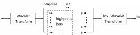
4.1. Anti-Aliasing Filer Constraint

an estimation xˆ0 of high-resolution image x from low-

resolution image xL (refer to Figure 1). In this case we

impose anti-al filer constraint, that is the given low-resolution i e is the downsampled output of the lo

iasi m

ng ag

w-pass anti-aliasing filter in a wavelet transform. As a simple way to get an estimate xˆ0 of the high resolution

image, we can take the inverse v et transform by k eping

wa el

e xL as the low-pass band and zeropadding all

high-pass subbands. Consequen r any given image y,

we can calculate the best approx 2

L norm) to

y, subject to anti-aliasing filer con

tly, fo imation (in

straint, through orthogonal projection. Let F and F1 represent the

forward and inverse wavelet transforms, respectively; ote P as the di

den onal 1s and 0s

sforms, culated by (47) e

n

de

multiselective contourlet coefficients.

ag projection matrix of

that keeps the low-pass wavelet coefficients and zeros out the high frequency subband coefficients, and let

P  I P. If we use orthonormal wavelet tran

then the projection of any image y can be cal





1

ˆ_   _ ˆ

0 ,

y F P Fy PFx

where

x

ˆ

₀ is th estimation of the high-resolution image obtained as in Figure 1.

4.2. Sparsity Constraint

The second constraint is based on a model for natural images. Since the multiselective contourlets described in Section 3, generate a multiselective geometric represen- tation well-suited to preserve contours and edges and geometric structure of image, we assume that the un- known high-resolution image should be sparse in the multiselective contourlets domain. For the sake of sim- plicity, we choose to use a direct hard-thresholding scheme i our proposed algorithm. Intuitively, we view our estimate to the high-resolution image as a noisy ver- sion of the true image. Enforcing our sparsity constraint works to noise the estimation of the interpolated signal while retaining the important coefficients near edges. we enforce this constraint through a hard-thresholding of the We suppose that the estimation ˆx of the high-

resolution is a multiresolution approximation of the real image f at the resolution 20. Hence xˆV0,



and the

om of

multiselective contourlets dec position xˆ is ficients

defined as the set of the coef

, , , , , , ˆ

j n l m j n l m x

[image:7.595.61.285.658.714.2]

   up to a scale J 0 and a sele-

Figure 1. The anti-aliasing filer constraint.

ctivity level L0, plus the remaining low-frequency information J n,  J n, xˆ :



, , ,



_{0 ,} 2_{,0 2 ,0}

 

, 2

ˆ _{j n l m l} , _{J n} .

n j J n m l L

x _ _{      }  _ _

 (48)

Denote T as the diagonal matrix that, given some

threshold value T, zeros out insignifica t coefficients in

the coefficient vector whose absolute values are smaller than T; and  as the adaptive selectivity reconstruction

given by proposition (3.2),

n

 

, ,

 

ˆ J n J n

x   

 

2

2 _{1 0} , , , , , ,

.

n

j n m j n m j m

n

 

   



2 ₁

J 



 

  t

 (49)

 t t

we choice the adaptive selectivity level by mini- mizing the distortion introduced by thre in fixed selectivity procedure:

 

j,

 t

sholding

 

_{ }

 

 

2 2

L

n n

with

, ,0,0 , , ,0

0,

, arg min j n j n l

l  









t t t ,

j

 (50)

 

2 1





 

, , ,0 , , , , , ,

0

.

l

j n l T j n l m j n l m m

   









t t (51)

Denote x_ the denoised high-resolution image. The

sparseness constraint by hard-thresholding can be written as

ˆ.

T

x x (52)

4.3. Multiselective Contourlets Algorithm for Image Super-Resolution

We show in Figure 2 the block diagram of the proposed

r

high-thm by taking

multiselective contourlets algorithm fo resolution image reconstruction, which can be summarized as fol- lows:

1) We start our algori xˆ0, obtained by

the simple wavelet interpolation shown in Figure

the initial estimate of the high-resolution image.

2) We then attempt to improve the quality of inter- on, particularly in regions containing edges and contours, by iteratively enforcing the observation con- straint as well as the sparseness constraint. Let

1, as

polati

ˆ_k

x re-

present the estimate at the kth step. By comb and (52), the

ining (47) new estimate xˆk₁ can then be obtained by





1

1 0

ˆ ˆ ˆ .

k

k T k

x_ F P F  x PFx (53)

3) Following the same principle o

based image recovery algorithm proposed in [28], we all amo

f the sparseness- gradually decrease the threshold value T_k by a sm

unt  in each iteration, i.e., Tk1 Tk 

rcum ng t

  venti

[image:8.595.306.540.83.252.2]

Figure 2. The block diagram of the proposed algorithm for image super-resolution.

convexity of the sparseness constraint.

We compare the high-resolution images obtained by the proposed method with those obtained by wavelet linear [28], interpolation bicubic [29], contourlet transform [18], soft-decision adaptive interpolation (SAI) [16], and sparse mixing estimators (SME) [17]. In the experiments, we use five scales J = 5, and five selectivity level

4) Return to step 2 and keep iterating, until the gene- rated images converge or a predetermined maximum iteration number has been reached.

5. Numerical Experiments

5

L

d we for multiselective contourlets decomposition, an choose T010 and is decreased by  0.2

erations 512

in each . We use 2 , in-iterati a maximum of 10 it

several rd test images of size

cluding Lenna, Boat, Gauss disc, Peppers, Straws, and

gular regions. Peppers is mainly composed of regular Mandril is rich in fin

ms, we first down- sampled each image by a factor of 2 and then inter-

on, with

standa 51

Mandril (Figure 3). Gauss disc image includes regular

regions, Lenna and Boat include both fine details and re

regions separated from sharp contours.

e details. Straws image contains directional patterns that are superposed in various directions. To show the true power of the interpolation algorith

polated the result back to its original size.

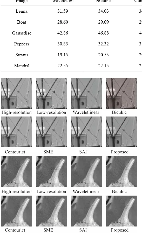
The performance measure used was the Peak Signal to

Noise Ratio (PSNR), A good high-resolution method

must maximize the PSNR. Table 1 gives the PSNRs

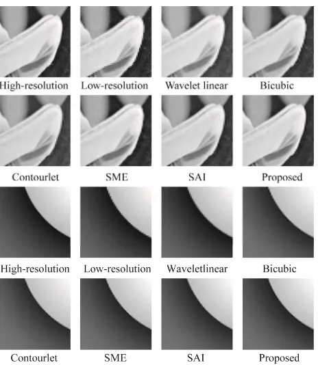
generated by all methods for the images in Figure 3. Figures 4 and 5 compare the high-resolution image

obtained by different methods. Bicubic interpolations produce some blur and jaggy artifacts in the zoomed images, but the image quality is lower than with SME and SAI methods, as shown by the PSNRs. The Con- tourlet method yields almost the same PSNR as a bicubic interpolation but often provides better image quality. It is able to restore the geometrical structures (see Lenna’s hat and gauss disc zoom) when the underlying contourlet

Figure 3. Images used in the numerical experiments.

Figure 4. The zoom-in comparison of the Lenna and Gauss disc images. From left to right: high-resolution image, low- resolution image (shown at the same scale by enlarging the pixel size), wavelet linear, bicubic interpolation, contourlet, SME, SAI, and proposed method.

[image:8.595.59.282.83.218.2] [image:8.595.309.541.276.543.2]

[image:9.595.55.295.132.527.2]

Table 1. The performance of the proposed method relative to oth of Figure 3. From left to right: wavelet linear [28], interpolat estimators (SME) [17], and soft-decision adaptive interpolation (S

Image Wavelet lin Bicubic Contour Proposed

er methods. PSNRS (in decibels) are computed over images ion bicubic [29], contourlet transform [18], sparse mixing

AI) [16].

let SME SAI

Lenna 31.59 34.03 34.17 34.61 34.74 35.10

Boat 28.60 29.09 29.1

Gaussdisc 42.86 46.88 48.4

Peppers 30.85 32.32 31.9

Straws 19.15 20.53 20.5

Mandril 22.55 22.15 22.6

5 29.72 29.61 30.14

5 50.61 50.46 50.89

6 33.05 33.14 33.52

4 21.55 21.42 21.56

0 23.10 23.15 23.53

Figure 5. The zoom-in comparison of the boat and peppers images. From left to right: high-resolution image, low- resolution image (shown at the same scale by enlarging the pixel size), wavelet linear, bicubic interpolation, contourlet, SME, SAI, and proposed method.

6. Conclusion

We have described a new method for high-resolution restoration of image using an iterative projection process based on anti-aliasing wavelet technique, and hard-thre- sholding scheme in a new multiselective contourlets analysis. This new multiselectve contourlets analysis can capture and restore slightly better regular geometrical structures of image. Experimental results show that the proposed algorithm achieves better super-resolution re- sults than other super-resolution methods in the litera- ture.

ENCES

[1] P. Milanfar, “Super-Resolution Imaging,” CRC Press, 2011.

[2] D. Capel, “Image Mosaicing and Super-Resolution,” Springer, Berlin, 2004. doi:10.1007/978-0-85729-384-8

REFER

[3] K. Katsaggelos, R. Molina and J. Mateos, “Super

Resolu-equences,” Proceedings of the 1998 Midwest Symposium on Circuits an stems, Vol. pp. 374-378.

] S. Bake . Kanade, “ on Super-Resolution and How to Break Them,” I

Analysis and achine Int nce, Vol. 24 .

1167-11 i:10.1109/T 2002.103321

tion of Images and Video,” Morgan and Claypool Pub-lishers, San Rafael, 2007.

[4] S. Borman and R. L. Stevenson, “Super-Resolution from Image S

d Sy 2, 1998,

[5 r and T Limits

EEE Transactions on Pattern ellige

M , 2002, pp

83. do PAMI. 0

[6] N. K. Bose S. P. Kim and Valenzuela, “Ecursive Reconstruction of High tion Image Noisy Undersa Multifram

Acousti ech and Sig ocessing, V

pp. 101 .

[7] R. Y. Tsai and T. S. Huang, “Multipleframe Image Res-toration and Registration,” Advances in Computer Vision and Image Processing, Greenwich, JAI Press Inc., 1984,

pp. 317-339.

[8] E. Kaltenbacher and R. C. Hardie, “High-Resolution In-frared Image Reconstruction Using Multiple Low Resolu-tion Aliased Frames,” Proceedings of the IEEE National Aerospace Electronics Conference, Vol. 2, 1996, pp. 702-

709.

[9] A. K. Katsaggelos, B. C. Tom and N. P. Galatsanos, “Re- construction of a High Resolution Image from Registra- tion and Restoration of Low Resolution Images,” Pro- ceedings of the IEEE International Conference on Image Processing, Vol. 3, 1994, pp. 553-557.

[10] S. Chaudhuri and M. V. Joshi, “Motion-Free Super- Resolution, MIT Press, Cambridge,2005.

[11] R. Keys, “Cubic Convolution Interpolation for Digital Image Processing,” IEEE Transactions on Acoustics, Speech and Signal Processing, Vol. 29, No. 6, 1981, pp.

1153-1160. doi:10.1109/TASSP.1981.1163711 H. M.

Resolu from

mpled

cs, Spe

es,” IEEE Transactions on nal Pr ol. 38, 1990,

[image:9.595.182.531.135.736.2]

[21] J. P. Antoine, R. Murenzi, P. Vandergheynst and S. T. Ali, [12] M. Unser, “Splines: A Perfect Fit for Signal and Image

Processing,” IEEE Signal Processing Magazine, Vol. 16, No. 6, 1999, pp. 22-38. doi:10.1109/79.799930

[13] S. Carrato, G. Ramponi and S. Marsi, “A Simple Edge-Sensitive Image Interpolation Filter,” Proceed of IEEE International Conference on Image Processing

Lausanne, 16-19 September 1996, pp. 711-714.

[14] T. Lehmann, C. Gonner and K. Spitzer, “Survey: Interpo-lations Methods in Medical Image Processing,” IEEE Transactions on Medical Imaging, Vol. 18, No. 11, 1999,

pp. 1049-1075. doi:10.1109/42.816070

ings

,

[15] P. Thevenaz, T. Blu and M. Unser, “Medical Images Ap-plication,” IEEE Transactionson Medical Imaging, Vol

19, 2000, pp. 739-758.

[16] X. Zhang and X. Wu, “Image Interpolation by Adaptiv 2-D Autoregressive Modeling and Soft-Decision Estima- tion,” IEEE Transactions on Image Processing, Vol. 17,

No. 6, 2008, pp. 887-896. doi:10.1109/TIP.2008.924279 .

e

[17] S. Mallat and G. Yu, “Super-Resolution with Sparse Mix-ing Estimators,” IEEE Transactions on Image Processing

Vol. 19, No. 11, 2010, pp. 518-531. doi:10.1109/TIP.2010.2049927

,

[18] N. Mueller, Y. Lu and M. N. Do, “Image Interpolation Using Multiscale Geometric Representations,” Proc ing of SPIE Computational Imaging, Vol.6498, San Jos

doi:10.1109/TIP.2005.859376

ess-e, 28 January 2007.

[19] M. N. Do and M. Vetterli, “The Contourlet Transform: An Efficient Directional Multiresolution Image Repre-sentation,” IEEE Transactions Image on Processing, Vol. 14, No. 12, 2005, pp. 2091-2106.

. Zhou and M. N. Do, “The Nonsubsam-[20] A. L. Cunha, J

pled Contourlet Transform: Theory, Design, and Applica-tions,” IEEE Transactions Image on Processing, Vol. 15,

No. 10, 2006, pp. 3089-3101. doi:10.1109/TIP.2006.877507

“Two Dimensional Wavelets and Their Relatives,” Cam-bridge University Press, CamCam-bridge, 2004.

doi:10.1017/CBO9780511543395

[22] P. J. Burt and E. H. Adelson, “The Laplacian Pyramid as a Compact Image Code,” IEEE Transactions on Commu-nications, Vol. 31, No. 4, 1983, pp. 532-540.

doi:10.1109/TCOM.1983.1095851

[23] M. Vetterli and J. Kovacevic, “Wavelets and Subband Coding,” Prentice Hall, Upper Saddle River, 1995. [24] S. Mallat, “A Wavelet Tour of Signal Processing,” 2nd

Edition,Academic Press, Waltham, 1999.

[25] M. N. Do and M. Vetterli, “Framing Pyramids,” IEEE

tection in Patterns,” Applied and Computational Transactions on Signal Processing, Vol. 51, No. 9, 2003,

pp. 2329-2342.

[26] J. P. Antoine, R. Murenzi and P. Vandergheynst, “Direc-tional Wavelets Revisited: Cauchy Wavelets and Symme-try E

Harmonic Analysis, Vol. 6, No. 3, 1999, pp. 314-345.

doi:10.1006/acha.1998.0255

[27] M. El Aallaoui, A. El Bouhtouri and A. Ayadi, “Adaptive Selectivity Representation: Design, and Applications,”

International Journal of Wavelets, Multiresolution and Information Processing, Vol. 7, No. 1, 2009, pp. 89-113.

doi:10.1142/S0219691309002829

[28] O. G. Guleryuz, “Nonlinear Approximation Based Image Recovery Using Adaptive Sparse Reconstructions and It-erated Denoising: Part I—Theory,” IEEE Transactions on Image Processing, Vol. 15, No. 3, 2006, pp. 539-554.

doi:10.1109/TIP.2005.863057

[29] T. Blu A. Muoz and M. Unser. Least-Squares Image Re-sizing Using Finite Differences,” IEEE Transactions on Image Processing, Vol. 10, No. 9, 2001, pp. 1365-1378.