Online Full Text

Abstract—Decisions on low-carbon investment are vital to the

manufacturing industry. Despite curre nt research on green supply, few works have paid attention to decisions on emission reduction in low-carbon sensitive markets. We attempt to address the issue of joint decisions on low-carbon investment and production quantity for optimal tradeoff between profit and emission reduction. A model based on economic order quantity (EOQ) under three carbon policies is proposed. The concavity properties of the model are analyzed, and the solution processes elaborated. The model is validated by numerical experiments to study the practical situations with and without carbon policies. The results reveal that investment in lowering carbon emission of products can be profitable in low-carbon sensitive markets, and that different decision strategies can be taken under different carbon policies.

Index Terms—Low-carbon investment, EOQ, Joint Decision,

Carbon policy

I. INTRODUCTION

lobal warming has recently become a serious global concern. It is estimated that by the end of this century, the average temperature may increase by 1.5ºC to 4.5ºC, which would be catastrophic to the environment, if drastic remedial actions are not taken promptly by the human beings.

The manufacturing industry is a main emission source. In the USA, for example, emission from manufacturing accounted for 20% of its total in 2012 [1]. Although some manufacturers have attempted to reduce carbon emission, more mitigation measures are imperative. Moreover, customers have become more environmentally sensitive than ever before, especially to the resultant emission of products [2]. Product emission includes the total carbon emission in a product’s lifecycle [3], such as the production of raw materials and energy for various processes in manufacturing, transportation, warehouse storage and end-of-life processing, etc. As such, packaging of products with carbon labels showing the product emissions have recently gained great attention [4].

To better serve market needs and work towards a low-carbon industry, manufacturers may choose to use cleaner raw materials and renewable energy, but at increased costs.

For example, the production of a knit cotton T-shirt and of a woven T-shirt emits 3.8kg and 7.1kg of carbon at reversed

Manuscript received 29th

, Feb, 2016, revised 14th

, Mar, 2016

Y.C. Zhao is with the Depart ment of Industrial and Manufacturing Systems Engineering (IMSE), the Un iversity of Hong Kong, Hong Kong (email: [email protected]).

S.H.Choi is with the IMSE, the University of Hong Kong, Hong Kong (email: [email protected])

X.J. Wang is with IMSE, the University o f Hong Kong, Hong Kong (email: [email protected]).

A. Qiao is with IMSE, the Un iversity of Hong Kong, Hong Kong (e ma il: [email protected]).

relative costs, respectively [5]. Similarly, the unit cost of photovoltaic (PV) solar electricity and of traditional electricity is respectively US$0.125 and US$0.07 [6], while the emission of PV solar electricity is only 20% of that of traditional electricity [7]. Hence decisions on low-carbon investment concern two contradicting issues of emission reduction and increasing production cost.

Moreover, from the annual action report of Carbon Disclosure Project (CDP) [8], the empirical average return on investment achieved 33% and a 3-year payback. All those market investigation and companies project reports emphasize the increasing urgent demand from the market for the low-carbon products and service.

Traditionally, manufacturers’ decisions often emphasize on parameters like quantity and lead time. For low-carbon manufacturing, however, it is vital to pursue a decision portfolio that strikes an optimal trade-off between low-carbon investment and profit, under current low-carbon sensitive market.

In academic field, however, few researchers have paid attention to low-carbon investment decisions. Toptal et al proposed an EOQ-based model to analyze low-carbon investment and quantity decisions [9]. They took carbon emission investment only as a cost without considering the influence of low-carbon sensitive markets. Zanoni et al incorporated emission reduction decision into a complicated model, but they did not solve the problem analytically nor considered any carbon policy [10]. Ghosh et al proposed a model for joint decision on pricing and low-carbon investment under a supply chain perspective [11]. However, the model appeared too simple to be able to take practical production scenarios into consideration

Moreover, most researchers only take carbon emission as a cost source to analyze how to better shift the traditional decision strategy to tackle the regulations and limits induced by carbon emission [12]. The influence of low-carbon sensitive markets is underestimated without taking impacts of emission reduction into consideration. Moreover, few papers have been reported joint low-carbon investment decisions in production systems, focusing only on part of the decisions.

In this work, we propose an EOQ-based joint decision model [13], which is popular because of its easy implementation and practicality, to analyze the tradeoff between profit and emission reduction in make-to-stock manufacturing. We consider the quantity decision and low-carbon investment decision simultaneously for optimal profit. The demand is assumed to be inversely related with the carbon emission level of products. Moreover, three carbon policies, namely carbon cap, carbon tax and carbon cap-and-trade, are considered to better suit the change in market needs and regulations. Analytical solution processes for various situations are proposed and numerical studies conducted to illustrate the practical performance of this model.

Joint Decisions on Low-carbon Investment and

Production Quantity in Make-to-Stock Manufacturing

Y.C. Zhao, S.H. Choi, X.J. Wang, A. Qiao

The rest of this paper is arranged as follows. In section II, the manufacturing scenario is analyzed and analytical models and solution processes are proposed. In section III, three numerical studies are carried to validate the models. Lastly, conclusions are made and further development work discussed in section IV.

II. MODEL FOR JOINT DECISION ON LOW-CARBON INVESTMENT AND PRODUCTION QUANTITY A. The Production Scenario

The production scenario in question is the traditional single-stage, single product, EOQ-based make-to-stock manufacturing, as shown in Figure 1, in which a quantity of products, Q, is arranged for batch production. We refer to Q as the production quantity.

Fig. 1 Single product make-to-stock production system Faced with emission regulations and low-carbon sensitive markets, the manufacturer also needs to decide on how to reduce product emission to serve the market needs. We take the product’s carbon emission into consideration, which is calculated within its lifecycle. The original carbon emission for one unit product is assumed to be_{e p}.

One way to reduce the carbon emission of a product is to lower its emission from raw material and energy. The reduced emission per unit product is represented by, where an extra unit production cost _ce will be added.

The market will react positively to the reduced emission, where a low-carbon demand b will be generated and added to the original demand rateD₀. In carbon sensitive markets, the carbon sensitivity factor, b, represents the low-carbon demand amount generated from per unit of carbon emission reduction. In this case, the overall carbon emission in the manufacturer’s decision horizon will be_{D ep}( ), i.e., the emission accumulated by all realized demand.

The manufacturer will take a joint decision on and Q to make a best tradeoff between the profit and the carbon emission level of product.

B. The Proposed Model

We consider three kinds of emission regulations, namely carbon cap, carbon tax and carbon cap-and-trade. When carbon cap is implemented, an annual carbon emission upper bound is given asCAP. For carbon tax, a tax _ct for per unit of carbon emission will be charged. Under the carbon cap and trade, the manufacturer can purchase its deficit emission right at a price ofctper unit when its overall emission exceeds the cap, and similarly sell its surplus emission right when it emits less than the cap. Table I lists the notations of the model.

When no carbon policy is enforced, the manufacturer’s decision will only be influenced by the market. The market demand is influenced by the emission reduction level:

0

D D  b (1) The unit production cost when there is emission reduction investment will be_{c ce} , while the holding cost and setup cost will be Q h /2andD S Q / correspondingly. It is assumed that the selling price p is given, and that the production quantity is larger than one unit. Therefore the profit of the manufacturer is obtained by:

( , ) ( )

2

( [ , ])

0 0 0 max

. . 0 _max

1

Q D

Q D p c c h S

e Q

D D b D D D be

s t e

Q

  

 

    

    

 _{ }    

(2)

Whereemaxis the limitation of carbon emission reduction. TABLEI

PARAMET ERS AND NOT AT IONS OF DECISION VARIABLES

Notation Definition

c Unit production cost per unit product

h Unit holding cost per unit product

S Setup cost per batch

ce Extra production cost per unit carbon emission reduction

b Carbon sensitivity factor for demand forecast

CAP Carbon cap in a planning horizon

ct Carbon tax or price of tradable rights per unit emission

e p Original product emission amount per unit product

max

e M aximum emission reduction amount per unit product 0

D Demand amount in planning horizon without low-carbon investment

D Demand amount in planning horizon with low-carbon investment

Q Production quantity

 Emission reduction amount per unit product ( )

E Carbon emission for all produced product in a decision horizon ( )

  Objective function, profit of the manufacturer

As illustrated by the Joint Economic Lot Sizing Problem (JELS), the solution process for joint decision problem will be based on the joint convexity/concavity of the problem [9].

Therefore, representing as D’s function and replacing it in the objective function, we get:

2

( )

0 ₂

c_e S c_e Q

D p c D D h

b Q b

        (3)

The Hessian matrix for  is:

2 / 0

2

0 2 /

c D b_e H

S Q



 

_ _



  (4)

Obviously, H is negative definite. Therefore,  is joint-concave on (D, Q). We denoteDas the solution to optimization of (3). Therefore:

( / )

0

2 2

D b p c S Q D

ce

 

   (5)

Substituting D into (3), the objective function of Q is:

1 ₂

( ) [ ( / ) ₀]

4 2

Q Q b p c S Q c D_e h

c b_e

The first order and second order derivations of ( )Q are given by: 1 [ ( / ) ] 0 2 2 2

2 ₂ 2 2 ₃

[ ( ) ₀]

2 3 2

bS h b p c S Q c D

e

Q c b_{e Q}

b S bS

b p c c D_e Q Q Q                (7)

To ensure concavity of ( )Q and the existence of the unique global optimizer, the following proposition is proposed.

Proposition 1: when m 1.5S D ₀ and m D ₀ , the manufacturer will make positive investment in emission reduction and there exists a unique solution for   / Q 0, which is the global optimization of ( )Q , where  _{b ce}/ and

( )

m p c .

In proposition 1, means the demand quantities incurred by per unit of monetary investment and m means the original margin of the product. And it is easy to prove the proposition 1 by analyzing Equation (7) and letting Dlarger thanD0.

The proposition implies that the margin and the market sensitivity need to be high enough as incentives for carbon reduction investment, and the setup cost also needs to be relatively low to facilitate the best decision strategy possible.

Let f Q( )c bhQ_e 3bs b p c[ (  ) c D Q b S_{e 0}]  2 2 , derived from  / Q 0, and based on proposition 1, we can solve

( ) 0, 1

f Q  Q to getQ.

The solution to the benchmark problem can be obtained when the condition in proposition 1 is satisfied, as follows: 1) Solve f Q( )0 to get Q.

2)

* _{( )/} 0

( ₀)/

* * *

2 / , 2 / , , ( ₀)/

* *

2 / , 2 / , ,

:

*

( / )

* _, * 0 _, * *

2 2

D_u D b

D D b

if Q D S h Q_l D S h D_l D_l D_l D b

if Q D S h Q_u D S h D_u D_u otherwise

D b p c S Q

Q Q D

ce        _{     }   _{   }     _{  }      

where D Dl 0 , Du  D0 b emax , represent the upper bound and lower bound of D correspondingly, and

* * *

, ,

Q D  are the optimized values for the benchmark problem.

C. Decision under carbon cap

When government enforces a carbon cap policy, the manufacturer needs to make sure that its overall annual carbon emission would not exceed the given cap. The overall carbon emission of the manufacturer can be represented by:

( ) ( ) ( ₀ )/

E D D e_p  D e b D_p  D b (8) WhenD0andD be _pD₀E D( )0. But obviously these two values of Dcannot be achieved, as they lie beyond the feasibility region. Therefore, all the feasible values of D will generate positive emission.

WhenD(be_pD₀)/2, E D( )will reach its maximum value at(be_pD₀) /42 b, denoted asE D_{( )max}.

The profit for the manufacturer under carbon cap is given by:

( ) / 2 /

( [ , ])

0 0 0 max

( ) . .

0 _max

1

D p c c Qh DS Q

cap e

D D b D D D be

E D CAP

s t e Q                _   _{ }     (9)

We only analyze the practical situation when CAP is lower thanE D_{( )max}. There are two cut-off points with the curve ofE D( ). By solvingE D

 

2

[( ) ( ) 4 * ]/2

1 0 0

2

[( ) ( ) 4 * ]/2

2 0 0

d e b D_p e b D_p b CAP

d e b D_p e b D_p b CAP

         _{    }  (10)

The relationship among the feasibility region of D,

(be_pD₀)/2and d d_{1 2}, will reshape the upper bound or the lower bound of D.

Theorem 1: With a carbon cap policy, the feasible regions of D can be decided in three different situations:

1) Situation I, When D₀be_max(be_pD₀)/2 ,

[ ₀, _{0 max}] _{1 0 max} ( )

1 0 ( )

[ _{0 1}, ] _{0 1 0 max}( )

D D b e if d D be _Ia

D if d D _Ib

D d if D d D be _Ic

  _{   }         ;

2) Situation II, When D₀ 0, _{0 max} 0

2 2

be_p D be_p D

D be

 

   ,

then

When E D( ₀)E D( ₀be_max)

[ _{0 1}, ] [ ₂, _{0 max}] ₁ 0, _{2 0 max}( ₁ )

[ ₂, _{0 max}] _{1 0 2}, _{0 max} ( ₁ )

, max ( )

1 0 2 0 1

D d d D b e if d D d D be _{II a} D d D b e if d D d D be _{II b}

if d D d D be _{II c}

                _{  } 

and when ( ) ( )

0 0 max

E D E D be ,

[ _{0 1}, ] [ ₂, _{0 max}] _{1 0 2}, _max( ₂ )

[ _{0 1}, ] _{1 0 2}, _{0 max} ( ₂ )

, ( )

1 0 2 0 max 2

D d d D be if d D d be _{II a}

D D d if d D d D be _{II b}

if d D d D be _{II c}

            _{  } 

3) Situation III, When D₀(be_pD₀)/2 ,

[ ₀, _{0 max}] _{2 0} ( )

( )

2 0 max

[ ₂, _{0 max}] _{0 2 0 max}( )

D D b e if d D _IIIa

D if d D be _IIIb

d D be if D d D be _IIIc

          _{   }  .

Based on Theorem 1, three situations, I, II and III, as shown above, can be categorized based on the relationship between the original feasible region of D and(be_pD₀)/2. For each situation, examining the relationship amongd1,d2

When D [D d_{0 1}, ] [d₂,D₀be_max] , the feasible region consists two separate parts. This special situation is elaborated below.

Corollary 1: When D D d[ _{0 1}, ] [d₂,D₀be_max] , if

( _{1 2}, )

Dd d , the optimized D will at the boundary that maximizes the profit function, i.e.,D* { |max( ), { , }}d  dd d_{1 2} .

This corollary analyzes a special situation that optimizes the value of D at the boundaries created by the cut-off points of CAP andE D( ). The solution to the problem with carbon cap policy is obtained as follows:

1) Solve f Q( ), get Q and calculate D;

2) If the boundary of D lies in sub-situation II a₁ ,II a₂ and [ _{1 2}, ]

Dd d , D* { |max( ), { , }}d  dd d1 2 ,

* ₂ * _{/ ,}

Q  D S h *(D*D₀)/b;

3) Otherwise, changeDland Duaccording to Theorem 1.

* _{( )/} 0

( ₀)/

* * *

2 / , 2 / , , ( ₀)/

* *

2 / , 2 / , ,

:

*

( / )

* _, * 0 _, * *

2 2

D_u D b

D D b

if Q D S h Q_l D S h D_l D_l D_l D b

if Q D S h Q_u D S h D_u D_u otherwise

D b p c S Q

Q Q D

ce

 



 



 _{     }



 _{   }

  

 _{  }

   

 

D. Decision under carbon tax and cap-and-trade

Under the carbon tax policy, the manufacturer needs to pay carbon tax for all the carbon emission due to product production. Suppose that _ct is the carbon tax for each unit of carbon emission, there is an extra cost D e( _p)c_t in the production. The resulting profit will thus be:

( ) /2 / ( )

( [ , ])

0 0 0 max

. . 0 _max

1

D p c c Qh DS Q D e c

tax e p t

D D b D D D be

s t e

Q

  

 

      

    

      

(11)

The objective function can be transferred into:

( ) /2 /

D p c c Qh DS Q

tax e

       (12)

where c c e c_{p t} andc_e c_e c_t.

Noted that cwill be always positive, butc e



can either be positive or negative.

Theorem 2: If ce>0, the problem will be the same as the

benchmark model. If ce<0, the optimized value of D will be

in the boundaries, i.e.,D* { |max( ), { , d  dD D_{0 0} b emax}}. If _ce0 , D*hS/(2(p c ) )2 and hS/(2(p c ) )2 

[D D₀, ₀be_max], else D*={ |max( ),d  d{D D₀, ₀ b e_max}}

To prove the situation when ce <0, we substitute

* _{2 /}

Q  DS h into the objective function and let

p c  m to get:

2 0

(D) ce D (m D )D 2DSh

tax b b

       (13)

3 2 _{(D) 2 1}

2 0

2

2 4

ce _{D Sh}

b D

  

 _{   (14)}

The second order derivation of _tax(D)makes sure that it is a strictly convex problem. Therefore the optimized value for D can be only at the boundary.

When the carbon cap-and-trade policy is implemented, the manufacturer can sell or buy emission rights, according to its overall amount of emission and the given carbon cap:

( ) /2 / ( )

*

( [ , ])

0 0 0 max

. . 0 _max

1

D p c c Qh DS Q D e c

cat e p t

CAP ct

D D b D D D be

s t e

Q

  

 

      



    

      

(15)

The objective function can also be transferred, similar to the carbon tax model, into:

( ) /2 / *

D p c c Qh DS Q CAP c

cat e t

        (16)

Comparing catwithtax, it can be seen that the only

difference is the constant allowance, i.e.,_{CAP ct}* .

Therefore, the analysis and the solution for the model under the carbon cap-and-trade policy are similar to that for the carbon tax policy.

III. NUMERICAL DEMONSTRATION

In this section, we conduct numerical experiments to study the optimal decisions under different kinds of market and facility settings, and study the decisions under three kinds of carbon policies. The aim is to help the manufacturer seek the optimal trade-off between the traditional quantity decision and the required low-carbon investment. Therefore, we study proposed joint decision and compare it with the classical quantity decision model to help the manufacturer react to market changes in the market and improve its profit. In the classical model, the emission reduction operation is ignored, and the optimal quantity for the classical EOQ model is

2D S h₀ / .

The manufacturer’s decision is not only affected by different carbon policies, but also by the changes of market environment and facility settings. To analyze these impacts, we conduct in the following section three numerical experiments on the benchmark model, as well as on the proposed model under different carbon policies, to study the effects of markets and facility settings on optimal decisions. A. Numerical study on model with benchmark problem

Based on Corollary 1, we assume the manufacturer here produces a high margin product and acceptable market response, i.e., acceptable value of  . The basic parameters will be set as D0 = 400 units, b=20 units, p=US$90, c=US$30, S=US$10, h=US$3, _ce=2.5, emax=5kg, where m here is US$60, and is 8.

production quantity are illustrated in the two sub-figures correspondingly, which validates the proposed statement.

From Table II, we can see the comparison between the classical decisions and the joint decisions of the proposed model. Both the optimal quantity and the profit of the classical decision are lower than those of the proposed model. This comparison highlights that the manufacturer can gain more profit in low-carbon sensitive markets by investing in low-emission operations, even there is no regulation of carbon policy.

Fig. 2. Mesh of a benchmark model TABLEII

COMPARISON BET WEEN T HE CLASSICAL AND T HE PROPOSED DECISIONS

Optimal Value Classical Decisions Joint Decisions

Q

51.64 54.11

 23845 24038

 Not applicable 1.96

Fig. 3 Trend of optimal profit difference when b increases Next, we define the optimal profit of classical EOQ model as

c

 , and(   _c)/ _cas the improvement percentage value for our joint decision model. From Figure 3, when the value of b increases, i.e., the market becomes more low-carbon sensitive, the value of (   _c)/ _cincreases quickly. When b increases to 100, the difference percentage can be up to 80%. This study shows that when the market is low-carbon sensitive, taking carbon reduction decisions can increase the profit greatly.

B. Numerical Study on Model under Carbon Cap Policy Based on Theorem 1, there are three main conditions under the carbon cap policy. By shifting the values of b and_{e p}, the values of (be_pD₀)/2and D0bemax change, resulting in

different decision situations. Keeping the value of , we can ensure the condition of Proposition 1 that the manufacturer can get the unique global solution and make positive investment.

Table III shows the detailed setting for the numerical studies on the model under the carbon cap policy. Other parameters are set as the same in the benchmark model study. For Situation I, the value of _{e p} is set to be larger to satisfy the constraint, and the values of  in these three situations are all the same.

TABLEIII

PARAMET ERS SET T ING FOR CARBON CAP ST UDY

Value Situation I Situation II Situation III

b 80 56 20

ce 10 7 2.5

e p 20 10 10

Fig. 4 Trends under situation I

From Figure 4, the curve trends for four parameters, i.e., profit, demand, quantity and carbon reduction amount are shown correspondingly. Based on Theorem 1, the upper bound of D will increase asd1 increases, and when situation Ic transfers to _Ia , the upper bound of D reaches its maximum. Since manufacturer’s optimal demand under no policy is lower than D0bemax , the turning point of

manufacturer happens before the transfer of sub-situations, denoted as red point and blue point correspondingly.

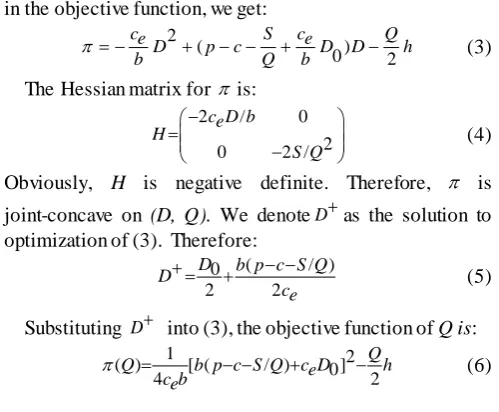
Fig. 5 Trends under situation II

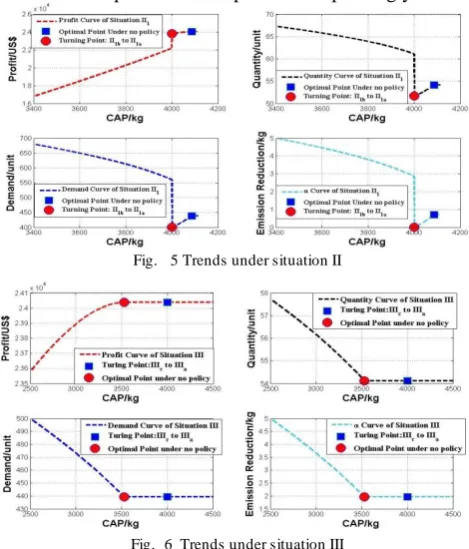
Fig. 6 Trends under situation III

From Figure 5, the curve trends under situation II1 are

shown. It is interesting that before the turning point of sub-situations, the red point, the profit trend is opposite with the others. Since the optimal demand for manufacturer under

Optimal Profit of the Manufacture

no policy is lower than(be_pD₀)/2, decreasing on the lower bound of D under situation II b₁ leads to the decreasing of the optimal demand under carbon cap. After the transferring of sub-situations, the feasible region for D becomes

[D d_{0 1}, ] [d₂,D₀ b e_max], in which the optimal demand lies in d₁. This transferring leads to the cliff-like drop in the figure. As d1increases with CAP, the optimal point finally

reaches its no-policy’s optimal, as shown by the blue point. For Situation III, the trends for all parameters except profit are like the mirror image of that of Situation I, as shown in the figure 6. The increasing on CAP leads to the decreasing ofd₂, the lower bound of D in sub-situationIIc. Optimal demand under carbon cap takes the value of d₂ until d₂ is lower than the optimal demand under no policy, which is the red point shown in the graph. The turning point of sub-situations, therefore, happens in the steady state of the parameters.

In conclusion, under the carbon cap policy, the values of CAP,and m have significant impacts on the manufacturer, shifting the decision situations and the optimal decisions. Lower CAP will limit the optimal profit gain of the manufacturer, vice versa. But the optimal demand, quantity and may shows different trends under different situations. C. Numerical Study on Model under Carbon Tax

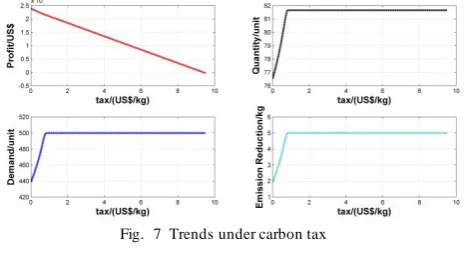
Based on our discussion in previous section, the properties for the carbon tax policy and the carbon cap-and-trade policy are similar under this model. Therefore we only conduct experiments for carbon tax policy, aiming to test when tax rate varies, how firm will make reactions. The basic setting for this experiment is the same as the benchmark problem.

From Figure 7, it is obvious that when the tax rate increases, the profit declines almost linearly, while the quantity, demand and emission reduction amount increase to their maximal values. When the tax rate is up to about 1US$/kg, the manufacturer has to make the most investment to reduce the extra cost incurred by carbon tax.

Fig. 7 Trends under carbon tax

IV. CONCLUSION

In this paper, we propose an EOQ-based model for making joint decisions on production quantity and low-carbon investment. We characterize carbon emission as the total lifecycle emission of a product, and the emission reduction measure is to invest in clean energy and green raw materials, which would likely increase the production cost. Three kinds of carbon policies, namely carbon cap, carbon tax and carbon cap-and-trade, are considered in the proposed model.

We analyze the concavity properties of the proposed model and the situations in which the manufacturer can

profitably make low-carbon investment. The impacts of the three carbon policies are analyzed, and how the optimal value changes with the carbon policies is discussed. Analytical solution processes for the benchmark model and model under the three carbon policies are proposed.

Numerical studies are conducted to reveal that investment in emission reduction can be profitable in low-carbon sensitive markets. The trends of profit, quantity, demand, and emission reduction of the model in different situations under the carbon cap policy are also illustrated.

It is also revealed that manufacturers under carbon cap policies may choose to overproduce to optimize their profits, which may violate the original expectation of policy makers, while manufacturers under carbon tax will choose to increase its quantity and carbon emission investment to lower the cost from carbon tax.

Overall, the numerical studies validate that the proposed model can provide illustrative guidance for making joint decisions to react to different kinds of policies and market situations.

Nevertheless, there are some limitations in the proposed model, which should be addressed in future development. For example, it would be worthwhile to extend the current model to be multi-product and multi-stage, as well as to incorporate more practical issues, such as demand uncertainties, to better satisfy market needs. Moreover, to further combine the view from policy maker can help generate a comprehensive understanding for the carbon policies.

REFERENCE

[1] C2es.org. (2015, 18 DEC. 2015). Industrial Overview | Center for

Climate and Energy Solutions. Available:

http://www.c2es.org/energy/use/industrial

[2] C. Ca rbon Trust, "Product carbon footprinting: the new business opportunity," The Carbon Trust, London, 2008.

[3] S. O'Connell and M. Stutz, "Product carbon footprint (PCF) assessment of Dell laptop-Results and recommendations," in Sustainable Systems

and Technology (ISSST), 2010 IEEE International Symposium on, 2010,

pp. 1-6.

[4] G. Ed wards-Jones, K. Plassmann, E. Yo rk, B. Hounsome, D. Jones, and L. M. i Cana ls, " Vulnerability of e xport ing nations to the development of a carbon label in the United Kingdom," environmental science & policy,

vol. 12, pp. 479-490, 2009.

[5] R. Kirchain, E. Olivetti, T. R. M ille r, and S. Greene, "Sustainable Apparel Materials," 2015.

[6] Solarce llcentra l.co m. (2015, 19 DEC.). Solar Electricity Cost vs.

Regular Electricity Cost. Available:

http://solarcellcentral.com/cost_page.html

[7] S. Ba ldwin, "Ca rbon footprint of electricity generation," London:

Parliamentary Office of Science and Technology, 2006.

[8] E.H. Kim and T. P. Lyon, "When does institutional investor activism pay? The Carbon Disclosure Project," Unpublished Work ing Paper,

2007.

[9] A. Toptal, H. Özlü, and D. Konur, "Joint decisions on inventory replenishment and e mission reduction investment under different emission regulations," International Journal of Production Research,

vol. 52, pp. 243-269, 2014.

[10]S. Zanoni, L. Ma zzoldi, L. E. Zavanella, and M. Y. Jaber, "A jo int economic lot size model with price and environ mentally sensitive demand," Production & Manufacturing Research, vol. 2, pp. 341-354, 2014.

[11]D. Ghosh and J. Shah, "A co mparative analysis of green ing polic ies across supply chain structures," International Journal of Production Economics, vol. 135, pp. 568-583, 2012.

[12]D. Battin i, A. Persona, and F. Sgarbossa, "A Sustainable EOQ Model: theoretical formu lation and applications," International Journal of

Production Economics, vol. 149, pp. 145-153, 2014.