RESEARCH ARTICLE
Can human experts predict solubility
better than computers?
Samuel Boobier
1, Anne Osbourn
2and John B. O. Mitchell
1*Abstract
In this study, we design and carry out a survey, asking human experts to predict the aqueous solubility of druglike organic compounds. We investigate whether these experts, drawn largely from the pharmaceutical industry and academia, can match or exceed the predictive power of algorithms. Alongside this, we implement 10 typical machine learning algorithms on the same dataset. The best algorithm, a variety of neural network known as a multi-layer perceptron, gave an RMSE of 0.985 log S units and an R2 of 0.706. We would not have predicted the relative success of this particular algorithm in advance. We found that the best individual human predictor generated an almost identi-cal prediction quality with an RMSE of 0.942 log S units and an R2 of 0.723. The collection of algorithms contained a higher proportion of reasonably good predictors, nine out of ten compared with around half of the humans. We found that, for either humans or algorithms, combining individual predictions into a consensus predictor by taking their median generated excellent predictivity. While our consensus human predictor achieved very slightly better headline figures on various statistical measures, the difference between it and the consensus machine learning pre-dictor was both small and statistically insignificant. We conclude that human experts can predict the aqueous solubil-ity of druglike molecules essentially equally well as machine learning algorithms. We find that, for either humans or algorithms, combining individual predictions into a consensus predictor by taking their median is a powerful way of benefitting from the wisdom of crowds.
© The Author(s) 2017. This article is distributed under the terms of the Creative Commons Attribution 4.0 International License (http://creativecommons.org/licenses/by/4.0/), which permits unrestricted use, distribution, and reproduction in any medium, provided you give appropriate credit to the original author(s) and the source, provide a link to the Creative Commons license, and indicate if changes were made. The Creative Commons Public Domain Dedication waiver (http://creativecommons.org/ publicdomain/zero/1.0/) applies to the data made available in this article, unless otherwise stated.
Background
Solubility is the property of a chemical solute dissolving in a solvent to form a homogeneous system [1]. Solubility depends on the solvent used, as well as the pressure and temperature at which it was recorded. Water solubility is one of the key requirements of drugs, ensuring that they can be absorbed through the stomach lining and small intestine, eventually passing through the liver into the bloodstream. This means that low solubility is linked with poor bioavailability [2]. Another typical requirement of a drug is delivery in tablet form, again adequate solubility is needed. Tablets are strongly preferred to intravenous delivery of drugs, not least for patient compliance, ease of controlling the dose, and of self-administration. There are also toxicity problems associated with low solubility
drugs, for example crystalluria caused by the drug form-ing a crystalline solid in the body [3]. Moreover, poor pharmacokinetics and toxicity are major causes of late stage failure in drug development. In fact 40% of drug failures stem from poor pharmacokinetics [4].
Prediction of key pharmaceutical properties has become increasingly important with the use of high throughput screening (HTS). As HTS has gained popu-larity, drug candidates have had increasingly higher molecular weight and lipophilicity, leading to lower solu-bility which is considered the predominant problem [5]. It is vital that solubility can be understood and predicted, in order to reduce the number of late stage failures due to poor bioavailability. Thus springs the need for ways to accurately predict both solubility and the essential prop-erties, often referred to as ADMET (absorption, distri-bution, metabolism, elimination and toxicity), in which solubility is a key factor. As a way to increase the suc-cess of developing effective medicines, Lipinski’s popular “rule of five” was an empirical analysis of the attributes
Open Access
*Correspondence: [email protected]
of successful drugs, giving guidelines on what makes a good pharmaceutical [2]. He found that effective drugs had molecular weight < 500, lipophilicity of log P < 5, and numbers of hydrogen bond donor and acceptor atoms that were < 5 and < 10 respectively. Increasingly, in silico approaches are being used to predict ADMET properties, in order to streamline the number of candidates coming through HTS.
Solubility itself is difficult to measure. Typically log S, the base 10 logarithm of the solubility as referred to units of mol/dm3, is reported. There are many different definitions of solubility and various experimental ways of measuring it, which can lead to poor reproducibility of solubility measurements. Thus with varied sources of data, especially when the exact details of the solubility methodology are not specified, assembling a high quality dataset for solubility prediction can be difficult. Thermo-dynamic solubility is the solubility measured under equi-librium conditions. It can be determined with a shake flask approach, or by using a method like CheqSol [6], where equilibration is speeded up by shuttling between super- and subsaturated solutions via additions of small titres of acid or alkali. The Solubility Challenge [7, 8] used its own bespoke dataset, measuring intrinsic aqueous thermodynamic solubility with the CheqSol method. Its authors reported high reproducibility and claimed ran-dom errors of only 0.05 log S units. Despite this, study of the literature suggests that overall errors in reported intrinsic solubilities of drug-like molecules are around 0.6–0.7 log S units, as discussed by Palmer & Mitchell and previously by Jorgensen & Duffy [9, 10].
This means that the best computational predictions possible would have root mean squared errors (RMSE) similar to the experimental error in reported solubilities. The feasible prediction accuracy will be dataset-depend-ent. Using various machine learning (ML) methods simi-lar to those utilised herein, we obtained a best RMSE of 0.69 log S units for a test set of 330 druglike molecules, 0.90 for a different test set of 87 such compounds, 0.91 for the Solubility Challenge test set of 28 molecules, and in the same paper 1.11 log S units for a tenfold cross-val-idation of our DLS-100 set of 100 druglike compounds [11–15]. Further, we define a useful prediction as one with an RMSE smaller than the standard deviation of the experimental solubilities, to avoid being outperformed by the naïve assignment of the mean experimental solubility to all compounds [13].
The use of human participants is widespread in the social sciences, but remains a relatively unused tool in chemistry. This is largely due to the nature of the ques-tions that chemists address. However, human experts are frequently used in surveys about the future of research areas in science, for example asking climate change
experts to respond to a series of statements on the future of the field [16]. Similarly, the results of an expert survey on the future of artificial intelligence were published in 2016 [17].
The wisdom of crowds is the beneficial effect of recruit-ing many independent predictors to solve a problem [18, 19]. Over a 100 years ago, Galton described a competi-tion at a country fair requiring participants to estimate the mass of a cow. Some guesses were large overestimates and others substantial underestimates. Nonetheless, the ensemble of estimates was able to make an accurate pre-diction, as reported in Nature [20]. If some predictors are likely to be very unreliable, then it is better to use the median estimate as the chosen prediction, avoiding the potentially excessive effect of a few ridiculous guesses on the mean [21]. In cheminformatics, the same kind of idea was exploited by Bhat et al. [22] to predict melting points, employing an ensemble of artificial neural net-works rather than a crowd of humans. They reported a large improvement in accuracy, with the ensemble pre-diction being better than even the best performing single neural network. The use of multiple independent models is also fundamental to other ensemble predictors, such as Random Forest, and to consensus methods for rescoring docked protein–ligand complexes [23]. Utilising the wis-dom of crowds requires an algorithm or experiment that can produce many independent predictors, though based on essentially the same pool of input data.
To our knowledge, there has only been one other recent study that has used human experts to solve chemical problems. Orphan drugs are potential pharmaceuticals that remain commercially undeveloped, often because they treat diseases too rare for commercially viable drug development by pharmaceutical companies in a competi-tive market. Regulators incentivise the development of these drugs by allowing market exclusivity; a new drug for these conditions is only approved if is judged to be sufficiently dissimilar to products already on the mar-ket. Judging whether or not two compounds are similar is time consuming for the team of experts. Thus, Franco et al. [24] asked whether computers could reproduce the rulings of experts. Human specialists were shown 100 pairs of molecules and asked to quantify their similar-ity. Their results were statistically compared to similari-ties computed with 2D fingerprint methods. The authors concluded that 2D fingerprint methods “can provide useful information” to regulatory authorities for judging molecular similarity.
consistently using the CheqSol method [6]. The research community was then asked to submit predictions of the aqueous solubilities of 32 further compounds, which had been measured in-house, but were unreported. The subsequently reported results of the Challenge gave a measure of the state of the art in solubility prediction [8]. Nonetheless, the outcome of this blind challenge would have been more interesting and of greater utility had par-ticipants been asked to provide details of the computa-tional methods, and of any experimental data beyond the training set, they used in their predictions.
Machine learning is a subset of Artificial Intelligence (AI), where models can change when exposed to new data [25]. In general, one can use the properties of a large training set to predict the properties of a typically smaller test set. Machine learning has found an array of applications from image recognition and intrusion detec-tion to commercial use in data mining [26–28]. In chem-istry, the application of machine learning is widespread in drug discovery and it can be used to detect toxicity, predict ADMET properties or derive Structure–Activ-ity Relationships (SAR) [29–34]. Supervised machine learning problems can be divided into classification and regression. In classification models, the property to be predicted is a categorical variable and the prediction is which of these classes a new instance should be assigned to, such as soluble or insoluble. Regression problems deal with predicting continuous variables, for instance log S. In chemical applications of machine learning, the prob-lem generally has two parts: firstly encoding molecular structure in the computer, and secondly finding an algo-rithmic or mathematical way of accurately mapping the encodings of structures to values or categories of the out-put property [21, 35]. The encoding typically consists of molecular descriptors, also known as features or attrib-utes. There are thousands of descriptors in use, ranging from ones derived solely from the chemical structure, such as counts of atoms of each element in the molecule and topological and electronic indices, to experimentally derived quantities like log P or melting point [36].
Methods
Dataset and descriptors
Our dataset is the same set of 100 druglike molecules as used in our group’s previous work, which we call the DLS-100 set [13–15]. We chose this because it is a con-venient set of high quality data for which we have a benchmark of the performance of other computational methods. Approximately two-fifths of the molecules had their solubilities measured with the CheqSol method [7, 8, 37, 38], and the remaining data were obtained from a small number of, so far as we can judge, generally reli-able sources [39–43]. All our data are intrinsic aqueous
solubilities, which correspond to the solubility of the neutral form only, in common with our previous studies of solubility [9, 11–13, 37, 44, 45]. For a few molecules, a somewhat arbitrary choice between slightly different quoted literature solubilities had to be made.
The molecules were split into two groups: 75 in the training set and 25 in the test set. The split was made with the following conditions: no molecule in the test set of the aforementioned Solubility Challenge would be in our test set, in case participants had been involved in the Solubility Challenge; the best known pharmacy drugs, like paracetamol, were placed in the training set; and the least soluble and most soluble single molecules were also placed in the training set to avoid any need for extrapo-lation. After these requirements had been satisfied, the rest of the split was chosen at random. Additional file 1 shows the names and structures of 75 compounds in the training set, their solubilities, and a literature source for the solubility; Additional file 2 does the same for the 25 test set molecules. Additional file 3 contains these data in electronic form (.xlsx), including SMILES.
We use SMILES (Simplified Molecular Input Line Entry System) to represent molecules for data input, with letters and numbers conveniently showing the con-nectivity of each atom, where the hydrogen atoms are not explicitly shown, for example Oc1ccccc1 is phenol [46, 47]. These SMILES strings are then used to compute the molecular descriptors which form the encoding of the molecular structure. For this study, we used exactly the same set of 123 Chemistry Development Kit (CDK) [48] descriptors as previously, re-using files originally obtained in 2012 rather than recalculating descriptors [13]. This ensures comparability with the prior work.
Machine learning
of the output properties of the instances [50]. Minimising this entropy favours trees which group together instances with similar property values at the same leaf node, as is highly desirable in making an accurate prediction.
The Random Forest (RF) machine learning method can be used either for classification or, as in the present work, for regression [51, 52]. RF leverages the wisdom of crowds by using a forest consisting of multiple stochas-tically different trees, each based on separately sampled datasets drawn from a common pool of data. Trees are grown based on recursive partitioning of training data consisting of multiple features for each object, the objects here being compounds. The trees are randomised firstly by being based on separate bootstrap samples of the data pool, samples of N out of N objects chosen with replace-ment. Secondly, trees are also randomised by being per-mitted to use only a stochastically chosen subset of the descriptors determined by a parameter known as mtry, with a new subset of mtry descriptors being chosen at each node as the tree is built. For each node, a Gini-optimal [50] split is chosen, so that data are collected into increasingly homogeneous groups down the tree, and thus the set of molecules assigned to each terminal leaf node will share similar values of the property being predicted. The Random Forest thus has a number ntree of stochastically different trees, each derived from a fresh bootstrap sample of the training data. Such a Random Forest of regression trees can then be used to predict unseen numerical test data, with the predictions from the different trees being amalgamated by using their mean to generate the overall prediction of the forest.
Other tree-based ensemble predictors are also used in this work, and most of the above discussion applies equally to them. Bagging is another tree-based ensem-ble predictor [53]. As explained by Svetnick, Bagging is equivalent to RF with mtry equal to the total number of known descriptors, that is all descriptors are available for optimising the splitting at each node [52]. The Extra Trees (or Extremely randomised Trees) algorithm is also related to RF but a third level of randomisation is intro-duced in the form of the threshold for each decision being selected at random rather than optimised [54].
Ada Boost (Adaptive Boosting) [55] is another ensem-ble method also based, in our usage, on tree classifi-ers. The overall classifier is fitted to the dataset using a sequence of weak learners, which in this implementa-tion are decision trees. The weights of each training set instance are equal to begin with, but with each cycle these weights are adjusted to optimise the classifier in the boosting process. Many such cycles are run and the model increasingly focuses on predicting the difficult cases; these potential outliers have greater influence here than in most other methods. The process by which
the weights are optimised is a kind of linear regression, although the underlying weak learners here are not them-selves linear.
Support Vector Machines (SVM) map data into high dimensional space. Kernel functions, typically non-linear, are used to map the data into a high dimensional feature space [56, 57]. An optimal hyperplane is constructed to separate instances of different classes, or in the current case of regression to play the role of a regression line. Put simply, the chosen hyperplane separates the instances such that the margins between the closest points on each side, called support vectors, are maximised. SVM is very effective for problems with many features to learn from, where the data have high dimensionality, and for sparse data [58].
K nearest neighbours (KNN) is a method for classifica-tion and regression, where the predicclassifica-tion is based on the property values of the closest training data instances [59]. For a test instance, the distance to each training instance in the descriptor space is calculated to identify its nearest neighbours; this is usually the Euclidean distance, though other metrics like the Manhattan distance are also usa-ble. The values of different descriptors should be scaled if their ranges significantly differ. K refers to the number of neighbouring training instances to be considered in the prediction. In classification the prediction is the majority vote of K-nearest neighbours, whereas in regression the mean value of the target property amongst the K neigh-bours is taken.
Artificial Neural Networks (ANN) are inspired by the brain’s use of biological neurons, but are vastly less com-plex [60, 61]. A typical ANN will be simpler and smaller than the minimal 302 neuron brain of the nematode worm C. elegans [62]. The ANN architecture has neurons in both an input layer which receives the initial data and an output layer which relays the prediction of the target variable. Between the input and output layers lies a single hidden layer in the typical architecture, or alternatively multiple hidden layers in the case of Deep Learning. Each connection between neurons carries a weight, these being optimised during the training phase as the network learns how best to connect inputs and outputs. ANNs can suffer from overfitting and learning from noise, espe-cially when the training set is small or varied [63]. The variant of ANN used in this study is a back-propagating Multi-Layer Perceptron (MLP) [64].
be unsuitable for complex, and especially non-linear, problems.
Stochastic Gradient Descent (SGD) is another linear method, structuring the problem as a gradient-descent based minimisation of a loss function describing the pre-diction error. SGD optimises the hyperplane, a multidi-mensional analogue of a regression line, by minimising the loss function to convergence [66].
Survey
The ethical approval from the School of Psychology and Neuroscience Ethics Committee, which acts on behalf of the University of St Andrews Teaching and Research Eth-ics Committee (UTREC), is more fully described under Declarations below. The ethics approval letter can be found in Additional file 4. The design of the survey was carefully planned in advance. The Qualtrics suite of soft-ware was used to create an online survey [67].
A human expert was defined as someone with chem-istry expertise, working or studying in a university or industry. A total of 229 emailed invitations were sent out to identified experts. At the start of the survey, par-ticipants were asked their highest level of education and their current field of employment. A pop up link to a webpage with the training data was available on every screen: http://chemistry.st-andrews.ac.uk/staff/jbom/ group/solubility/.
This is in essence an HTML version of Additional file 1. The training data were displayed in a random order, with their respective log S values. Participants were then shown each molecule in the test set, in a random order. They were then asked to predict the aqueous solubility based on the training data. The molecules were displayed as skeletal formulae, drawn with the program ChemDoo-dle [68]. All molecules were shown at the same resolution. A full copy of the survey can be found in Additional file 5.
Results
Choice of median‑based consensus predictors
Our simple experimental design provides no basis to pick either a best machine learning method or best human predictor before analysing the test set results. Hence, we decided in advance that our consensus machine learn-ing predictor would be based on the median solubility predicted for each molecule amongst the ten algorithms. Similarly, our best human predictor would be based on the median solubility predicted for each molecule amongst the human participants. This selection of ensem-ble models means that we expect both our chosen con-sensus predictors to benefit from the wisdom of crowds [18–20]. We also examine the post hoc best individual machine learning method and best human predictor.
Machine learning algorithms
The ten machine learning algorithms were trained on the training set and run on each of the 25 molecules of the test set to generate the predicted solubility. These com-puted solubilities are shown in Additional file 6; their standard deviation was 1.807 log S units. We assessed each machine learning method in terms of the root mean squared error (RMSE), average absolute error (AAE), coefficient of determination which is the square of the Pearson correlation coefficient (R2), Spearman rank cor-relation coefficient (ρ), and number of correct predictions within a margin of one log S unit (NC). These results are shown in Table 1.
[image:5.595.305.539.514.670.2]The MLP performed best of the machine learning algorithms on RMSE, AAE, R2, and ρ. Its RMSE of 0.985 log S units is encouraging and its R2 of 0.706 is a decent result for this dataset, although the different validation methods mean that comparisons with McDonagh et al. [13] can be no more than semi-quantitative. RF also pro-duces good results, with an RMSE of 1.165, and ranks in the top three individual machine learning predic-tors on all criteria. Alongside the closely related Bag-ging method, RF is one of two algorithms to obtain the highest number of correct predictions, with 20. The ten machine learning predictors spanned a range of RMSE from 0.985 to 1.813 log S units. The worst RMSE came from a single decision tree and was essentially identical to the standard deviation (SD) of the test set solubilities; the remaining nine methods gave prediction RMSE well below the sample SD, and thus fulfilled the usefulness criterion.
Table 1 Statistical measures of the performance of the 10 machine learning algorithms and the median-based machine learning consensus predictor
We assessed each machine learning method in terms of the root mean squared error (RMSE), coefficient of determination—which is the square of the Pearson correlation coefficient (R2), Spearman rank correlation coefficient (ρ), number of correct predictions within a margin of one log S unit (NC), and average absolute error (AAE)
RMSE R2 ρ NC AAE
MLP 0.985 0.706 0.837 19 0.728
RF 1.165 0.583 0.736 20 0.802
Bagging 1.165 0.583 0.726 20 0.803
KNN 1.204 0.540 0.704 15 0.917
ExtraTrees 1.227 0.542 0.728 18 0.837 AdaBoost 1.235 0.545 0.708 19 0.851
PLS 1.265 0.507 0.670 15 0.980
SVM 1.280 0.520 0.694 16 0.925
SGD 1.429 0.577 0.752 11 1.185
Our consensus ensemble median machine learning predictor beat nine of the ten individual algorithms on each of RMSE, AAE, R2 and ρ. However, MLP in fact out-performed it on each of these measures and is post hoc clearly the best ML algorithm. Paired difference t-tests on the prediction errors, described in detail below, show few statistically significant differences in the performance of the ML predictors. The only such instances of signifi-cance are that the consensus predictor is significantly different from PLS and SGD at the 5% level, and MLP is also significantly different from SGD. Machine learning scripts used are given in Additional file 7.
Human predictors
A total of 22 answer sets were received from human par-ticipants, a response rate of 9.6%. Of the parpar-ticipants, four were professional PhD holding scientists working in industry, one PhD engaged in scientific communica-tions, eight PhD holders working as University academics between postdoctoral and professorial level, four current postgraduate students, and five current undergraduate students. Amongst the submissions was a set of predic-tions by a self-identified software developer, each solubil-ity being quoted to five decimal places. We considered that the circumstantial evidence of computer use was sufficiently strong to exclude these predictions from the human predictors. Interestingly, these predictions per-formed almost identically to those from our post hoc best ML method, which was MLP. The software developer’s results achieved a statistically significant performance difference compared with the ML method SGD in the paired difference t-tests. By design, they did not contrib-ute to the ML consensus predictor. The exclusion of the software developer’s predictions from the human expert section of the study left a total of 17 participants who made a prediction for each of the 25 molecules, and four who predicted a subset. These estimated solubilities are shown in Additional file 8.
The two best sets of human responses were from anonymous respondents identified as participants 11 and 7, both recorded as being as PhD holders working in academic research. Participant 11 generated an RMSE of 0.942 log S units and an R2 of 0.723, ranking first by RMSE, R2, NC and AAE amongst the individual partici-pants. This performance included 18 correct predictions, more than any other individual human entrant. Partici-pant 7 achieved an RMSE of 1.187 log S units, an R2 of 0.637, and 17 correct predictions, while also ranking the compounds best with a ρ value of 0.867. The 17 full responses achieved RMSE values spanning a large range from 0.942 to 3.020 log S units. Of these, eight were con-sidered clearly useful with RMSE values well below the sample SD; four were close to the SD, within a range of
± 0.15 units of it; five were beyond this range and con-sidered not to qualify as useful predictors on the usual criterion. Nonetheless, all the complete sets of predic-tions were correct to within one log unit for at least nine molecules.
Our consensus ensemble median-based human predic-tor was constructed by taking the median of all human predictions received for each compound, including those from partial entries. This predictor performed very well, scoring an RMSE of 1.087 and an R2 of 0.632, respec-tively beaten by only one and two individual humans. The median human predictor made 21 correct predictions and achieved an AAE of 0.732 log S units, both better than any individual. Using a paired difference t test meth-odology on the absolute errors of each method, described in detail below, we find that the differences between this consensus predictor and 13 of the 17 human experts are statistically significant at the 5% level. Among the human predictions, 24 of the 136 pairwise comparisons show statistically significant differences at the 5% level. Thus there is substantially more variation in the quality of human predictions than of ML predictions.
Comparison of consensus median‑based machine learning and human predictors
An overall comparison of the median-based consensus ML and human descriptors is given in Table 2. While the consensus human classifier performs slightly bet-ter on each of the five measures, we need to establish whether the difference between the two is statistically significant. To do this, we carry out a paired difference test. For each compound, we consider the absolute error made by the consensus predictors, regardless of whether the predictions were underestimates or overestimates of the true solubility. These are shown in Table 3, with the
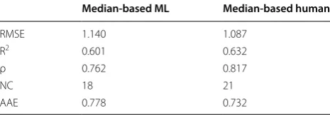
Table 2 Comparison of statistical measures of the perfor-mance of the median-based machine learning consensus predictor and the median-based human consensus predic-tor in terms of the root mean squared error (RMSE), coef-ficient of determination—which is the square of the Pear-son correlation coefficient (R2), Spearman rank correlation
coefficient (ρ), number of correct predictions within a margin of one log S unit (NC), and average absolute error (AAE)
Median‑based ML Median‑based human
RMSE 1.140 1.087
R2 0.601 0.632
ρ 0.762 0.817
NC 18 21
[image:6.595.305.538.643.724.2]difference indicated as positive if the human classifier performs better, and negative if the machine learning one is more accurate for that molecule. The paired difference test seeks to establish whether there is a significant dif-ference in the performance of the two classifiers over the test set of 25 compounds. Thus, we estimate the p value, the probability that so great a difference could arise by chance under the null hypothesis that the two classifiers are of equal quality. Using the data in Table 3, we have carried out both a paired difference t test and also Menke and Martinez’s permutation test [69]. These tests pro-duced p values of 0.576 for the Student’s t test and 0.575 for the permutation test, which show clearly that there is no statistically significant difference between the power of the two classifiers. The relative smallness of a test set containing 25 molecules somewhat limits the statistical
power of such a comparison. However, during testing of the survey we found that predicting solubilities for larger sets of compounds became a long and onerous task, likely to prove beyond the patience of participants. The test set size and methodology is also sufficient to identify significant differences between individual human predic-tors; out of the 153 pairwise t tests amongst these 18 pre-dictors, including the consensus one, 37 are significant at the 5% level.
Comparison of best machine learning and human predictors
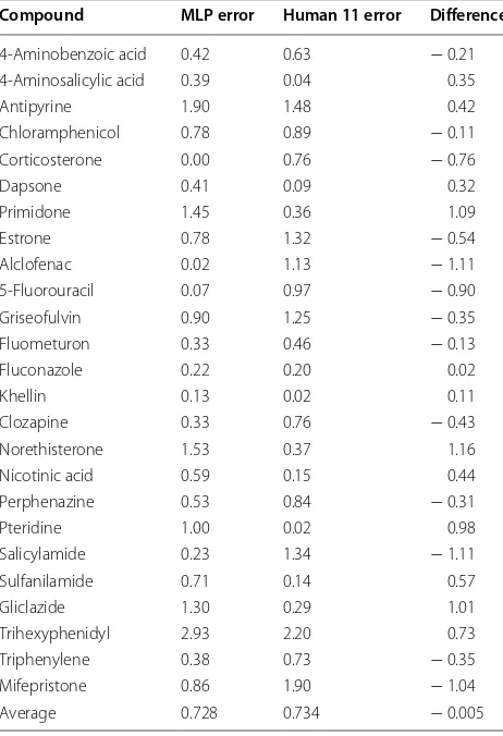
While the identities of the best individual machine learn-ing and human predictors were only known after the fact, it is nonetheless of interest to identify and compare them. Given the nature of the statistical measure we are using, for this comparison we select the individual classifiers with the lowest AAE over the 25 molecules. In each case, these are the same classifiers that have the lowest RMSE and the highest R2, the multi-layer perceptron (MLP) and human participant 11. Their overall performance data are shown in Table 4, with the per-compound comparison in Table 5. The differences are small, though one might observe that the human performs better on three criteria and the perceptron on two.
The statistical significance tests led to p-values of 0.970 for the t-test and 0.969 for the permutation test, indi-cating that there is no statistically significant difference between the power of the two classifiers.
Human predictors: data issues
Possible data input ambiguity
[image:7.595.57.289.123.462.2]Given that 74 out of 75 compounds in the training set and 23 out of 25 in the test set have negative log S values, we expected that the overwhelming majority of predictions would be of negative log S values. Making a prediction of a negative value requires the participant to type a minus sign as part of their input. In fact, a modest number of unexpected individual positive predictions were made. Some of these appear to be clear mistakes; there are three predictions of log S between 4.1 and 6.0 for molecules
Table 3 Performance of median-based consensus clas-sifiers, errors are absolute (unsigned) and are measured in log S units
The difference is meaningfully signed, with a positive value where the human median-based classifier performed better on that compound and a negative value where the machine learning median-based classifier performed better
Compound ML error Human error Difference
4-Aminobenzoic acid 0.07 0.13 − 0.06 4-Aminosalicylic acid 0.23 0.76 − 0.53
Antipyrine 3.73 2.98 0.75
Chloramphenicol 0.35 0.39 − 0.04
Corticosterone 0.11 0.06 0.05
Dapsone 0.54 0.29 0.25
Primidone 0.06 0.14 − 0.08
Estrone 0.87 0.82 0.05
Alclofenac 0.30 0.12 0.18
5-Fluorouracil 0.46 0.62 − 0.16
Griseofulvin 0.44 0.25 0.19
Fluometuron 0.53 0.04 0.49
Fluconazole 1.09 0.70 0.39
Khellin 0.17 0.98 − 0.81
Clozapine 1.37 0.71 0.66
Norethisterone 0.63 0.63 0.00
Nicotinic acid 0.58 0.35 0.23
Perphenazine 0.16 0.16 0.00
Pteridine 2.22 3.02 − 0.80
Salicylamide 0.23 0.49 − 0.26
Sulfanilamide 0.54 0.14 0.40
Gliclazide 1.03 0.80 0.23
Trihexyphenidyl 1.98 1.45 0.53
Triphenylene 0.15 0.27 − 0.12
Mifepristone 1.57 2.00 − 0.43
Average 0.778 0.732 0.046
Table 4 Comparison of statistical measures of the per-formance of the best single machine learning predictor and the best individual human predictor
Multi‑layer perceptron Human participant 11
RMSE 0.985 0.942
R2 0.706 0.723
Spearman ρ 0.837 0.853
Number correct 19 18
[image:7.595.304.539.630.712.2]where the median predictions were between − 3.25 and − 4.5. One human participant subsequently contacted us to report having made at least one sign error. Five other positive valued predictions of log S between 0.2 and 3.2 may or may not be intentional.
While the results analysed above are for the data in their original unedited state, we have also considered the effect of ‘correcting’ for likely data errors. In that analy-sis alone, we have swapped the signs of any predictions of positive log S values where this would reduce the error; this means that all such predictions for compounds with negative experimental log S values had their signs provi-sionally changed.
The principal effect of this change would be to improve some of the weaker human predictors. In this adjusted set of results, the 17 full responses achieved RMSE values spanning a smaller range from 0.942 to 2.313 log S units. Of these, nine were considered clearly useful with RMSE values well below the sample SD; five were within a range
of ± 0.15 units of the SD; three were beyond this range and considered not to be useful predictors on the usual criterion. All the complete sets of human predictions were correct for at least ten molecules. Although the range of prediction quality is reduced, we still note signif-icant differences in predictive power between classifiers even when suspect human predictions are sign-reversed; out of the 153 pairwise t-tests amongst these 18 predic-tors, including the consensus one, 35 are significant at the 5% level.
The median-based approach to constructing our con-sensus classifiers is deliberately designed to be robust to the presence of outlying individual predictions. Although five of the median predictions change slightly upon adjustment of suspect signs, the overall statistics are barely affected with a new RMSE of 1.083, R2 of 0.639, ρ of 0.809, 21 correct predictions, and an AAE of 0.735. The comparison with the consensus machine learning classifier is hardly altered, with a p value from the paired difference t test of 0.600. Since the identity and statistics of the best human classifier are unaffected, the compari-son of the best individual classifiers remains the same under the sign swaps. Thus we note that swapping signs of putative accidental positive log S predictions would have no effect on the main results of this paper, but would improve some of the weaker-performing human classifiers. We do not consider it further.
Data issues in survey training set
At a late stage, it was unfortunately discovered that the data used in the survey training set corresponded to an earlier draft, not the final version, of the solubilities used by McDonagh et al. [13]. There were non-trivial (> 0.25 log S units) differences between the solubility used in the survey training set and the published DLS-100 solubility for six compounds. For sulindac, the DLS-100 solubility is − 4.50 taken from Llinas et al. [7], but the survey train-ing value was − 5.00 from Rytting et al. [39], for L-DOPA, the DLS-100 solubility value is − 1.82 taken from Ryt-ting et al. [39], while the provisional value used in survey training was − 1.12; for sulfadiazine the DLS-100 solubil-ity value is − 3.53 originally taken from Rytting et al. [39], while the value used in survey training was − 2.73; for guanine the DLS-100 solubility is − 4.43 taken from Lli-nas et al. [7], but the survey training value was the − 3.58 from Rytting et al. [39]; for cimetidine the correct DLS-100 solubility is − 1.69 taken from Llinas et al. [7], but an erroneous survey training value of − 3.60 was used. For the remaining 70 training set molecules, the DLS-100 and survey training set solubilities are either identical or within 0.25 log S units.
[image:8.595.57.288.113.451.2]While it was not feasible to repeat the survey, it is pos-sible to train the machine learning algorithms on both
Table 5 Performance of best individual classifiers, errors are absolute (unsigned) and are measured in log S units
The difference is meaningfully signed, with a positive value where the best human classifier performed better on that compound and a negative value where the best machine learning classifier performed better
Compound MLP error Human 11 error Difference
4-Aminobenzoic acid 0.42 0.63 − 0.21 4-Aminosalicylic acid 0.39 0.04 0.35
Antipyrine 1.90 1.48 0.42
Chloramphenicol 0.78 0.89 − 0.11 Corticosterone 0.00 0.76 − 0.76
Dapsone 0.41 0.09 0.32
Primidone 1.45 0.36 1.09
Estrone 0.78 1.32 − 0.54
Alclofenac 0.02 1.13 − 1.11
5-Fluorouracil 0.07 0.97 − 0.90
Griseofulvin 0.90 1.25 − 0.35
Fluometuron 0.33 0.46 − 0.13
Fluconazole 0.22 0.20 0.02
Khellin 0.13 0.02 0.11
Clozapine 0.33 0.76 − 0.43
Norethisterone 1.53 0.37 1.16
Nicotinic acid 0.59 0.15 0.44
Perphenazine 0.53 0.84 − 0.31
Pteridine 1.00 0.02 0.98
Salicylamide 0.23 1.34 − 1.11
Sulfanilamide 0.71 0.14 0.57
Gliclazide 1.30 0.29 1.01
Trihexyphenidyl 2.93 2.20 0.73
Triphenylene 0.38 0.73 − 0.35
Mifepristone 0.86 1.90 − 1.04
sets of training data. The main machine learning results reported herein are based on the correct DLS-100 solu-bilities, but we have also explored the effect of using the imprecise provisional data from the survey training. The effects of the machine learning results are small, though strangely the imprecise training data led to very slightly better median machine learning classifier results (RMSE = 1.095, R2 = 0.632). It appears that the data dif-ferences between the survey training set and the DLS-100 set had very little effect on the quality of the machine learning predictions and therefore are unlikely to have had a substantial effect on the human predictions.
Predictions for different compounds
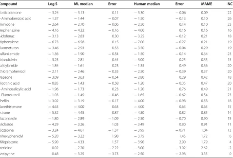
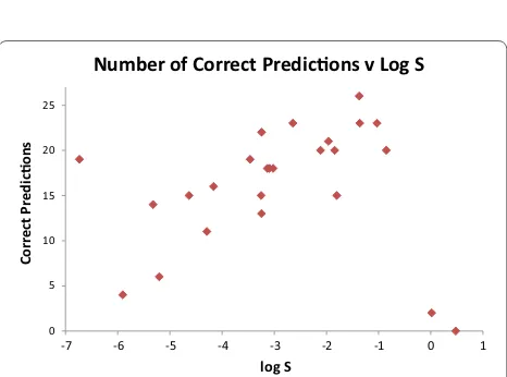
There is a substantial variation in prediction accu-racy between the different molecules in our dataset. In Table 6 below, we rank the 25 compounds by the sizes of the errors from the two consensus predictors. For each compound, we define the average of these two unsigned consensus errors as the Mean Absolute Median Error (MAME), which we display in Fig. 1, and also alongside the number of correct predictions in Table 6. Figure 2
shows the MAME as a function of log S, and Fig. 3 illus-trates how the number of correct predictions varies with solubility. As a general trend, compounds with solubili-ties around the middle of the range are well-predicted. The two most soluble molecules, pteridine and anti-pyrine, are the two worst predicted according to both measures. For the least soluble compounds, the picture is mixed. The second and fourth most insoluble com-pounds, mifepristone and trihexyphenidyl, are poorly handled, being the third and fourth worst predicted on either measure. However, the most insoluble compound, triphenylene, is well predicted and the third most insolu-ble, estrone, moderately well predicted with 14 correct predictions.
As noted before, many compounds have multiple and sometimes significantly different solubility values reported in the literature [9]. There can be confusion between different definitions of solubility, inclusion or exclusion of ionised forms, ambiguity between poly-morphs, systematic differences between experimental methods, kinetic solubility may be wrongly identified as thermodynamic, or the solubility of the wrong compound
Table 6 The 25 test set compounds ranked by the average of the absolute prediction errors of the two consensus predic-tors (mean absolute median error, MAME)
Compound Log S ML median Error Human median Error MAME NC
Corticosterone − 3.24 − 3.13 0.11 − 3.30 − 0.06 0.09 22
4-Aminobenzoic acid − 1.37 − 1.44 − 0.07 − 1.50 − 0.13 0.10 26
Primidone − 2.64 − 2.70 − 0.06 − 2.50 0.14 0.10 23
Perphenazine − 4.16 − 4.32 − 0.16 − 4.00 0.16 0.16 16
Alclofenac − 3.13 − 2.83 0.30 − 3.25 − 0.12 0.21 18
Triphenylene − 6.73 − 6.58 0.15 − 7.00 − 0.27 0.21 19
Fluometuron − 3.46 − 2.93 0.53 − 3.50 − 0.04 0.29 19
Sulfanilamide − 1.36 − 1.90 − 0.54 − 1.50 − 0.14 0.34 23
Griseofulvin − 3.25 − 2.81 0.44 − 3.00 0.25 0.35 15
Salicylamide − 1.84 − 1.61 0.23 − 1.35 0.49 0.36 20
Chloramphenicol − 2.11 − 2.46 − 0.35 − 2.50 − 0.39 0.37 20
Dapsone − 3.09 − 3.63 − 0.54 − 2.80 0.29 0.42 18
Nicotinic acid − 0.85 − 1.43 − 0.58 − 1.20 − 0.35 0.47 20
4-Aminosalicylic acid − 1.96 − 1.73 0.23 − 1.20 0.76 0.49 21
5-Fluorouracil − 1.03 − 1.49 − 0.46 − 1.65 − 0.62 0.54 23
Khellin − 3.02 − 3.19 − 0.17 − 4.00 − 0.98 0.58 18
Norethisterone − 4.63 − 4.00 0.63 − 4.00 0.63 0.63 15
Estrone − 5.32 − 4.45 0.87 − 4.50 0.82 0.85 14
Fluconazole − 1.80 − 2.89 − 1.09 − 2.50 − 0.70 0.90 15
Gliclazide − 4.29 − 3.26 1.03 − 3.49 0.80 0.91 11
Clozapine − 3.24 − 4.61 − 1.37 − 3.95 − 0.71 1.04 13
Trihexyphenidyl − 5.20 − 3.22 1.98 − 3.75 1.45 1.72 6
Mifepristone − 5.90 − 4.33 1.57 − 3.90 2.00 1.79 4
Pteridine 0.02 − 2.20 − 2.22 − 3.00 − 3.02 2.62 2
[image:9.595.60.539.399.724.2]may be measured due to unanticipated chemical reac-tions occurring in the experimental set-up. While we do not claim that poor predictability always implies likely error in the experimental value, this is not unknown. In the Solubility Challenge, indomethacin was very poorly
predicted by computational methods compared to other compounds of similar reported solubility [8]. Subsequent investigation by Comer et al. demonstrated that indo-methacin had undergone hydrolysis during the original CheqSol experiment, and gave a corrected value for its intrinsic solubility [70].
In the distribution of signed errors in the present dataset, only two compounds produce errors (MAME) which lie more than two standard deviations away from the mean; these are antipyrine and pteridine (Fig. 1). For antipyrine, the worst predicted molecule in our dataset, the intrinsic aqueous solubility we used is log S = 0.48, as listed in the dataset curated by Rytting et al. [39] on the basis of earlier work by Herman and Veng-Pedersen [71]. An alternative value of log S = − 0.56 originates from the Aquasol database [72]. Even using this alternative value, antipyrine would still be among the two or three worst predicted compounds in our study. Yalkowsky et al. [73] list seven different room temperature log S values for antipyrine, ranging from − 0.66 to 0.55, their annotations suggesting that they believe the higher solubilities to be more accurate. For pteridine, the solubility of log S = 0.02 was measured by CheqSol and reported in Palmer et al. [37] Two reports from Albert et al. in the 1950’s of sol-ubility of “one part pteridine with 7.2 or 7 parts water” have been translated by Yalkowsky et al. into molar units to give log S = − 0.02 and − 0.03, respectively, and hence barely differ from the CheqSol result [73–75].
Discussion
We have carried out a comparison of consensus pre-dictors from machine learning algorithms and from human experts, the predictors being constructed so as not to require prior selection of the algorithm or human expected to obtain the best results. Comparing over a number of statistical measures of accuracy, we find that there is very little difference in prediction quality between the machine learning and human consensus predictors. While the human median-based predictor obtains slightly better headline figures in all measures, the difference between the two is small and far below
Pteridine Anpyrine
-4.00 -3.00 -2.00 -1.00 0.00 1.00 2.00 3.00
Distribuon of Predicon Error (MAME)
Fig. 1 Per-compound distribution of the average of the absolute prediction errors of the two consensus predictors (Mean Absolute Median Error,
MAME) for the test set. Compounds with errors more than one standard deviation above or below the mean signed error are in orange, those more than two standard deviations away are in red
0.00 0.50 1.00 1.50 2.00 2.50 3.00 3.50 4.00
-7 -6 -5 -4 -3 -2 -1 0 1
Magnitude of erro
r
log S
Magnitude of error (MAME) v Log S
Fig. 2 Magnitude of the average of the absolute prediction errors of
the two consensus predictors (Mean Absolute Median Error, MAME) plotted against experimental log S for the 25 compounds in the test set
0 5 10 15 20 25
-7 -6 -5 -4 -3 -2 -1 0 1
Correct
Predicons
log S
Number of Correct Predicons v Log S
Fig. 3 Number of correct predictions within ± 1 log S unit recorded
[image:10.595.60.540.90.167.2] [image:10.595.58.291.220.381.2] [image:10.595.58.291.433.606.2]statistical significance. We observe that a consensus approach among different machine learning algorithms is likely to be an improvement compared with specifying one particular algorithm in advance, unless one were very confident of which single algorithm to pick. Here, we would not have considered MLP to be our best prospect before seeing the results. A similar conclusion applies to human predictors.
Further, we have carried out a similar comparison of the best machine learning algorithm and the best per-forming human expert. Choosing these as the ‘best’ pre-dictors would have required post hoc knowledge of the results. Here, even the headline result was a virtual tie between the top human and the best algorithm, and there was clearly no significant difference in predictive power.
Both these results lead to the conclusion that machine learning algorithms and human experts predict aqueous solubility essentially equally well. The machine learn-ers had access to over a hundred descriptors for each compound, essentially infallible memory, and the abil-ity to implement intricately designed algorithmic proce-dures with fast and precise numerical calculations. Thus it is perhaps surprising that they were unable to out-perform humans at this task. Our experiences with this study, however, suggest that the prediction of solubility for more than around 25 molecules in one sitting would become an onerous task for most humans, whereas a computer is unlikely to complain if asked to make pre-dictions for a thousand compounds. Thus, our experi-mental design was somewhat contrived to minimise the machines’ inherent advantage of an essentially unlimited attention span.
Even if a human and machine were chess players of equal strength, one might expect that they would cal-culate their best moves in different ways, the human’s experience and understanding versus the machine’s fast, accurate and extensive computation. One might specu-late as to whether or not a similar dichotomy of approach applies here. While we did not ask participants to explain their methods in the survey itself, two experts subse-quently informally reported applying a kind of nearest neighbour algorithm, looking for training set molecules similar to the query compound and then making a judge-ment as to whether the chemical variations between them would increase or decrease solubility. It might seem surprising that a computer could not, with the advan-tages described above, outperform a human at such a task. Nonetheless, human participants in the FoldIt pro-ject have been able to make useful contributions even in a field as apparently computation-intensive as protein fold-ing, at least once the problem was suitably gamified [76]. Perhaps, some of the experts may have been confident
enough in their chemist’s intuition to estimate solubilities without consciously performing an explicit computation. However, our test set was selected to contain relatively unfamiliar compounds to minimise the risk of such a task being performed simply by recall.
A minimally useful prediction has an RMSE very close to the standard deviation of sample solubilities, and can be emulated by the very simple and naïve estimation pro-cedure of computing a mean solubility and then predict-ing this value for every compound. In our experiment, only around half of the humans outperformed this stand-ard. However, nine out of ten machine learners managed this, so the overall machine learning quality is substan-tially better than a minimally useful predictor. Thus, we see no reason to deviate from the fairly well established view that current machine predictors are neither poor enough to fail the usefulness criterion (RMSE around 1.8 log S units in this study), nor good enough for their achievements to be limited only by the uncertainty in experimental solubility data (RMSE approximately 0.6– 0.7) [9]. Machine prediction is currently somewhat bet-ter than the middle of that range, in this study at around an RMSE of 1.0 log S units. Eight machine learning algo-rithms and four human experts, along with both con-sensus predictors, appear superior to a first principles method, which obtained an RMSE of 1.45 on a similar and overlapping, though not identical, set of 25 mole-cules [44]. The latter approach, however, is systematically improvable and provides valuable insight by breaking sol-ubility down to separate sublimation and hydration, and enthalpy and entropy, terms. Considering the best and consensus machine learning and human predictors, these four performed in a range of RMSE of approximately 0.95–1.15, which is numerically slightly better than the machine learning models previously described for the same overall dataset of 100 molecules [13]. However, the different experimental designs and validation strategies preclude direct quantitative comparison. Nonetheless, those individual machine learning approaches common to the two studies, RF, SVM and PLS, gave similar RMSEs to within around ± 0.1 in each case.
However, there were at least two very strong predictors among the humans, competitive with any machine learn-ing approach.
Conclusions
We conclude that human experts can predict aque-ous solubility of druglike molecules essentially equally well as machine learning algorithms. We found that the best human predictor and the best machine learning algorithm, a multi-layer perceptron, gave almost identi-cal prediction quality. We constructed median-based consensus predictors for both human predictions and machine learning ones. While the consensus human pre-dictor achieved very slightly better headline figures on various statistical measures, the difference between it and the consensus machine learning predictor was both small and statistically insignificant. We observe that the collec-tion of machine learning algorithms had a higher propor-tion of useful predictors, nine out of ten compared with around half of the humans. Despite some weak individual human predictors, the wisdom of crowds effect inher-ent in the median-based consensus predictor ensured a high level of accuracy for the ensemble prediction. The best and consensus predictors give RMSEs of approxi-mately 0.95–1.15 log S units, for both machine learning and human experts. Given the estimated uncertainty in available experimental data, the best possible predictors on existing data might achieve RMSEs around 0.6–0.7, though this figure is subject to debate, while a minimally useful predictor would be around 1.8 log S units for our dataset. Thus the current state of prediction, for both humans and machines, is somewhat better than the mid-dle of the range between minimally useful and best realis-tically possible predictors.
Additional files
Additional file 1. The names and structures of 75 compounds in the training set, their solubilities, and a literature source for each solubility value.
Additional file 2. The names and structures of the 25 compounds in the test set, and a literature source for each solubility value.
Additional file 3. The name, structure and solubility data in electronic form for both training and test sets, including SMILES representations of the chemical structures. This DLS-100 dataset may be reused freely with appropriate citation of our work, no further permission is required. It is also available from the University of St Andrews research portal [14] with https://doi.org/10.17630/3a3a5abc-8458-4924-8e6c-b804347605e8 and from figshare [15] with https://doi.org/10.6084/m9.figshare.5545639.
Additional file 4. The ethics approval letter.
Additional file 5. A full copy of the survey given to the human experts.
Additional file 6. The machine learning computed solubility predictions.
Additional file 7. Ten python scripts implementing the different machine learning algorithms.
Additional file 8. The human experts’ solubility predictions.
Authors’ contributions
SB carried out the main body of this research, including the detailed survey design and running the machine learning algorithms, as well as the main analysis of the results. JBOM and AO planned the project. JBOM carried out some further statistical analysis of the results. SB and JBOM co-wrote the final manuscript, parts of which are based on SB’s undergraduate project disserta-tion. All authors read and approved the final manuscript.
Author details
1 Biomedical Sciences Research Complex and EaStCHEM School of Chemistry, University of St Andrews, St Andrews KY16 9ST, Scotland, UK. 2 Department of Met-abolic Biology, John Innes Centre, Norwich Research Park, Norwich NR4 7UH, UK.
Acknowledgements
We thank the anonymous human experts without whom this work would have been impossible.
Competing interests
The authors declare that they have no competing interests.
Availability of data and materials
Additional file 1 shows the names and structures of 75 compounds in the training set, their solubilities, and a literature source for the solubility; Addi-tional file 2 does the same for the 25 test set molecules. Additional file 3 con-tains these data in electronic form, including SMILES. The DLS-100 dataset may be reused freely with appropriate citation of our work, no further permission is required. It is also available from the University of St Andrews research portal [14] with https://doi.org/10.17630/3a3a5abc-8458-4924-8e6c-b804347605e8 and from figshare [15] with https://doi.org/10.6084/m9.figshare.5545639. The ethics approval letter can be found in Additional file 4. A full copy of the survey is in Additional file 5. The computed machine learning solubilities are given in Additional file 6. Machine learning scripts used are given in Additional file 7, which is a .zip file containing ten python scripts. The human experts’ predictions are in Additional file 8.
Consent for publication
All human participants have consented to the use of their non-identifiable data being used in this research, see Additional files 4 and 5. The consent form itself is on the first two pages of Additional file 5. Consent was given online and anonymously, it was not possible to continue the survey beyond the consent request without clicking the “I consent” button.
Ethics approval and consent to participate
Ethical approval was required for this survey, due to its use of human participants. The application was brought before the School of Psychology and Neuroscience Ethics Committee, which acts on behalf of the University of St Andrews Teaching and Research Ethics Committee (UTREC), and was approved on 11th October 2016, with the approval code PS12383. The ethics approval letter can be found in Additional file 4. The key point was ensuring the anonymity of the participants, which was achieved by an anonymous link to the survey, asking only for non-identifying personal information and secure handling and storage of data. Participants were also asked to consent to the use of their data, allowed to leave any answer blank, leave the survey at any point and shown a page of debriefing information at the end of the survey.
Funding
This work took place as SB’s MChem undergraduate research project at the University of St Andrews. We thank University of St Andrews Library for fund-ing the Open Access publication of this work. AO’s laboratory is supported by the UK Biotechnological and Biological Sciences Research Council (BBSRC) Institute Strategic Programme Grant ‘Molecules from Nature’ (BB/P012523/1) and the John Innes Foundation.
Publisher’s Note
Springer Nature remains neutral with regard to jurisdictional claims in pub-lished maps and institutional affiliations.
References
1. Savjani KT, Gajjar AK, Savjani JK (2012) Drug solubility: importance and enhancement techniques. ISRN Pharm 2012:195727. https://doi. org/10.5402/2012/195727
2. Lipinski CA, Lombardo F, Dominy BW, Feeney PJ (2001) Experimental and computational approaches to estimate solubility and permeabil-ity in drug discovery and development settings. Adv Drug Deliv Rev 46(1–3):3–26
3. Simon DI, Brosius FC, Rothstein DM (1990) Sulfadiazine crystalluria revis-ited: the treatment of Toxoplasma encephalitis in patients with acquired immunodeficiency syndrome. Arch Intern Med 150:2379–2384 4. Kennedy T (1997) Managing the drug discovery/development interface.
Drug Discov Today 2:436–444
5. Lipinski C (2002) Poor aqueous solubility—an industry wide problem in drug discovery. Am Pharm Rev 5:82–85
6. Box K, Comer JE, Gravestock T, Stuart M (2009) New ideas about the solubility of drugs. Chem Biodivers 6(11):1767–1788
7. Llinas A, Glen RC, Goodman JM (2008) Solubility challenge: can you predict solubilities of 32 molecules using a database of 100 reliable measurements? J Chem Inf Model 48:1289–1303
8. Hopfinger AJ, Esposito EX, Llinas A, Glen RC, Goodman JM (2008) Find-ings of the challenge to predict aqueous solubility. J Chem Inf Model 49(1):1–5
9. Palmer DS, Mitchell JBO (2014) Is experimental data quality the limiting factor in predicting the aqueous solubility of druglike molecules? Mol Pharm 11(8):2962–2972
10. Jorgensen WL, Duffy EM (2002) Prediction of drug solubility from struc-ture. Adv Drug Deliv Rev 54(3):355–366
11. Palmer DS, O’Boyle NM, Glen RC, Mitchell JBO (2007) Random forest mod-els to predict aqueous solubility. J Chem Inf Model 47(1):150–158 12. Hughes LD, Palmer DS, Nigsch F, Mitchell JBO (2008) Why are some
properties more difficult to predict than others? A study of QSPR models of solubility, melting point, and log P. J Chem Inf Model 48(1):220–232 13. McDonagh JL, Nath N, De Ferrari L, Van Mourik T, Mitchell JBO (2014)
Uniting cheminformatics and chemical theory to predict the intrinsic aqueous solubility of crystalline druglike molecules. J Chem Inf Model 54:844–856. https://doi.org/10.1021/ci4005805
14. Mitchell JBO, McDonagh JL, Boobier S. DLS-100 solubility data-set. University of St Andrews Research Portal. https://doi. org/10.17630/3a3a5abc-8458-4924-8e6c-b804347605e8
15. Mitchell JBO, McDonagh JL, Boobier S. DLS-100 solubility dataset, Fig-share. https://doi.org/10.6084/m9.figshare.5545639
16. Gattuso J-P, Mach KJ, Morgan G (2013) Ocean acidification and its impacts: an expert survey. Clim Change 117:725–738
17. Müller VC, Bostrom N (2016) Fundamental issues of artificial intelligence. Springer, Berlin, pp 553–570
18. Surowiecki J (2004) The wisdom of crowds: why the many are smarter than the few and how collective wisdom shapes business, economies, societies, and nations. Doubleday, New York
19. Iyer R, Graham J (2012) Leveraging the wisdom of crowds in a data-rich utopia. Psychol Inq 23:271–273
20. Galton F (1907) Vox populi. Nature 75:450–451
21. Mitchell JBO (2014) Machine learning methods in chemoinformatics. WIREs Comput Mol Sci 4(5):468–481
22. Bhat AU, Merchant SS, Bhagwat SS (2008) Prediction of melting points of organic compounds using extreme learning machines. Ind Eng Chem Res 47:920–925
23. Charifson PS, Corkery JJ, Murcko MA, Walters WP (1999) Consensus scor-ing: a method for obtaining improved hit rates from docking databases of three-dimensional structures into proteins. J Med Chem 42:5100–5109 24. Franco P, Porta N, Holliday JD, Willett P (2014) The use of 2D fingerprint
methods to support the assessment of structural similarity in orphan drug legislation. J Cheminform 6:5
25. Michalski RS, Carbonell JG, Mitchell TM (2013) Machine learning: an artificial intelligence approach. Springer, Berlin
26. Bishop CM (2006) Pattern recognition and machine learning. Springer, New York
27. Tsai C-F, Hsu Y-F, Lin C-Y, Lin W-Y (2009) Intrusion detection by machine learning: a review. Expert Syst Appl 36:11994–12000
28. Bose I, Mahapatra RK (2001) Business data mining—a machine learning perspective. Inf Manag 39:211–225
29. Burbidge R, Trotter M, Buxton B, Holden S (2001) Drug design by machine learning: support vector machines for pharmaceutical data analysis. Comput Chem 26:5–14
30. Lavecchia A (2015) Machine-learning approaches in drug discovery: methods and applications. Drug Discov Today 20:318–331 31. Judson R, Elloumi F, Setzer RW, Li Z, Shah I (2008) A comparison of
machine learning algorithms for chemical toxicity classification using a simulated multi-scale data model. BMC Bioinform 9:241
32. Cheng F, Li W, Zhou Y, Shen J, Wu Z, Liu G, Lee PW, Tang Y (2012) admet-SAR: a comprehensive source and free tool for assessment of chemical ADMET properties. J Chem Inf Model 52:3099–3105
33. King RD, Muggleton SH, Srinivasan A, Sternberg M (1996) Structure-activity relationships derived by machine learning: the use of atoms and their bond connectivities to predict mutagenicity by inductive logic programming. Proc Natl Acad Sci 93:438–442
34. Reker D, Schneider P, Schneider G (2016) Multi-objective active machine learning rapidly improves structure–activity models and reveals new protein–protein interaction inhibitors. Chem Sci 7:3919–3927 35. Lusci A, Pollastri G, Baldi P (2013) Deep architectures and deep learning
in chemoinformatics: the prediction of aqueous solubility for drug-like molecules. J Chem Inf Model 53:1563–1575
36. Todeschini R, Consonni V (2008) Handbook of molecular descriptors, vol 11. Wiley, London
37. Palmer DS, Llinas A, Morao I, Day GM, Goodman JM, Glen RC et al (2008) Predicting intrinsic aqueous solubility by a thermodynamic cycle. Mol Pharm 5(2):266–279
38. Narasimham LYS, Barhate VD (2011) Kinetic and intrinsic solubility deter-mination of some beta-blockers and antidiabetics by potentiometry. J Pharm Res 4(2):532–536
39. Rytting E, Lentz KA, Chen XQQ, Qian F, Vakatesh S (2005) Aqueous and cosolvent solubility data for drug-like organic compounds. AAPS J 7(1):E78–E105
40. Shareef A, Angove MJ, Wells JD, Johnson BB (2006) Aqueous solubilities of estrone, 17β-estradiol, 17α-ethynylestradiol, and bisphenol A. J Chem Eng Data 51(3):879–881
41. Ran Y, Yalkowsky SH (2001) Prediction of drug solubility by the general solubility equation (GSE). J Chem Inf Comput Sci 41(2):354–357 42. Bergstrom CAS, Luthman K, Artursson P (2004) Accuracy of calculated
pH-dependent aqueous drug solubility. Eur J Pharm Sci 22(5):387–398 43. Bergstrom CAS, Wassvik CM, Norinder U, Luthman K, Artursson P (2004)
Global and local computational models for aqueous solubility prediction of drug-like molecules. J Chem Inf Comput Sci 44(4):1477–1488 44. Palmer DS, McDonagh JL, Mitchell JBO, van Mourik T, Fedorov MV (2012)
First-principles calculation of the intrinsic aqueous solubility of crystalline druglike molecules. J Chem Theory Comput 8(9):3322–3337
45. McDonagh JL, van Mourik T, Mitchell JBO (2015) Predicting melting points of organic molecules: applications to aqueous solubility prediction using the general solubility equation. Mol Inf 34(11–12):715–724 46. Weininger D (1988) SMILES, a chemical language and information system.
1. Introduction to methodology and encoding rules. J Chem Inf Comput Sci 28(1):31–36
47. O’Boyle NM (2012) Towards a universal SMILES representation—a standard method to generate canonical SMILES based on the InChI. J Cheminform 4(1):22
48. Steinbeck C, Han Y, Kuhn S, Horlacher O, Luttmann E, Willighagen E (2003) The chemistry development kit (CDK): an open-source java library for chemo- and bioinformatics. J Chem Inf Comput Sci 43(2):493–500 49. Quinlan JR (1986) Induction of decision trees. Mach Learn 1:81–106 50. Raileanu LE, Stoffel K (2004) Theoretical comparison between the Gini
index and information gain criteria. Ann Math Artif Intell 41:77–93 51. Breiman L (2001) Random forests. Mach Learn 45:5–32
52. Svetnik V, Liaw A, Tong C, Culberson JC, Sheridan RP, Feuston BP (2003) Random forest: a classification and regression tool for compound clas-sification and QSAR modeling. J Chem Inf Comput Sci 43:1947–1958 53. Breiman L (1996) Bagging predictors. Mach Learn 24:123–140 54. Geurts P, Ernst D, Wehenkel L (2006) Extremely randomized trees. Mach
Learn 63:3–42
55. Schapire RE (2003) Nonlinear estimation and classification. Springer, Berlin, pp 149–171
57. Schölkopf B, Smola A (2005) Support vector machines. In: Encyclopedia of biostatistics. Wiley. http://dx.doi.org/10.1002/0470011815.b2a14038 58. Garreta R, Moncecchi G (2013) Learning scikit-learn: machine learning in
python. Packt Publishing Ltd, Birmingham, pp 25–27
59. Denoeux T (1995) A k-nearest neighbor classification rule based on Dempster–Shafer theory. IEEE Trans Syst Man Cybern 25:804–813 60. Hopfield JJ (1988) Artificial neural networks. IEEE Circuits Devices Mag
4:3–10
61. Pham DT, Packianather M, Afify A (2007) Computational intelligence. Springer, Berlin, pp 67–92
62. Connors BW, Long MA (2004) Electrical synapses in the mammalian brain. Annu Rev Neurosci 27:393–418
63. Hinton GE, Srivastava N, Krizhevsky A, Sutskever I, Salakhutdinov RR (2012) ArXiv Preprint http://arxiv.org/abs/1207.0580, pp 1–18 64. Collobert R, Bengio S (2004) Links between perceptrons, MLPs and
SVMs. In: Proceedings of the twenty-first international conference on machine learning. ICML ‘04. New York, NY, USA. ACM. https://doi. org/10.1145/1015330.1015415
65. Wold S, Sjostrom M, Eriksson L (2001) PLS-regression: a basic tool of chemometrics. Chemom Intell Lab Syst 58(2):109–130
66. Bottou L (2010) Proceedings of COMPSTAT’2010. Springer, Berlin, pp 177–186
67. Qualtrics (Version Feb 2017), Provo, Utah, USA, 2017. http://www.qual-trics.com
68. ChemDoodle (Version 8.1.0), iChemLabs, 2017. https://www.chemdoo-dle.com
69. Menke J, Martinez TR (2004) Using permutations instead of student’s t distribution for p-values in paired-difference algorithm comparisons. In: 2004 IEEE international joint conference on neural networks (IEEE Cat. No. 04CH37541). IEEE, pp 1331–1335. https://doi.org/10.1109/ ijcnn.2004.1380138
70. Comer J, Judge S, Matthews D, Towers L, Falcone B, Goodman J et al (2014) The intrinsic aqueous solubility of indomethacin. ADMET DMPK. https://doi.org/10.5599/admet.2.1.33
71. Herman RA, Veng-Pedersen P (1994) Quantitative structure–pharmacoki-netic relationships for systemic drug distribution kistructure–pharmacoki-netics not confined to a congeneric series. J Pharm Sci 83(3):423–428
72. Yalkowsky SH, Dannenfelser RM (1992) Aquasol database of aqueous solubility. College of Pharmacy, University of Arizona, Tucson 73. Yalkowsky SH, He Y, Jain P (2010) Handbook of aqueous solubility data.
CRC Press, Boca Raton
74. Albert A, Brown DJ, Cheeseman G (1951) 103. Pteridine studies. Part I. Pteridine, and 2- and 4-amino- and 2- and 4-hydroxy-pteridines. J Chem Soc 474–485. http://doi.org/10.1039/JR9510000474
75. Albert A, Lister JH, Pedersen C (1956) 886. Pteridine studies. Part X. Pteridines with more than one hydroxy- or amino-group. J Chem Soc 4621–4628. http://doi.org/10.1039/JR9560004621