Contrasting singleton type 1 and interval type 2 non singleton type 1 fuzzy logic systems

Contrasting Singleton Type-1 and Interval Type-2 Non-singleton

Type-1 Fuzzy Logic Systems

Jabran Hussain Aladi,

Student Member, IEEE,

Christian Wagner,

Senior Member, IEEE,

Amir Pourabdollah,

Member, IEEE

and Jonathan M. Garibaldi,

Member, IEEE,

Abstract—Most applications of both type-1 and type-2 fuzzy logic systems are employing singleton fuzzification due to its simplicity and reduction in its computational speed. However, using singleton fuzzification assumes that the input data (i.e., measurements) are precise with no uncertainty associated with them. This paper explores the potential of combining the uncer-tainty modelling capacity of interval type-2 fuzzy sets with the simplicity of type-1 fuzzy logic systems (FLSs) by using interval type-2 fuzzy sets solely as part of the non-singleton input fuzzifier. This paper builds on previous work and uses the methodological design of the footprint of uncertainty (FOU) of interval type-2 fuzzy sets for given levels of uncertainty. We provide a detailed investigation into the ability of both types of fuzzy sets (type-1 and interval type-2) to capture and model different levels of uncertainty/noise through varying the size of the FOU of the underlying input fuzzy sets from type-1 fuzzy sets to very “wide” interval type-2 fuzzy sets as part of type-1 non-singleton FLSs using interval type-2 input fuzzy sets. By applying the study in the context of chaotic time-series prediction, we show how, as uncertainty/noise increases, interval type-2 input fuzzy sets with FOUs of increasing size become more and more viable.

I. INTRODUCTION

Uncertainty exists in almost all real life applications and their performance can be affected when facing high level of uncertainties. Therefore, it is crucial for these application systems to have the ability to handle these uncertainties. Fuzzy sets (FSs) and fuzzy logic systems (FLSs) are established con-cepts and techniques that have been accepted as methodologies for building systems that can deliver excellent performance in the face of uncertainty and imprecision [1]–[4]. There are many sources of uncertainty facing FLSs such as the presence of noise in the training data, the noise affecting inputs and outputs and the linguistic uncertainty associated with the linguistic terms in the antecedents of the rule base [5] [6].

Non-singleton fuzzy logic systems (NSFLSs) [7] [8] were introduced to model the uncertainty of input signals as an extension to singleton fuzzy logic systems (SFLSs) which are not adequate when input data is corrupted by measurement noise [9]. In NSFLSs, the inputs are modelled as fuzzy sets and are no longer as crisp values. NSFLSs have been used successfully in a variety of applications [10]–[23] and new advancements in developing new types of NSFLS have shown superior results (e.g., in [24]).

The authors are with the Lab for Uncertainty in Data and Decision Making (LUCID), School of Computer Science, University of Nottingham, Nottingham, UK. (E-mails: [email protected], [email protected], [email protected], [email protected].)

The modelling processes of various sources of uncertainties in NSFLSs can be systematically achieved as follows:

• The input uncertainties of an FLS are modelled using input FSs, for example the uncertainties from the sensor readings that provide the inputs to an FLS.

• The control output uncertainties of an FLS are modelled using output FSs. These result for example from the changes in the actuators or motor characteristics due to environmental conditions.

• The uncertainties in linguistic labels which are the am-biguity in the meanings of the words used to label the antecedents and the consequent FSs used in fuzzy logic rules, for example the labels ‘left’ or ‘fast’.

From the above step-by-step uncertainty modelling ap-proach, it can be recognised that, the input uncertainties are modelled using input FSs (in case of NSFLSs) then they are combined with antecedent FSs that are used to model the uncertainties of the linguistic labels for the inputs in the fuzzy rules. In this process, the input uncertainties are modelled separately from the uncertainties of antecedent terms and then combined afterwards.

However, in our previous works [25], [26], the modelling of uncertainty affecting the FLS inputs is conducted as part of the antecedent FSs. In principle however, established FLS method-ology foresees the use of the input FSs for the modelling of input uncertainty while antecedent FSs model uncertainty in the linguistic antecedent terms. While in most singleton FLS applications, uncertainty in input and antecedent terms is “mixed” in the antecedent FSs, for the step-by-step modelling approach put forward in [25], exploring the application with a non-singleton fuzzification approach would be highly valuable. In such an approach, the proposed methodology in [25] to determine an appropriate footprint of uncertainty (FOU) for the antecedent FSs would be adjusted in this paper to generate appropriate FOUs for the input FSs based on input uncertain-ties, achieving potentially a more efficient FLS design.

In this paper, we use the application domain of time series prediction (TSP) to investigate the performance of the different generated type-1 fuzzy logic systems (T1 FLSs) with different input fuzzy sets by transitioning from inputs employing type-1 fuzzy sets (Ttype-1 FSs) to inputs employing interval type-2 fuzzy sets (IT2 FSs) with varying sizes of FOU in the face of different inputs with varying signal-to-noise ratios (SNRs).

singletonbFS T1bnon-singletonbbFSb whenbFOUbsizebcb=0

IT2bnon-singletonbbFSsb whenbFOUbsizesbcb>b0

InputbT1bFSs OutputbT1bFSs

CrispbInput

CrispbOutput Fuzzifier Rulebase Defuzzifier

InferencebEngine

x' x' x' x' x'

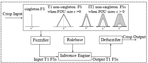
Fig. 1. The structure of the singleton and the type-1/interval type-2 non-singleton type-1 FLS

used to obtain an input IT2 FS of a given size around an input T1 FS with a constant FOU size over the ‘core’ of the input FS. This approach enables the transition from input T1 FSs to input IT2 FSs while maintaining a desired level of uncertainty in the primary memberships of the resulting input IT2 FSs over the domain of the lower MF of the input IT2 FS. It is worth noting that the main objective of this paper is not to achieve optimal performance in a given application such as TSP, but to explore the transitioning from input T1 to input IT2 FSs by selecting the optimal FOU size for given levels of uncertainty/noise.

The rest of the paper is structured as follows. In Section II, a review of Non-singleton fuzzy logic system (NSFLS) and FOU creation method are provided. The proposed approach is applied to Mackey-Glass time series prediction and presented in Section III. The results of the study are presented and discussed in Section IV. The conclusion and future work appear in Section V.

II. BACKGROUND

This section provides a brief overview of the concepts used later in the paper. These concepts include singleton and non-singleton FLS and the FOU creation method with their use in different fuzzification types.

A. Singleton and Non-singleton Type-1 Fuzzy Logic System

According to the type of fuzzification [14], T1 FLSs can be divided into singleton fuzzy logic system (SFLS) and non-singleton fuzzy logic system (NSFLS), which are presented below. T1 FLS (as shown in Fig. 1) is described by T1 FSs and consists of four components, which are the fuzzifier, the rule base, the inference engine and the defuzzifier [14].

In singleton T1 FLS, crisp inputs are first fuzzified, usually into input T1 FSs. These activate the inference engine and the rule base to produce output T1 FSs which are then combined to produce an aggregated T1 output FSs. The defuzzifier finally defuzzifies the aggregated T1 fuzzy outputs to produce crisp outputs. Further detail on SFLSs can be found for example in [12] [14].

A T1 FLS whose inputs are modelled as T1/IT2 FSs is referred to as ‘T1/IT2 singleton T1 FLS’. A T1/IT2 non-singleton T1 FLS has the same structure as a non-singleton T1 FLS, see Fig. 1, and they share the same type of rules; the

0.0

1.0

a δ x' δ b a x' b

0.0

1.0

FOU creation

metod c=0.5

T1 MF UMF

LMF

(a) (b)

c

T1 MF

Fig. 2. Illustration example of the FOU creation of IT2 MF by transitioning from (a) initial T1 FS to (b) IT2 FS obtained using FOU size parameter

c= 0.5.

major difference is the type of fuzzification. The majority of FLSs are using SFLS because the singleton fuzzification is simpler and faster to compute. In singleton fuzzification, inputs are considered to be singleton FSs, while the non-singleton fuzzification models the FLS inputs as FSs. More details on NSFLSs can be found for example in [12], [14], [20].

B. FOU Creation Method to represent the Input Value

As previously introduced in [25], this method is used to obtain an IT2 FSs with a uniform (constant) FOU over the ‘core’ of the FS. This method based on a fixed parametercthat is used to create an FOU of a given size around a principal (T1) MF. In order to create the IT2 FSs based on the uncertainty parameter c and the T1 MF, we employ (1) and (2) shown below to create the resulting upper membership function (UMF) and lower membership function (LMF) respectively.

µ_xi(xi) = min

µxi(xi) +

c 2,1.0

(1)

µ

xi(xi) = min

maxµxi(xi)−

c 2,0

,1.0−c, (2)

whereµxi(xi)relates to the T1 MFs such as the triangular FS

shown in (4) andcis the FOU size parameter. For more details on this method we refer the reader to [25]. A more detailed illustration of the FOU design of the IT2 FS is depicted in Fig. 2. In Fig. 2(a) the possible range which the triangular T1 MF center (mean) can vary is considered to be ±δ (will be detailed in II-B2)

1) Singleton Type-1 FLS with Singleton Fuzzy Sets to

Represent the Input Value: In singleton T1 FLS, the fuzzifier

converts the crisp inputs into linguistic terms with given membership value to activate the rule base and inference engine. The fuzzification between singleton fuzzy input and antecedent T1 FS to obtain the membership values of inputi

within rulercan be found as follows:

µr_i(xi) =µ_{F i} r

(xi), (3)

wherexiis theithinput value andµ_{F i} r

(xi)is the membership

2) Type-1 Non-Singleton Type-1 FLS with Triangular Fuzzy

Sets to Represent the Input Value: In type-1 non-singleton

type-1 FLSs, the fuzzy inputs can be modelled using triangular, Gaussian or any other MF shape. The considered non-singleton fuzzy inputs employ triangular MF, and are centred at the given input value. The spread of the FS is related to the amount of uncertainty facing the FLS (e.g., the additive noise standard deviation). In our case the possible range which each triangular center (mean) can vary is considered to be ±δ, where δ is related to the additive noise standard deviation.

The membership value of the triangular T1 fuzzy inputs in a T1 non-singleton type-1 FLS can be written as:

µxi(xi) =

    

   

0 xi≤a

xi−a x0

i−a

a≤xi≤x0i b−xi

b−x0

i

x0_i≤xi≤b

0 xi≥b

, (4)

where, xi is the ith input value, x0i is the input value, a =

(x0_i−δ) is the left endpoint, and b = (x0_i+δ) is the right endpoint.

The fuzzifier converts the fuzzy input into linguistic terms with given membership value to activate the rule base and inference engine. The composition between type-1 fuzzy input and antecedent T1 FS to obtain the membership values of input

i within rulercan be found as follows:

µri(xi) = sup xi∈Xi

(µxi(xi)∗µF i_r(xi)), (5)

whereµxi(xi)is the membership value of the T1 fuzzy input

andµ

F i_r(xi)is the membership value of the antecedent T1 FS.

In this paper, the ‘sup’ operation is considered to be maximum t-conorm and the * operation is considered to be the product. The antecedent/consequent type-1 fuzzy sets are shown in Fig. 3 whereas the triangular type-1 fuzzy input whenx0_iis theith

input value is shown in Fig. 2 (a).

3) Interval Type-2 Non-Singleton Type-1 FLS with

Triangu-lar Fuzzy Sets to Represent the Input Value: In the literature

considering the application of IT2 FLSs, the mostly considered are the use of singleton T2 FLSs in which the inputs are crisp values. Also, few papers considered the use of T2 non-singleton T2 FLSs [14]–[17] where the uncertainty in inputs are modelled using type-2 fuzzy inputs. However, to the best of our knowledge, no work presented so far considering the use of IT2 non-singleton T1 FLSs where the uncertainty in inputs to a T1 FLS are modelled using IT2 fuzzy inputs. The later approach as well as the previous two (in subsections II-B1 and II-B2) will be adopted in this paper.

Our previous work in [25] (summarised above in Section II-B) is adjusted to be used here to generate appropriate FOUs for the input FSs based on input uncertainty. In order to create the IT2 version of each initial T1 set, the FOU size is specified using the parameter c ∈ [0,1]. Note thatc = 0 results in an input T1 FS with the original MF whilec= 1.0 results in an input IT2 set with a very wide FOU.

0 .0 0 .5 1 .0 1 .5

0

.0

1

.0

u

F1 F2 F3 F4 F5 F6 F7

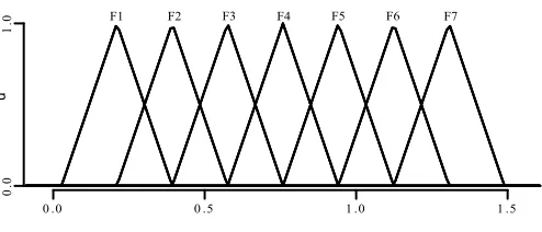
Fig. 3. The antecedent/consequent type-1 fuzzy sets

The upper membership value of the IT2 fuzzy inputµ_xi(xi)

and the lower membership value of the IT2 fuzzy inputµ

xi(xi)

can be obtained from (1) and (2) respectively.

The composition between IT2 fuzzy input and the an-tecedent T1 FS for finding the upper and lower membership values of input i within rule r can be obtained using the following equations, (6) and (7) respectively.

µr_i(xi) = sup xi∈Xi

(µ_xi(xi)∗µ_{F i} r

(xi)), (6)

µr

i(xi) = sup xi∈Xi

(µ

xi(xi)∗µF i_r(xi)), (7)

whereµr_i(xi)andµr_i(xi)are the upper and lower membership

values of fuzzy input, and µ

F i_r(xi) is the membership value

of the antecedent T1 FS. In this paper, the ‘sup’ operation is considered to be maximum t-conorm and the * operation is considered to be the product. The antecedent/consequent type-1 fuzzy sets are shown in Fig. 3 whereas the IT2 fuzzy input when x0_i is the ith _{input value is shown in Fig. 2(b).}

After considering the proposed FOU creation technique for input fuzzy sets and their fuzzification process, we proceed to an experimental exploration of the different behaviour of IT2 input FSs created using FOU creation method when transitioning from an input T1 to an input IT2 FS.

III. EXPERIMENTSMETHODOLOGY ANDRESULTS

A. Experimental Data

1) Mackey-Glass Time Series: FLSs have been successfully

used in forecasting of time series [14], [27]–[29]. As the level of noise/uncertainty is easily controllable, we use time-series prediction here as a testbed to explore the different approaches to IT2 FLS generation. We use the Mackey-Glass (MG) time series which is a chaotic time series proposed in [30]. It is a first-order differential-delay equation originally used to model physiological systems. It is generated from the following non-linear differential equation:

dx(t) dt =

a∗x(t−τ)

1 +xn_(t−τ)−b∗x(t) (8)

used in this paper with the following parameters: a = 0.2,

b= 0.1,τ = 30andn= 10and solved using Euler’s method [31] with a step size equal to 1.0. The initial values of x(t)

for all values of t≤τ are set to 0.9.

2) Additive Noise: To make the prediction more

challeng-ing, noise can be added to the time series. The level of noise is commonly measured by the SNR where a high SNR refers to a more clear signal (low noise) and a low SNR refers to a more noisy signal (high amount of noise). The formula for the SNR (in dBs) [14] is:

SNR (in dBs) = 10∗log₁₀ (σ

2 signal

σ2 noise

), (9)

whereσ2

signal is the variance of the signal andσ2noise is the variance of the noise. To find σnoise, we solve (9) for σnoise as, i.e.:

σnoise =

σsignal

10(SNR20 )

(10)

Then, the additive noise can be generated, for example from a uniform distribution by using a uniform random variable with zero-mean in the interval [−δ, δ], whereδ=√3σnoise. (Note that the variance σ2 _{of a uniform random variable in [−δ, δ]} is δ₃2) [28].

In order to explore the non-singleton fuzzification of T1 FLSs by transitioning from T1 to IT2 non-singleton input FSs subjected to various levels of uncertainty/noise, we conduct a series of experiments for forecasting of the noisy MG time series.

The steps that describe the initial design of the T1 non-singleton T1 FLSs for a given application and its subsequent transformation into one or more non-singleton IT2 T1 FLSs under different levels of uncertainty/noise can be summarized as follows.

1) Time series data generation.

2) T1 and IT2 non-singleton FSs creation.

3) Non-singleton T1 FLSs design and rule base creation. 4) T1/IT2 non-singleton T1 FLSs evaluation.

As discussed, we generate a data set (both training and testing data) from MG time series corrupted with different levels of noise as sources of uncertainty. Next, we start the design of input singleton T1 FS and a series of non-singleton IT2 input FSs by generating IT2 FSs using the FOU size parameter cto form the IT2 MFs of the input FSs. Then, we design T1 FLS employing evenly distributed T1 FSs and create the rule base by applying the Wang-Mendel (WM) method [32] using the noise free training data set. The actual number of FSs and the rules are maintained from the T1 system designed based on the NF training data. Finally, the performance of each of the T1 FLSs (with different T1/IT2 non-singleton input FSs) is evaluated for each of the testing data sets to determine the best mapping between the FLSs (with different input FOU sizes) and the noise levels.

B. Time Series Data Generation

Assume a time series x(t), where t = 1,2,3, . . . , N. For a single stage prediction for x, we consider p past known data points of x(t)to predict the future value x(t+ 1) . So, the past data of x(t) time series: x(t−p+ 1), x(t−p+ 2), x(t−p+ 3), . . . , x(t)are used to predict the future value

x(t+ 1). Further, if these points contain noise/uncertainty, we refer to the given value of the time seriesx(t)ass(t), where

s(t) = x(t) +n(t)and n(t) is the noise [14]. The N given time series data samples are commonly split intoD training points and(N−D)testing points where one usually obtains the training data points as (x(1), x(2), x(3), . . . , x(D)) and testing data as(x(D+ 1), x(D+ 2), x(D+ 3), . . . , x(N)).

In this paper, a single-stage prediction for the MG chaotic time series is used (i.e. to predict the future value x(t+ 1)). We have considered a uniform noise generated from a uniform random variable as discussed in Section (III-A2).

In this step, Noise-free (NF) data is generated using (8) for the MG time series with the parameters and the numerical solutions of the differential equations stated above.

Based on these data we proceed to design a four-input, one-output T1 FLS for the MG time series. Specifically, we extract 700 input-output data pairs as described above. The first 500 pairs (the training dataset) were used for training the FLSs by generating the rules and finding the values of δ at each noise level (i.e., δ = √3σnoise) using x(1001) to x(1504). The remaining 200 pairs (the data testing set) usingx(1505)

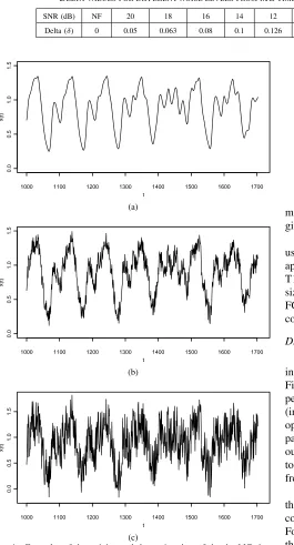
tox(1708)were used as basis for testing the systems. In this work, different versions of the training and the testing data are generated, i.e. the data is corrupted with a zero-mean uniform noise for different SNRs. We use 12 noise levels in training and testing data. Specifically, we use discretized levels from 0dB to 20dB with increments of 2, as well as the original NF data set (noise-free). Fig. 4 shows examples of the training and the testing data of the the MG time series at NF data and two different SNR level (10 and 0 dBs). Table I shows the delta (δ) values for different noise levels from MG time series training data corrupted by different levels of noise. These values are used to design the T1 non-singleton inputs and will be detailed in the next subsection.

C. Type-1 and Interval Type-2 Non-singleton Fuzzy Sets Cre-ation

In this step, first, the T1 non-singleton FS is initially de-signed by incorporating the information from the noise levels in each training data sets at different SNR level. From Table I, we can see that in NF data, the (δ) value is 0 by assuming that there is a relatively very small or no uncertainty/noise is present in the NF data. In this case the input is crisp value and modelled as a singleton FS as shown in Table II. Whereas, in the case shown in Table III, where value of delta (δ)= 0.159 at SNR = 10 dB, the input value is modelled as T1 non-singleton FS (see column 4). Note that the FOU size c in this case is equal to zero.

TABLE I

DELTA VALUES FOR DIFFERENT NOISE LEVELS FROMMGTIME SERIES CORRUPTED BY DIFFERENT LEVELS OF NOISE

SNR (dB) NF 20 18 16 14 12 10 8 6 4 2 0

Delta (δ) 0 0.05 0.063 0.08 0.1 0.126 0.159 0.20 0.252 0.317 0.399 0.502

1000 1100 1200 1300 1400 1500 1600 1700

0.0

0.5

1.0

1.5

t

x(t)

(a)

1000 1100 1200 1300 1400 1500 1600 1700

0.0

0.5

1.0

1.5

t

x(t)

(b)

1000 1100 1200 1300 1400 1500 1600 1700

0.0

0.5

1.0

1.5

t

x(t)

(c)

Fig. 4. Examples of the training and the testing data of the the MG time series. (a) NF data, where training is performed with 500 input-output pairs inx(1001), x(1002), . . . , x(1504)and testing is done with 200 input-output pairs inx(1505), x(1506), . . . , x(1708). (b) Training and testing data are corrupted with noise at SNR level 10dB and (c) at SNR level 0dB.

presented in Section II-B. First, the FOU size parameter

c ∈ [0,1] is discretized to a set of 11 values starting at 0 (T1 FS) and increasing to a maximum of 1.0 in increments of 0.1. For the FOU size parameter c = 0.0, the IT2 FSs reduce to the original T1 FSs, whereas for c = 1.0, the IT2 FS reachs the maximum amount of their width (i.e. the FOU covers the entire primary membership). Thus, we design 11 IT2 FSs, where each T1 FLS was designed using specific

TABLE II

ILLUSTRATION OF INPUT AT GIVENx0_WITHNFDATA

input δ singleton FS

NF x0 ₀

0

.0

1

.0

x'

modelled input FS with non-singleton T1/IT2 FSs with the given FOU size parameterc.

To construct the UMF and LMF of the input IT2 FSs, we use the FOU creation method detailed in Section II-B and apply equations (1) and (2) respectively by combining the T1 FSs with the chosen FOU size represented by the FOU size parameter c. An example of input FSs design using the FOU creation method at given x0 with MG time series data corrupted with 10db SNR level are shown in Table III.

D. Non-singleton Type-1 FLS Design and Rule Base Creation

In this step, the number of triangular MFs assigned to each input and output of the T1 FLS was chosen to be seven (see Fig. 3). While a higher number of MFs would enable a better performance, seven proved a good compromise for readability (in figures) and reasonable performance – in particular as optimal prediction performance is not a primary aim in this paper. First, we defined the FSs to evenly cover the input and output spaces. Then, we apply the WM method [32] in order to generate the rules from the given input-output pairs (noise-free training data).

The actual number of FSs and the rules are maintained from the T1 system designed based on the NF training data. All the common parameters of the SFLSs and NSFLSs are the same. For all experiments, σx in the NSFLS case is set equal to

the standard deviation of the additive noise. In a noise free situation for whichσx= 0, the performance of the NSFLS is

identical to that of the SFLS.

In the current paper, it is the input FSs only that are later modified to generate different T1 FLSs. The same rule base is employed for all FLSs in order to enable the comparison of all FLSs with a sole focus on their input FSs (rather than having differences differences in the rules). The resulting rules are used for all FLSs used in our experiments in order to enable a comparison which focuses on the inputs FSs.

E. T1/IT2 Non-Singleton T1 Fuzzy Logic Systems Evaluation

TABLE III

AN EXAMPLE OF INPUTFSDESIGN AT GIVENx0WITHMGTIME SERIES DATA CORRUPTED WITH10DBSNRLEVEL

input IT2 FSs at different FOU sizec

SNR

(dB) input δ c= 0 c= 0.5 c= 1.0

10 x0 0.159

0

.0

1

.0

δ

δ x' 0

.0

1

.0

c =0.5 _{T1 FS}

δ δ x'

UMF

LMF

0

.0

1

.0

T1 FS

δ δ x' c =1.0

UMF

LMF

sets are used to test the performance of the individual non-singleton T1 FLSs when faced the different uncertainty/noise levels. Now that we have 11 T1 FLSs, each using different FOU sizes determined by the given c, we test each of the FLSs against 12 levels of noise in order to determine which input FOU size results in the best performance for each given noise level. Each test is repeated 30 times to account for the random generation of the noise.

The performances of all the designs are evaluated using their root mean square error (RMSE) [14] based on (11), i.e.,

RM SE= v u u t

1 200

1707

X

k=1508

s(k+ 1)−f s(k)2

(11)

where, s(k + 1) is the output of the noisy testing data and f(s(k)_{) is the crisp output of the FLS, and, s}(k) ₌

[s(k−3), s(k−2), s(k−1), s(k)]T.

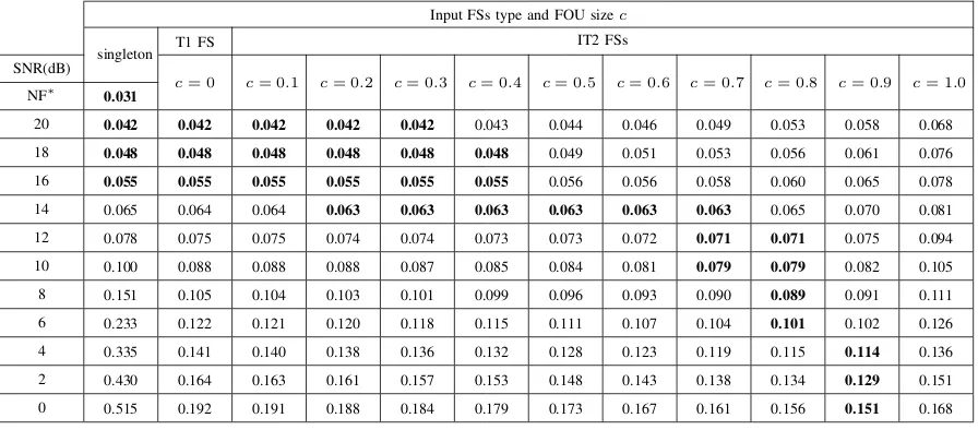
The RMSE results are averaged over 30 runs and are depicted in Table IV showing the results of the MG time series. Each column (except the 1st one that is showing singleton results) represents FLS design with a given FOU size parameter c whereas the rows show the average RMSE values for uniform noise at the different SNR values for all FOU sizes/FLSs. The bold values are the minimum of each average RMSE representing the best T1 FLS (based on the respective FOU size) at a particular SNR level.

IV. ANALYSIS ANDDISCUSSION

In this section, the experiment results are analysed and discussed. The presented experiments investigate modelling uncertainty in the input FSs using non-singleton fuzzification applied to the MG time series prediction.

The average RMSE values for the MG TSP using singleton and T1/IT2 (with different FOU sizes) non-singleton T1 FLS at different noise levels are depicted in Table IV. For a better illustration of the results in Table IV, we show a visual repre-sentation of the results in Fig. 5. This figure shows the RMSE values of SFLSs and NSFLSs using different noise levels (different SNR values) of testing data corrupted with different levels of noise for the MG time series. Fig. 5 illustrates the RMSE value of one singleton and 11 T1/IT2 non-singleton T1 FLSs using different noise levels at different SNR values

starting from noise free data (NF) and ending with the highest noise level (0dB) of the MG time series testing data. The eleven chosen FOU sizes in these experiments appear in the graph xaxis and each is tested at different noise level from NF to 0 dB. From Fig. 5, it is clear that there is a direct relationship between the input FOU size and the noise level in relation to the achieved performance. As the uncertainty/noise level increases (SNR decreases), the FOU size of the input FSs with best performance (i.e. giving the minimum RMSE value) increases.

The first column of Table IV contains the performance results of the singleton T1 FLS. The second column contains the results of T1 non-singleton T1 FLSs (designed using FOU size parameterc= 0.0 which reduces to the original T1 FS) tested at different noise levels. From these results, we can see that T1 non-singleton is outperforming singleton T1 FLS at all noise levels.

Moving to the right in Table IV, the FOU size parameterc

is increasing and the inputs modelling are transitioning from T1 (c = 0) to IT2 FSs that designed using the proposed FOU creation method with constant FOU size over the core of the primary membership domain. The performance clearly increases with the increased FOU size at each noise level. The reduction of the performance is started atc= 1.0 where the FOU covers the entire primary membership (i.e., LMF is entirely on the primary variable x–axis) [33], and only the UMF of the IT2 input FS is used in the fuzzification and accordingly is considered as T1 non-singleton fuzzification case (see the last column of Table III).

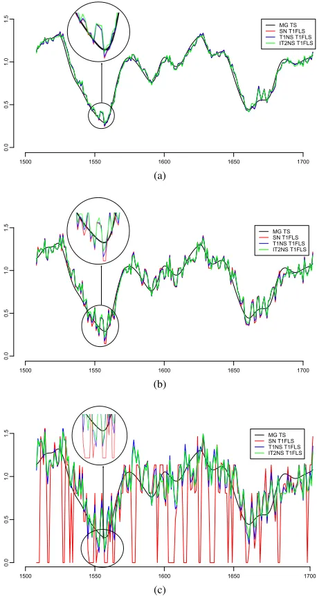
Finally, Fig. 6 shows a sample output of MG TSP using singleton T1 FLS and T1 non-singleton / IT2 non-singleton T1 FLSs with two different FOU sizes tested at three different chosen SNR levels: 20, 10 and 0 dBs. From the figure, we can note that the non-singleton T1 FLSs are performing better than singleton FLS especially at the higher level of uncertainty/noise such as 0dB. As the the FOU size of the IT2 FS increase the performance of IT2 non-singleton increases as well.

V. CONCLUSION

TABLE IV

THE AVERAGERMSEVALUES FOR THEMG TSPUSING SINGLETON ANDT1/IT2 (WITH DIFFERENTFOUSIZES)NON-SINGLETONT1 FLSS AT

DIFFERENT NOISE LEVELS. THE VALUES IN BOLD INDICATE THE MINIMUM OF EACH AVERAGERMSEREPRESENTING THE BESTFLS (BASED ON THE

RESPECTIVEFOUSIZE)AT A PARTICULARSNRLEVEL

Input FSs type and FOU sizec

T1 FS IT2 FSs

SNR(dB) singleton

NF∗ 0.031

c= 0 c= 0.1 c= 0.2 c= 0.3 c= 0.4 c= 0.5 c= 0.6 c= 0.7 c= 0.8 c= 0.9 c= 1.0

20 0.042 0.042 0.042 0.042 0.042 0.043 0.044 0.046 0.049 0.053 0.058 0.068

18 0.048 0.048 0.048 0.048 0.048 0.048 0.049 0.051 0.053 0.056 0.061 0.076

16 0.055 0.055 0.055 0.055 0.055 0.055 0.056 0.056 0.058 0.060 0.065 0.078

14 0.065 0.064 0.064 0.063 0.063 0.063 0.063 0.063 0.063 0.065 0.070 0.081

12 0.078 0.075 0.075 0.074 0.074 0.073 0.073 0.072 0.071 0.071 0.075 0.094

10 0.100 0.088 0.088 0.088 0.087 0.085 0.084 0.081 0.079 0.079 0.082 0.105

8 0.151 0.105 0.104 0.103 0.101 0.099 0.096 0.093 0.090 0.089 0.091 0.111

6 0.233 0.122 0.121 0.120 0.118 0.115 0.111 0.107 0.104 0.101 0.102 0.126

4 0.335 0.141 0.140 0.138 0.136 0.132 0.128 0.123 0.119 0.115 0.114 0.136

2 0.430 0.164 0.163 0.161 0.157 0.153 0.148 0.143 0.138 0.134 0.129 0.151

0 0.515 0.192 0.191 0.188 0.184 0.179 0.173 0.167 0.161 0.156 0.151 0.168

*NF: Noise Free Data

of a non-singleton FLS. The goal of this work is not to achieve the best performance in applications such as in time series prediction, but to study and present approaches for the modelling of uncertainty in FLS inputs using solely interval type-2 non-singleton fuzzification. The latter is valuable as the uncertainty in system inputs can directly be related to the FOU of the input FSs, while the rest of the FLS (antecedent and consequent FSs) can remain T1 FSs unless information on their respective uncertainty characteristics are known. This ap-proach is adopting an FOU creation method initially designed to determine an appropriate antecedent FS FOU and adjusted in this paper to generate appropriate FOUs for the input FSs based on input uncertainty, achieving potentially more efficient FLS design.

The proposed approach enables both the adaptation of the non-singleton IT2 FS for known levels of uncertainty (i.e. by increasing FOU size with increasing uncertainty) and the systematic comparison of the original T1 non-singleton T1 FLS to the resulting new IT2 non-singleton T1 FLS(s). This method shows the transitioning between different non-singleton FSs employed in different T1 FLSs showing best performance as the FOU size of employed IT2 FSs increases in relation to the increase of uncertainty/noise levels.

In order to explore the behaviour of the proposed approach, we conducted detailed performance comparison and evaluation in the context of time series analysis. The results indicate in general that T1 FLSs based on IT2 non-singleton FSs outperform those based on non-singleton T1 FS and singleton fuzzification. However, as the FOU size of the employed IT2 FS reached c = 1.0 the fuzzification process is converted into T1 non-singleton case because the FOU covers the entire primary membership. Only the UMF of the IT2 input FS is used in the fuzzification and accordingly is considered as T1

0 0.05 0.1 0.15 0.2 0.25 0.3 0.35 0.4 0.45 0.5 0.55 0.6

singleton 0 0.1 0.2 0.3 0.4 0.5 0.6 0.7 0.8 0.9 1

RM

SE

InputNFSN FOUNsize

NF 20 18 16 14 12 10 8 6 4 2 0

NoiseN Level

Fig. 5. RMSE value of one singleton and 11 T1/IT2 non-singleton T1 FLSs using different noise levels at different SNR values of the MG time series testing data

non-singleton fuzzification case resulting to reduction in the T1 FLS performance.

As part of future work, we will explore the methodological generation of both input FSs and the antecedents FSs of the system as an IT2 FSs to model both types of the uncertainties: uncertainty of the input data and the uncertainty associated with the linguistic terms of the FLS.

REFERENCES

[1] A. Saffiotti, “The uses of fuzzy logic in autonomous robot navigation,” Soft Computing, vol. 1, no. 4, pp. 180–197, 1997.

[2] H. Hagras, “Type-2 FLCs: A new generation of fuzzy controllers,”IEEE Comput. Intell. Mag., vol. 2, no. 1, pp. 30–43, Feb 2007.

[3] R. John and S. Coupland, “Type-2 fuzzy logic: A historical view,”IEEE Comput. Intell. Mag., vol. 2, no. 1, pp. 57–62, 2007.

[4] C. Wagner and H. Hagras, “Toward general type-2 fuzzy logic systems based on zSlices,”IEEE Trans. Fuzzy Syst., vol. 18, no. 4, pp. 637–660, 2010.

1500 1550 1600 1650 1700

0.0

0.5

1.0

1.5 _{MG TS}

SN T1FLS T1NS T1FLS IT2NS T1FLS

(a)

1500 1550 1600 1650 1700

0.0

0.5

1.0

1.5 MG TS

SN T1FLS T1NS T1FLS IT2NS T1FLS

(b)

1500 1550 1600 1650 1700

0.0

0.5

1.0

1.5 MG TS

SN T1FLS T1NS T1FLS IT2NS T1FLS

(c)

Fig. 6. Sample output of MG TSP using T1 FLS, T1NS T1 FLS (withc= 0) and IT2NS T1 FLS (withc= 0.5) at different SNR: (a) 20 dB , (b) 10 dB and (c) 0 dB.

systems using soft computing techniques (Advances in Soft Computing 41). Springer, 2007, pp. 16–25.

[6] H. Hagras, “A hierarchical type-2 fuzzy logic control architecture for autonomous mobile robots,”IEEE Trans. Fuzzy Syst., vol. 12, no. 4, pp. 524–539, 2004.

[7] G. Mouzouris and J. Mendel, “Non-singleton fuzzy logic systems,” in Proceedings of the Third IEEE Conference on Fuzzy Systems, IEEE World Congress on Computational Intelligence, vol. 1, 1994, pp. 456– 461.

[8] G. C. Mouzouris and J. M. Mendel, “Nonsingleton fuzzy logic systems: theory and application,”IEEE Trans. Fuzzy Syst., vol. 5, no. 1, pp. 56– 71, 1997.

[9] Q. Liang and J. Mendel, “Interval type-2 fuzzy logic systems: theory and design,”IEEE Trans. Fuzzy Syst., vol. 8, no. 5, pp. 535–550, 2000. [10] G. Mouzouris and J. Mendel, “Nonlinear time-series analysis with non-singleton fuzzy logic systems,” inProceedings of the IEEE/IAFE 1995 Computational Intelligence for Financial Engineering, 1995, pp. 47–56. [11] G. Mouzouris and J. Mendel, “Nonlinear predictive modeling using dynamic non-singleton fuzzy logic systems,” inProceedings of the Fifth IEEE International Conference on Fuzzy Systems, vol. 2, 1996, pp.

1217–1223.

[12] G. Mouzouris and J. Mendel, “Dynamic non-singleton fuzzy logic systems for nonlinear modeling,”IEEE Trans. Fuzzy Syst., vol. 5, no. 2, pp. 199–208, 1997.

[13] A. Perez-Neira, J. Sueiro, J. Roca, and M. Lagunas, “A dynamic non-singleton fuzzy logic system for DS/CDMA communications,” inIEEE International Conference on Fuzzy Systems Proceedings, IEEE World Congress on Computational Intelligence, vol. 2, 1998, pp. 1494–1499. [14] J. Mendel,Uncertain rule-based fuzzy logic systems: introduction and new directions. Upper Saddle River, NJ, USA: Prentice-Hall, 2001. [15] N. Sahab and H. Hagras, “A hybrid approach to modeling input variables

in non-singleton type-2 fuzzy logic systems,” in UK Workshop on Computational Intelligence (UKCI), 2010, pp. 1–6.

[16] D. Zhai, M. Hao, and J. Mendel, “A non-singleton interval type-2 fuzzy logic system for universal image noise removal using quantum-behaved particle swarm optimization,” inIEEE International Conference on Fuzzy Systems (FUZZ), 2011, pp. 957–964.

[17] N. Sahab and H. Hagras, “An adaptive type-2 input based nonsingleton type-2 fuzzy logic system for real world applications,” inIEEE Inter-national Conference on Fuzzy Systems (FUZZ), 2011, pp. 509–516. [18] N. Sahab and H. Hagras, “A type-2 nonsingleton type-2 fuzzy logic

system to handle linguistic and numerical uncertainties in real world environments,” inIEEE Symposium on Advances in Type-2 Fuzzy Logic Systems (T2FUZZ), 2011, pp. 110–117.

[19] A. Cara, I. Rojas, H. Pomares, C. Wagner, and H. Hagras, “On comparing non-singleton type-1 and singleton type-2 fuzzy controllers for a nonlinear servo system,” inIEEE Symposium on Advances in Type-2 Fuzzy Logic Systems (TType-2FUZZ), 2011, pp. 126–133.

[20] N. Sahab and H. Hagras, “Adaptive non-singleton type-2 fuzzy logic systems: a way forward for handling numerical uncertainties in real world applications,”Int. J. Comput. Commun. Control, vol. 5, no. 3, pp. 503–529, 2011.

[21] N. Sahab and H. Hagras, “Towards comparing adaptive type-2 input based non-singleton type-2 FLS and non-singleton FLSs employing gaussian inputs,” in IEEE International Conference on Fuzzy Systems (FUZZ-IEEE), 2012, pp. 1–8.

[22] A. Cara, C. Wagner, H. Hagras, H. Pomares, and I. Rojas, “Multiobjec-tive optimization and comparison of nonsingleton type-1 and singleton interval type-2 fuzzy logic systems,”IEEE Trans. Fuzzy Syst., vol. 21, no. 3, pp. 459–476, 2013.

[23] A. Pourabdollah, C. Wagner, M. Smith, and K. Wallace, “Real-world utility of non-singleton fuzzy logic systems: A case of environmental management,” in IEEE International Conference on Fuzzy Systems (FUZZ-IEEE), 2015, pp. 1–8.

[24] A. Pourabdollah, C. Wagner, and J. Aladi, “Changes under the hood-a new type of non-singleton fuzzy logic system,” in IEEE International Conference on Fuzzy Systems (FUZZ-IEEE), 2015, pp. 1–8.

[25] J. Aladi, C. Wagner, and J. Garibaldi, “Type-1 or interval type-2 fuzzy logic systems -on the relationship of the amount of uncertainty and FOU size,” inIEEE International Conference on Fuzzy Systems (FUZZ-IEEE), 2014, pp. 2360–2367.

[26] J. H. Aladi, C. Wagner, J. M. Garibaldi, and A. Pourabdollah, “On transitioning from type-1 to interval type-2 fuzzy logic systems,” in IEEE International Conference on Fuzzy Systems (FUZZ-IEEE), 2015, pp. 1–8.

[27] J. Jang and C. Sun, “Predicting chaotic time series with fuzzy if–then rules,” inSecond IEEE Int. Conf. on Fuzzy Systems, 1993, pp. 1079– 1084.

[28] N. N. Karnik and J. M. Mendel, “Applications of type-2 fuzzy logic systems to forecasting of time-series,”Information Sciences, vol. 120, no. 1, pp. 89–111, 1999.

[29] M. Versaci and F. C. Morabito, “Fuzzy time series approach for disruption prediction in Tokamak reactors,”IEEE Trans. Magn., vol. 39, no. 3, pp. 1503–1506, 2003.

[30] M. C. Mackey and L. Glass, “Oscillation and chaos in physiological control systems,”Science, vol. 197, no. 4300, pp. 287–289, 1977. [31] D. A. Quinney,An Introduction to the Numerical Solution of Differential

Equations. New York, NY, USA: John Wiley & Sons, Inc., 1987. [32] L. Wang and J. M. Mendel, “Generating fuzzy rules by learning from

examples,” IEEE Trans. Syst., Man, Cybern., vol. 22, no. 6, pp. 1414 –1427, 1992.