Leaf segmentation in plant phenotyping: a collation study

Hanno Scharr · Massimo Minervini · Andrew P. French · Christian Klukas · David M. Kramer · Xiaoming Liu · Imanol Luengo Munti´on · Jean-Michel Pape · Gerrit Polder · Danijela Vukadinovic · Xi Yin · Sotirios A. Tsaftaris

Leaf segmentation in plant phenotyping: A collation study

Received: date / Accepted: date

MM and SAT acknowledge a Marie Curie Action: “Reintegra-tion Grant” (grant #256534) of the EU’s Seventh Framework Programme (FP7/2007-2013). HS acknowledges funding from EU-FP7 no. 247947 (GARNICS). HS, JMP and CK acknowl-edge the support of the German-Plant-Phenotyping Network, which is funded by the German Federal Ministry of Educa-tion and Research (project identificaEduca-tion number: 031A053). XY, XL, and DK acknowledge the support of US Department of Energy, Office of Science, Basic Energy Sciences Program (DE-FG02-91ER20021) and the MSU Center for Advanced Algal and Plant Phenotyping.

Author contributions: SAT coordinated this collation study. SAT and HS organized the original LSC challenge. SAT, HS, and MM, wrote the paper and performed analy-sis. All other authors have contributed methods, text, and results. All authors have approved the manuscript.

H. Scharr

Institute of Bio- and Geosciences: Plant Sciences (IBG-2) Forschungszentrum J¨ulich GmbH, J¨ulich, Germany

E-mail: [email protected]

M. Minervini

IMT Institute for Advanced Studies, Lucca, Italy E-mail: [email protected]

A.P. French·I. Munti´on

Schools of Biosciences and Computer Science, Centre for Plant Integrative Biology, University of Nottingham, UK E-mail:{Andrew.P.French, psxil1}@nottingham.ac.uk

C. Klukas·J.-M. Pape

Dept. of Molecular Genetics, Leibniz Institute of Plant Genet-ics and Crop Plant Research (IPK), Gatersleben, Germany E-mail:{pape, klukas}@ipk-gatersleben.de

D.M. Kramer

Depts. of Energy Plant Research Lab, and Biochemistry and Molecular Biology, Michigan State University

E-mail: [email protected]

X. Liu·X. Yin

Dept. of Computer Science and Engineering, Michigan State University

E-mail:{liux, yinxi1}@cse.msu.edu

G. Polder·D. Vukadinovic

Greenhouse Technology Group, Wageningen University and Research Centre, Wageningen, Netherlands

E-mail:{gerrit.polder, danijela.vukadinovic}@wur.nl

Abstract Image-based plant phenotyping is a growing application domain of computer vision in agriculture. A key task is the segmentation of all individual leaves in im-ages. Here we focus on the most common rosette model plants Arabidopsis and young tobacco. Although leaves do share appearance and shape characteristics, the pres-ence of occlusions and variability in leaf shape and pose, as well as imaging conditions, render this problem chal-lenging. The aim of this paper is to compare several leaf segmentation solutions on a unique and first of its kind dataset containing imagesfrom typical phenotyping ex-periments. In particular, we report and discuss meth-ods and findings of a collection of submissions for the first Leaf Segmentation Challenge (LSC) of the Com-puter Vision Problems in Plant Phenotyping (CVPPP) workshop in 2014. Four methods are presented: three segment leaves via processing the distance transform in an unsupervised fashion, and the other via optimal tem-plate selection and Chamfer matching. Overall, we find that although separating plant from background can be achieved with satisfactory accuracy (>90% Dice score), individual leaf segmentation and counting remain chal-lenging when leaves overlap. Besides, accuracy is lower for younger leaves. We find also that variability in datasets does affect outcomes. Our findings motivate further in-vestigations and development of specialized algorithms for this particular application, and that challenges of this form are ideally suited for advancing the state of the art. Data are publicly available (

http://www.plant-phenotyping.org/CVPPP2014-dataset) to support

fu-ture challenges beyond segmentation within this appli-cation domain.

Keywords plant phenotyping · leaf · multi-instance segmentation·machine learning

S.A. Tsaftaris ( )

IMT Institute for Advanced Studies, Lucca, Italy, and Institute for Digital Communications, School of Engineering, University of Edinburgh, Edinburgh, UK

1 Introduction

The study of a plant’s phenotype, i.e., its performance and appearance, in relation to different environmental conditions is central to understanding plant function. Identifying and evaluating phenotypes of different cul-tivars (or mutants) of the same plant species, are rele-vant to, e.g., seed production and plant breeders. One of the most sought-after traits is plant growth, i.e., a change in mass, which directly relates to yield. Biolo-gists grow model plants, such as Arabidopsis ( Arabidop-sis thaliana) and tobacco (Nicotiana tabacum), in con-trolled environments and monitor and record their phe-notype to investigate general plant performance. While previously such phenotypes were annotated manually by experts, recently image-based nondestructive approaches are gaining attention among plant researchers to measure and study visual phenotypes of plants [24, 28, 41, 55].

In fact, most experts now agree that lack of reliable and automated algorithms to extract fine-grained infor-mation from these vast datasets forms a new bottleneck in our understanding of plant biology and function [39]. We must accelerate the development and deployment of such computer vision algorithms, since according to the Food and Agriculture Organization of the United Na-tions (FAO), large-scale experiments in plant phenotyp-ing are a key factor in meetphenotyp-ing agricultural needs of the future, one of which is increasing crop yield for feeding 11 billion people by 2050.

Yield is related to plant mass and the current gold standard for measuring mass is weighing the plant, how-ever this is invasive and destructive. Show-everal specialized algorithms have been developed to measure whole-plant properties and particularly plant size [6, 17, 25, 27, 31, 40, 55, 61]. Nondestructive measurement of a plant’s pro-jected leaf area (PLA), i.e., the counting of plant pix-els from top-view images, is considered a good approx-imation of plant size for rosette plants and is currently used. However, when considering growth, PLA reacts rel-atively weakly, as it includes growing and non-growing leaves, but the per leaf derived growth (implying a per leaf segmentation), has a faster and clearer response. Thus, for example, growth regulation [5] and stress situ-ations [28] can be evaluated in more detail. Additionally, since growth stages of a plant are usually based on the number of leaves [15], an estimate of leaf count as pro-vided by leaf segmentation is beneficial.

However, obtaining such refined information at the individual leaf level (as for example in [56]), which could help us identify even more important plant traits, from a computer vision perspective is particularly challeng-ing. Plants are not static, but self-changing organisms with complexity in shape and appearance increasing over time. In the range of hours leaves move and grow, with the whole plant changing over days or even months, in which the surrounding environmental (as well as mea-surement) conditions may also vary.

Fig. 1: Example images of Arabidopsis and tobacco from the datasets used in this study [48].

Considering also the presence of occlusions, it is not surprising that the segmentation of leaves from single view images (a multi-instance image segmentation prob-lem), remains an unsolved problem even in the controlled imaging of model plants. Motivated by this we organized the Leaf Segmentation Challenge (LSC) of the Computer Vision Problems in Plant Phenotyping (CVPPP 2014) workshop,1 _{held in conjunction with the 13}th _European Conference on Computer Vision (ECCV), to assess the current state of the art.

This paper offers a collation study and analysis of several methods from the LSC challenge but also from the literature. We briefly describe the annotated dataset, the first of its kind, that was used to test and evaluate the methodsfor the segmentation of individual leaves in image-based plant phenotyping experiments (see Figure 1 and also [48]). Color images in the dataset show top-down views on rosette plants. Two datasets show differ-ent cultivars of Arabidopsis (A. thaliana) while another one shows tobacco (N. tabacum) under different treat-ments. We manually annotated leaves in these images to provide ground-truth segmentation and defined ap-propriate evaluation criteria. Several methods are briefly presented in a dedicated section and in the results section we discuss and evaluate each method.

The remainder of this article is organized as follows: Section 2 offers a short literature review, while Section 3 defines the adopted evaluation criteria. Section 4 presents

1

the datasets and annotations used to support the LSC challenge, which is described in Section 5. Section 6 de-scribes the methods compared in this study, with their performance and results discussedin Section 7. Finally, Section 8 offers conclusionsand outlook.

2 Related work

At first glance the problem of leaf segmentation appears similar to leaf identification and isolated leaf segmenta-tion(see e.g. [12–14, 30, 50, 59]), although as we will see later it is not. Research on these areas has been moti-vated by several datasets showing leaves in isolation cut from plants and imaged individually, or showing leaves on the plant but with a leaf encompassing a large field of view (e.g., by imaging via a smart phone application). This problem has been addressed in an unsupervised[50, 59], shape-based[13, 14, 30], and interactive[12–14] fash-ion.

However, the problem at hand is radically different. The goal, as the illustrative example of Figure 1 shows, is not to identify the plant species (usually known in this context) but to segment accurately each leaf in an image showing a plant. This multi-instance segmenta-tion problem is excepsegmenta-tionally complex in the context of this application. This is due to the variability in shape, pose, and appearance of leaves, but also due to lack of clearly discernible boundaries among overlapping leaves with typical imaging conditions where a top-view fixed camera is used. Several authors have dealt with the seg-mentation of a live plant from background to measure growth using unsupervised [17, 25] and semi-supervised methods [36], but not of individual leaves. The use of color in combination with depth images or multiple im-ages for supervised or unsupervised plant segmentation is also common practice [4, 10, 29, 46, 49, 51, 52, 57].

Several authors have considered leaf segmentation in a tracking context, where temporal information is avail-able. For example, Yin et al. [61] segment and track the leaves of Arabidopsis in fluorescence images using a Chamfer-derived energy functional to match available segmented leaf templates to unseen data. Dellen et al. [18] use temporal information in a graph based formulation to segment and track leaves in a high spatial and tempo-ral resolution sequence of tobacco plants. Aksoy et al. [3] track leaves over time, merging segments derived by su-perparametric clustering by exploiting angular stability of leaves. De Vylder et al. [16] use an active contour formulation to segment and track Arabidopsis leaves in time-lapse fluorescence images.

Even in the general computer vision literature, this type of similar appearance, multi-instance problem is not well explored. Although several interactive approaches exist [23, 42], user interaction inherently limits through-put. Therefore, here we discuss automated learning-based object segmentation approaches, which might be

adapt-able to leaf segmentation. Wu and Nevatia [58] present an approach that detects and segments multiple, par-tially occluded objects in images, relying on a learned, boosted whole-object segmentor and several part detec-tors. Given a new image, pixels showing part responses are extracted and a joint likelihood estimation inclu-sive of inter-object occlusion reasoning is maximized to obtain final segmentations. Notably, they test their ap-proach on classical pedestrians datasets, where appear-ance and size variation does exist, so in leaf segmenta-tion where neighboring leaves are somewhat similar this approach might yield less appealing results. Another in-teresting work [47] relies on Hough voting to jointly de-tect and segment objects. Interestingly, beyond pedes-trian datasets they also use a dataset of house windows where appearance and scale variation is high (as is com-mon also in leaves), but they do not overlap. Finally, graphical methods have also been applied to resolve and segment overlapping objects [26], and were tested also on datasets showing multiple horses.

Evidently, till now the evaluation and development of leaf segmentation algorithms using a common reference dataset of individual images without temporal informa-tion is lacking, and is the main focus of this paper.

3 Evaluation measures

Measuring multi-object segmentation accuracy is an ac-tive topic of research with several metrics previously pro-posed [33–35, 44]. For the challenge and this study, we adopted several evaluation criteria and devised Matlab implementations. Some of these metrics are based on the Dice score of binary segmentations:

Dice (%) = 2|P

gt_∩Par_|

|Pgt_|+|Par_|, (1)

measuring the degree of overlap among ground truthPgt

and algorithmic resultPar _{binary segmentation masks.}

Overall, two groups of criteria were used. To evaluate segmentation accuracy we used:

– Symmetric Best Dice (SBD), the symmetric

aver-age Dice among all objects (leaves), where for each input label the ground truth label yielding maximum Dice is used for averaging, to estimate average leaf segmentation accuracy. Best Dice (BD) is defined as:

BD(La, Lb) = 1 M

M X

i=1 max 1≤j≤N

2|La i ∩Lbj|

|La i|+|Lbj|

, (2)

and Lb, respectively. SBD between Lgt, the ground truth, andLar, the algorithmic result, is defined as:

SBD(Lar, Lgt) = min

BD(Lar, Lgt),BD(Lgt, Lar) . (3)

– Foreground-Background Dice (FBD), the Dice score

of the foreground mask (i.e., the whole plant assum-ing the union of all leaf labels), to evaluate a de-lineation of a plant from the background obtained algorithmically with respect to the ground truth.

We should note that we also considered the Global Con-sistency Error (GCE) [34] and Object-level ConCon-sistency Error (OCE) [44] metrics, which are suited for evaluat-ing segmentation of multiple objects. However, we found that they are harder to interpret and that the SBD is capable of capturing relevant leaf segmentation errors.

To evaluate how good an algorithm is in identifying the correct number of leaves present, we relied on:

– Difference in Count (DiC), the number of leaves

in algorithm’s result minus the ground truth:

DiC = #Lar−#Lgt. (4)

– |DiC|, the absolute value ofDiC.

In addition to the metrics adopted for the challenge, in Section 7.5 we augment our evaluation with metrics that prioritize leaf shape and boundary accuracy.

4 Leaf data and manual annotations 4.1 Imaging setup and protocols

We devised imaging apparatuses, setups, and experiments emulating typical phenotyping experiments, to acquire three imaging datasets, summarized in Table 1, to sup-port this study. They were acquired in two different labs with highly diverse equipment. Detailed information is available in [48], but brief descriptions are given below for completeness.

Arabidopsis data: Arabidopsis images were acquired in two data collections, in June 2012 and in September-October 2013, hereafter named Ara2012 and Ara2013, respectively, both consisting of top-view time-lapse im-ages of severalArabidopsis thaliana rosettes arranged in trays. Arabidopsis images were acquired using two setups for investigating affordable hardware for plant phenotyp-ing.2 Images were captured during day time only, every 6 hours over a period of 3 weeks for Ara2012, and every 20 minutes over a period of 7 weeks for Ara2013. Two cameras were used: a 7 megapixel commercial grade cam-era (Canon PowerShot SD1000), shorthanded asCanon, and an even lower cost system based on the Rasberry

2

http://www.phenotiki.com

Pi, Model B, with the Rasberry Pi 5 megapixel camera module. In this study only Canon data are used.

Acquired raw images (3108×2324 pixels, pixel size of ∼0.167 mm) were first developed into an uncompressed (TIFF) format, and subsequently encoded using the loss-less compression standard available in the PNG file for-mat [54].

Tobacco data: Tobacco images were acquired using a robotic imaging system for the investigation of auto-mated plant treatment optimization by an artificial cog-nitive system.3 _{The robot head consisted of two stereo} camera systems, black-and-white and color, each consist-ing of 2 Point-Grey Grashopper cameras with 5 megapixel (2448×2048, pixel size 3.45µm) resolution and high qual-ity lenses (Schneider Kreuznach Xenoplan 1.4/17-0903). We added lightweight white and NIR LED light sources to the camera head.

Using this setup, each plant was imaged separately from different but fixed poses. In addition, for each pose small baseline stereo image pairs were captured using each single camera, respectively, by a suitable robot move-ment, allowing for 3D reconstruction of the plant. For the top view pose, distance between camera center and top edge of pot varied between 15 cm and 20 cm for differ-ent plants, but being fixed per plant, resulting in lateral resolutions between 20 and 25 pixel/mm.

Data used for this study stemmed from experiments aiming at acquiring training data and contained a sin-gle plant imaged directly from above (top-view). Images were acquired every hour, 24/7, for up to 30 days.

4.2 Selection of data for training and testing

As part of the benchmark data for the LSC we released three datasets, named respectively ‘A1’, ‘A2’, and ‘A3’, consisting of single-subject images of Arabidopsis and tobacco plants, each accompanied by manual annotation (discussed in the next section) of plant and leaf pixels. Examples are shown in Figure 1.

From the Ara2012 dataset, to form the ‘A1’ dataset we extracted (by cropping) from tray images, 161 indi-vidual plant images (500×530 pixels), spanning a period of 12 days. Additional 40 images (530×565 pixels) form ‘A2’, which were extracted from the Ara2013 dataset spanning a period of 26 days. From the tobacco data-set, to form the ‘A3’ dataset we extracted 83 images (2448×2048 pixels). Each dataset was split into training and testing sets for the challenge (cmp. Section 5).

The data differ in resolution, fidelity, and scene com-plexity, with plants appearing in isolation or together with other plants (in trays), with plants belonging to different cultivars (or mutants), and subjected to differ-ent treatmdiffer-ents.

Due to the complexity of the scene and of the plant objects, the datasets present a variety of challenges with

3

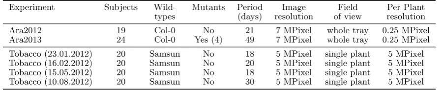
Table 1: Summary of information of the Arabidopsis and tobacco experiments providing the three datasets.

Experiment Subjects Wild- Mutants Period Image Field Per Plant types (days) resolution of view resolution

Ara2012 19 Col-0 No 21 7 MPixel whole tray 0.25 MPixel

Ara2013 24 Col-0 Yes (4) 49 7 MPixel whole tray 0.25 MPixel

Tobacco (23.01.2012) 20 Samsun No 18 5 MPixel single plant 5 MPixel Tobacco (16.02.2012) 20 Samsun No 20 5 MPixel single plant 5 MPixel Tobacco (15.05.2012) 20 Samsun No 18 5 MPixel single plant 5 MPixel Tobacco (10.08.2012) 20 Samsun No 30 5 MPixel single plant 5 MPixel

respect to analysis. Since our goal was to produce a good variety of images, images corresponding to several chal-lenging situations were included.

Specifically, in ‘A1’ and ‘A2’, occasionally, a layer of water in the tray due to irrigation causes reflections. As the plants grow, leaves tend to overlap, resulting in se-vere leaf occlusions. Nastic movements (a movement of a leaf usually on the vertical axis) make leaves appear of different shape and size from one time instant to an-other.In‘A3’ beneath shape changes due to nastic move-ments, also different leaf shapes appear due to differ-ent treatmdiffer-ents. Under high illumination conditions (one of the treatment options in the Tobacco experiments), plants stay more compact with partly wrinkled leaves, severely overlapping. Under lower light conditions, leaves are more round and larger.

Furthermore, ‘A1’ presents a complex and changing background, which could complicate plant segmentation. A portion of the scene is slightly out of focus (due to the large field of view) and appears blurred, and some images include external objects such as tape or other fiducial markers. In some images, certain pots have moss on the soil, or have dry soil and appear yellowish (due to increased ambient temperature for a few days). ‘A2’ presents a simpler scene (e.g., more uniform background, sharper focus, without moss); however, it includes mu-tants with different phenotypes related to rosette size (some genotypes produce very small plants) and leaf ap-pearance with major differences in both shape and size. ‘A3’ presents much higher image resolution, making computational complexity more relevant. Additionally, in ‘A3’ plants undergo a wide range of treatments chang-ing their appearance dramatically, while Arabidopsis is known to have different leaf shape among mutants. Fi-nally, self-occlusion, shadows, leaf hairs, leaf color varia-tions and others, make the scene even more complex.

4.3 Annotation strategy

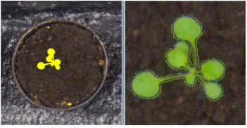
Figure 2 depicts the procedure we followed to anno-tate the image data. In the first place, we obtained a binary segmentation of the plant objects in the scene in a computer-aided fashion. For Arabidopsis, we used the approach based on active contours described in [36], while for tobacco, a simple color-based approach for plant

Original Image Plant Segmentation Leaf Segmentation

Fig. 2: Schematic of the workflow to annotate the images. Plants were first delineated in the original image, then individual leaves were labeled.

segmentation was used. The result of this segmentation was manually refined using raster graphics editing soft-ware. Next, within the binary mask of each plant, we delineated individual leaves, following an approach com-pletely based on manual annotation. A pixel with black color denotes background, while all other colors are used to uniquely identify the leaves of the plants in the scene. Across the frames of the time-lapse sequence, we consis-tently used the same color code to label the occurrences of the same leaf. The labeling procedure involved always two annotatorsto reduce observer variability, one anno-tating the dataset and one inspecting the other.

Note that LSC did not involve leaf tracking over time, therefore all individual plant images were considered sep-arately, ignoring any temporal correspondence.

4.4 File types and naming conventions

Plant images were encoded using the lossless PNG [54] format and their dimensions varied. Plant objects ap-peared centered in the (cropped) image. Segmentation masks were image files encoded as indexed PNG, where each segmented leaf is identified with a unique (per im-age) integer value, starting from ‘1’, whereas ‘0’ denotes background. The union of all pixel labels greater than zero provides the ground truth plant segmentation mask. A color index palette was included within the file for vi-sualization reasons. The filenames have the form:

– plantXXX_rgb.png: the original RGB color image;

– plantXXX_label.png: the labeled image;

5 CVPPP 2014 LSC challenge outline

The LSC challenge was organized by two of the authors (HS and SAT), as part of the CVPPP workshop, which was held in conjunction with the European Conference on Computer Vision (ECCV), in Z¨urich, Switzerland, in September 2014. Electronic invitations for participa-tion were communicated to a large number of researchers working on computer vision solutions for plant pheno-typing and via computer vision and pattern recognition mailing lists and several phenotyping consortia and net-works such as DPPN,4 _IPPN,5 _EPPN,6 _iPlant.7 Inter-ested parties were asked to visit the website and register for the challenge after agreeing to rules of participation and providing contact info via an online form.

Overall, 25 teams registered for the study and down-loaded training data, 7 downdown-loaded testing data, and fi-nally 4 submitted manuscript and testing results for re-view at the workshop. For this study we invited several of the participants (see Section 6).

5.1 Training phase

An example preview of the training set (i.e., one example image from each of the three datasets as shown in Fig-ure 1) was released in March 2014 on the CVPPP 2014 website. The full training set, consisting of color images of plants and annotations, was released in April 2014.

A total of 372 PNG images were available in 186 pairs of raw RGB color images and corresponding annotations in the form of indexed images, namely 128, 31, and 27 images for ‘A1’, ‘A2’, and ‘A3’, respectively. Images of many different plants were included at different time points (growth stages). Participants were unaware of any temporal relationships among images, and were expected to treat each image in an individual fashion. Partici-pants were allowed to tailor pipelines to each dataset and could choose supervised or unsupervised methods. Matlab evaluation functions were also provided to help participants assess performance on the training set using the criteria discussed in Section 3. We should note that data and evaluation script are in the public domain.8

5.2 Testing phase

We released 98 color images for testing (i.e., 33, 9, and 56 for ‘A1’, ‘A2’, and ‘A3’, respectively) and kept the re-spective label images hidden. Images here corresponded to plants at different growing stage (with respect to those

4

http://www.dppn.de/ 5

http://www.plant-phenotyping.org/ 6

http://www.plant-phenotyping-network.eu/ 7

http://www.iplantcollaborative.org/ 8

http://www.plant-phenotyping.org/CVPPP2014-dataset

included in the training set) or completely new and un-seen plants. Again this was unknown to the participants. A short testing period was allowed: the testing set was released on June 9, 2014, and authors were asked to sub-mit their results by June 17, 2014, and accompanying papers by June 22, 2014.

In order to assess the performance of their algorithm on the test set, participants were asked to email to the organizers a ZIP archive following a predefined folder/file structure that enabled automated processing of the re-sults. Within 24 hours all participants who submitted testing results received their evaluation using the same evaluation criteria as for training, as well as summary tables in LA_{TEX and also individual per image results in} a CSV format. Algorithms and the papers were subject to peer review and the leading algorithm [43] presented at the CVPPP workshop.

6 Methods

We briefly present the leaf segmentation methods used in this collation study. We include methods not only from challenge participants but also others for completeness and for offering a larger view of the state of the art. Overall, three methods rely on post-processing of dis-tance maps segment leaves, while one uses a database of templates which are matched using a distance metric. Each method’s description aims to provide an under-standing of the algorithms, and wherever appropriate we offer relevant citations to background for readers seeking additional information.

Please note that participating methods were given access to the training set (including ground truth) and testing set but without ground truth.

6.1 IPK Gatersleben: Segmentation via 3D histograms

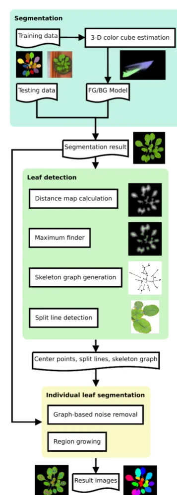
The IPK pipeline relies on unsupervised clustering and distance maps to segment leaves. Details can be found in [43]. The overall workflow is depicted in Figure 3 and summarized in the following.

1. Supervised foreground/background segmentation uti-lizing 3D histogram cubes, which encode the proba-bility for any observed pixel color in the given train-ing to belong to the fore- or background; and 2. Unsupervised feature extraction of leaf-center points

and leaf-split point detection for individual leaf seg-mentation by using a distance map, skeleton, and the corresponding graph representation (cmp. Figure 3).

Fig. 3: Workflow of the IPK approach, including main processing components: segmentation, image feature ex-traction (including leaf detection) and individual leaf segmentation.

are accumulated using the provided training data. To improve the performance against illumination variabil-ity, input images are converted into theLab color space [7].Entries which are not represented in the training data are estimated by using an interpolation of the surround-ing values of a histogram cell. The segmentation results are further processed by morphological operations and

cluster-analysis to suppress noise and artifacts. The out-come of this operation serves as input for the feature ex-traction phase to detect leaf center-points and optimal split-points of corresponding leaf segments.

For this approach, the leaves of Arabidopsis plants in ‘A1’ and ‘A2’ are considered as compact objects which only partly overlap. In the corresponding Euclidean dis-tance map (EDM) the leaf center points appear as peaks, which are detected by a maximum search. At a next step, a skeleton image is calculated. To resolve leaf-overlaps, split-points at the thinnest connection points are de-tected. Values of the EDM are mapped on the skeleton image. The resulting image is used for creating a skele-ton graph, where leaf center points, skeleskele-ton end-points, and skeleton branch-points are represented as nodes in the graph. Edges are created if the corresponding image points are connected by a skeleton line. Additionally, a list of the positions and minimal distances of each par-ticular edge segment are saved as an edge-attribute. This list is used to detect the exact positions of the leaf split points. To find the split point(s) between two leaf center points and therefore graph nodes, all edges of the graph structure connecting these two points are traversed and the position with the minimal EDM value is determined. This process is repeated, if there are still connections between the two leaves which need to be separated. For calculating the split line belonging to a particular mini-mal EDM point, two coordinates on the plant leaf border are calculated. The nearest background pixel is searched (first point), and also the nearest background pixel at the opposite position relative to the split point (second point) is located. The connection line is used as border during the segmentation of overlapping leaves. In a final step the separated leaves are labeled by a region-growing algorithm.

Our approach was implemented in Java, and tested on a desktop PC with 3.4 GHz processor and 32 GB mem-ory. Java was configured to use a maximum of 4 GB RAM (-Xmx4g). On average each image takes 1.6, 1.2, and 9 seconds for ‘A1’, ‘A2’, and ‘A3’, respectively.

6.2 Nottingham: Segmentation with SLIC superpixels

A superpixel-based method that does not require any training is used. The training dataset has been used for parameter tuning only. The processing steps visualized in Figure 5 can be summarized as follows:

1. Superpixel over-segmentation inLab color-space us-ing SLIC[1];

2. Foreground (plant) extraction using simple seeded re-gion growing in the superpixel space;

3. Distance map calculation on extracted foreground; 4. Individual leaf seed matching by identifying the

Fig. 4: Example images of each of the steps in the Not-tingham approach. First row: original image (left), SLIC superpixels (center), thresholded superpixels (right). Second row: distance map with superpixel centroids (left), filtered superpixel centroids (middle), watershed segmentation (right).

Fig. 5:The Nottingham leaf segmentation process.

5. Individual leaf segmentation by applying watershed transform with the extracted seeds.

Steps 1) and 2) are used to extract the whole plant while 3), 4) and 5) for extracting individual leafs. Fol-lowing is a detailed explanation of each of the steps with Figures 4 and 5 summarizing the process.

Preparation. Given an RGB image, it is first con-verted to theLab color space [7], to enhance discrimina-tion between foreground leaves and background. Then, SLIC superpixels [1] are computed. A fixed number of su-perpixels is computed over the image. Empirically, 2000 pixels was found to provide good coverage of the leaves. The mean color of the ‘a’ channel (which characterizes well the green color of the image) is extracted for each superpixel. A Region Adjacency Map (superpixel neigh-borhood graph) is created from the resulting superpixels.

Foreground extraction. Having the mean color of each superpixel for channel ‘a’, a simple region growing ap-proach [2] in superpixel space allows the complete plant to be extracted. The superpixel with the lowest mean

color (the most bright green superpixel) defined in Lab space is used as the initial seed. However, for ‘A1’ and ‘A2’, since they do not contain shadows, an even sim-pler thresholding of the mean color of each superpixel allows faster yet still accurate segmentation of the plant. Thresholds for the ‘A1’ and ‘A2’ are set to−25 and−15 respectively.

Leaf identification. Once the plant is extracted from the background, superpixels not belonging to the plant are removed. A distance map is computed (first remov-ing strong edges usremov-ing the Canny detector [11]) and the centroids are calculated for all superpixels. A local max-ima filter is applied to extract the superpixels that lay in the center of the leaves. A superpixel is selected as a seed only if its centroid is best-centered in the leaf compared to its neighbors within a radius. This is im-plemented by considering the superpixel centroid value in the already calculated distance map, and filtering the superpixels that do not have the maximum value within its neighbors.

Leaf segmentation. Finally, watershed segmentation [53] is applied with the obtained initial seeds over the image space, yielding the individual leaf segmentation.

Using a Python implementation running on a i3 quad-core desktop with i3-4130 (3.4 GHz) processor and 8 GB memory, on average each image takes < 1 second for dataset ‘A1’ and ‘A2’, and 1-5 seconds for ‘A3’.

Overall, it is a fast method with no training required. It also could be tuned to get a much higher accuracy on a per-image basis. The parameters that can be tuned are: (1) number of superpixels, (2) compactness of su-perpixels, (3) foreground extractor (threshold or region growing), (4) parameters of the canny edge detector, (5) color space for SLIC, foreground extractor and canny edge detector. All those parameters were tuned in a per dataset basis using the training set in order to maximize the mean Symmetric Best Dice score for each dataset. However, they can be easily tuned manually on a per image basis if required.

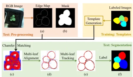
6.3 MSU: Leaf segmentation with Chamfer matching

The MSU approachextends a multi-leaf alignment and tracking framework[60–62]to the LSC. As discussed in Section 2 this framework was originally designed for seg-menting and tracking leaves in fluorescence plant videos where plant segmentation is straightforward due to the clean background. For LSC, amore advancedbackground segmentation process was adopted.

Chamfer Matching RGB Image

Template Generation

Labeled Images Edge Map Mask

Multi-leaf Alignment

Multi-leaf

Tracking Label

Test: Pre-processing

Test: Segmentation

Training: Templates (a) (b)

(c) (d) (e) (f)

Fig. 6: Overview of the MSU approach: training is done once for each plant type (i.e., twice for three datasets), and pre-processing and segmentation are performed for each image.

from H images of the training set. Each leaf shape is scaled toS different sizes, and each size is rotated to R different orientations. This leads to a set of H×S×R leaf templates (5×9×24 for ‘A1’ and ‘A2’, 8×10×24 for ‘A3’) with labeled tip locations, which will be used in the segmentation process.

An accurate plant segmentation and edge map are critical to obtain reliable CM results. To this end, all RGB images are converted into theLabcolor space, and a threshold τ is applied to channel ‘a’ for estimating a foreground mask (chosen empirically for each dataset: 40 for ‘A1’, and 30 for ‘A2’ and ‘A3’), which is refined by standard morphological operations. TheSobeledge oper-ator is applied within the foreground segment to generate an edge map. Since ‘A3’ has more overlapping leaves and the boundaries between the leaves are more visible due to shadows, an additional edge map is used, obtained by applying the edge operator on the image resulting as the difference of ‘a’ and ‘b’ channels.

Morphological operations are applied to remove small edges (noise) and lines (leaf veins). Mask (Figure 6 (a)) and edge map(Figure 6 (b))are cropped fromthe RGB image.

For each template, we search all possible locations on the edge map and find one location with the mini-mum CM distance. Doing so for all templates generates an overcomplete set of leaf candidates (Figure 6 (c)). For each leaf candidate, we compute the CM score, its overlap with foreground mask, and the angle difference, which measures how well the leaf points to the center of the plant. Our goal is to select a subset of leaf candidates as the segmentation result. First, we delete candidates with large CM scores, small overlap with the foreground mask, or a large angle difference. Second, we develop an optimization process [62] to select an optimal set of leaf candidates by optimizing the minimal number of candi-dates with smaller CM distances and leaf angle differ-ences to cover the foreground mask as much as possible. Third, all leaf candidates are selected as an initialization

and gradient descent is applied to iteratively delete re-dundant leaf candidates, which leads to a small set of final leaf candidates.

As shown in Figure 6(d), a finite number of templates can not perfectly match all edges. We apply a multi-leaf tracking procedure [61] to transform each template, i.e., rotation, scaling, and translation, to obtain an optimal match with the edge map. This is done by minimizing the summation of three terms: the average CM score, the difference between the synthesized mask of all candidates and the test image mask, and the average angle differ-ence. The leaf alignment result provides initialization of the transformation parameters and gradient descent is used to update these parameters. When a leaf candidate becomes smaller than a threshold, we will remove it. Af-ter this optimization, the leaf candidates will match the edge map much better (Figure 6 (e)), which remedies the limitation of a finite set of leaf templates. Finally, we use the tracking result and foreground mask to gen-erate a label image so that all and only foreground pixels have labels.

Only one leaf out of each of the H training images is used for template generation. The same pre-processing and segmentation procedures are conducted independent-ly for each image of the training and testing set.

Using our Matlab implementation running on a quad-core desktop with 3.40 GHz processor and 32 GB mem-ory, on average each image takes 63, 49, and 472 seconds for ‘A1’, ‘A2’, and ‘A3’ respectively.

6.4 Wageningen: Leaf segmentation with watersheds

Fig. 7: Steps of the Wageningen approach, shown on an image from ‘A3’ (top left, with zoomed detailed shown in red box): test RGB image (top left), neural net-work based foreground segmentation (top middle), in-verse distance image transform (top right), watershed basins (bottom left), intersection of basins and the fore-ground image mask (bottom middle), final leaves seg-mentation after rejecting small regions (bottom right).

Fig. 8: Wageningen: Accentuating holes.

in the plant masks (FGBG).For ‘A1’ and ‘A2’ the mor-phological operations consist of an erosion followed by a propagation using the original results as mask. Small blobs mainly from moss are removed this way. For ‘A3’ all blobs in the image are removed, except for the largest one. In order to remove moss that occurs in ‘A2’ and ‘A3’ and in order to emphasize spaces between stems and leaves (cmp. Figure 8) to which the watershed algo-rithm is highly sensitive, additional color transformation, shape and spatial filtering, and morphological operations are applied. For ‘A2’, all components of the foreground segmentation are filtered out that are further away from the center of gravity of the foreground mask than 1.5 times estimated radius of the foreground mask. The ra-dius r is estimated from mask area A as r = (A/π)12. Next, the Y-component image of the YUV color trans-formation, giving the luminance, is thresholded with a threshold optimized on the training set (th = 85). For ‘A3’ there are cases of large moss areas attached to the foreground segmentation mask. To remove them, first the compactnessC of the foreground mask is calculated as C=L2/(4πA), whereL is the foreground mask con-tour length. C > 20 indicates presence of a large moss

area segmented as foreground.There, the X-component of the XYZ color transformation yielding chromatic in-formation is thresholded (th = 55), and the pixels that are smaller than the threshold are filtered out. In this way, the moss pixels which have a slightly different color than the plants are removed from the foreground image. Next, in order to emphasize spaces between the leaves and the stems all foreground masks are corrected with the thresholded Y-component of the YUV color trans-formed image as described for ‘A2’.

The second step, i.e. separate leaf segmentation, is achieved using a watershed method [9] applied on the Euclidean distance map of the resulting plant mask im-age of the first step of the method. Initially, the water-shed transformation is computed without applying the threshold between the basins. In the second step, the basins are successively merged if they are separated by a watershed that is smaller than a given threshold. The threshold value is tuned on the training set in order to produce the best result. The thresholds are set to 30, 58, and 70 for the datasets ‘A1’, ‘A2’, and ‘A3’ respectively. Plant segmentation is done in Matlab 2015a and the perClass classification toolbox (http://perclass.com) on a MacBook with 2.53 GHz Intel Core 2 Duo. Learning the neural network classifier using a training set of 6000 pixels takes about 4 s per image. Plant segmentation us-ing this trained classifier and postprocessus-ing take 0.76 s, 0.73 s and 24 s for ‘A1’, ‘A2’, and ‘A3’ respectively. Moss removal and leaf segmentation are performed in Halcon, running on a laptop with 2.70 GHz processor and 8 GB memory. On average each image takes 160 ms, 110 ms, and 700 ms for ‘A1’, ‘A2’, and ‘A3’ respectively.

7 Results

In this section we discuss the performance of each method as evaluated on testing and training sets. Note that the ground truth was available to participants (authors of this study) for the training set, however, the testing set was only known to the organizers of the LSC (i.e., S. A. Tsaftaris, H. Scharr, and M. Minervini) and was blinded to all others. Training set numbers are provided by the participants (with the same evaluation function and met-rics used also on the testing set).

Fig. 9: Selected results on test images. From each dataset ‘A1’ – ‘A3’ an easier and a harder image are shown, together with ground truth, and results of IPK, Nottingham, MSU, and Wageningen (from top to bottom, respectively). Numbers in the image corners are: number of leaves (upper right), SBD (lower left), and FBD (lower right). For viewing ease, matching leaves are assigned the same color as the ground truth. Figure best viewed in color.

7.1 Plant segmentation from background

Figure 9 shows selected examples of test images from the three datasets. We choose from each dataset two exam-ples: one to show the effectiveness of the methods and one to show limitations. We show visually the segmentation outcomes for each method together with ground truth; we also overlay the numbers of the evaluation measures on the images.

Fig. 10: Dataset ‘A1’: Dice score per leaf versus (leaf area)12, i.e., ground truth average leaf radius (in pixels). Larger symbols refer to larger leaves. Color also indicates Dice score for better visibility. Figure best viewed in color.

significantly better in ‘A2’ and ‘A3’ in the testing case. Given that their method is unsupervised this behaviour is not unexpected.

7.2 Leaf segmentation and counting

Referring again to Figure 9 and Tables 2 and 3, let us evaluate visually and quantitatively how well algorithms do in segmenting leaves. When leaves are not overlapping all methods perform well. Nevertheless, each method ex-hibits different behaviour. IPK, MSU, and Wageningen obtain higher SBD scores, however, IPK does produce straight line boundaries that are not natural – they should be more curved to better match leaf shape. There seems to be also an interesting relationship between segmenta-tion error and leaf size (see also next secsegmenta-tion for effects related to plant size).

In fact, plotting leaf size vs. Dice per leaf,9 see Fig-ure 10, we observe that with all methods larger leaves are more accurately delineated; with exception of the largest few leaves in MSU. Dice for smaller leaves shows

9 _{To measure Dice per leaf, we first find matches between a} leaf in ground-truth and an algorithm’s result that maximally overlap, and then report the Dice (Eq. (1)) of matched leaves; for non matched leaves a zero is reported.

more scatter and smaller leaves are more frequently not detected, as evidenced by the high symbol density at Dice = 0 (blue symbols). For small leaves with (leaf area)12 .20 Wageningen performs best, detecting more leaves than the others and with higher accuracy. IPK shows better performance than others in the mid range 40 _.(leaf area)12 _{.80 due to higher per leaf accuracy} (see the more dark / black symbols in the region above Dice = 0.95) and fewer non-detected leaves. In the mid range only Wageningen performs similarlywith respect to leaf detection (fewest symbols at Dice = 0), closely followed by MSU.

We should note that measuring SBD and FBD with Dice, does have some limitations. If a method reports a Dice score of 0.9, this loss of 0.1 can be attributed to either an under-segmentation (e.g., loss of a stem in Arabidopsis, non-precise leaf boundary) or an over-segmentation (considering background as plant). There-fore, in Section 7.5, we apply two measures being more sensitive to shape consistency, in order to investigate the solutions’ performance with respect to leaf boundaries.

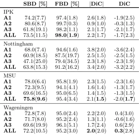
Table 2: Segmentation and counting results on the train-ing set. Average values are shown for metrics described in Section 3 and in parenthesis standard deviation. ‘ALL’ denotes the average (and standard deviation) among the three datasets for each method. Other shorthands and abbreviations as defined in text (Sections 3 and 6).

SBD [%] FBD [%] |DiC| DiC IPK

A1 74.2(7.7) 97.4(1.8) 2.6(1.8) -1.9(2.5) A2 80.6(8.7) 99.7(0.3) 0.9(1.0) -0.3(1.3) A3 61.8(19.1) 98.2(1.1) 2.1(1.7) -2.1(1.7) ALL 73.5(11.5) 98.0(1.9) 2.2(1.7) -1.7(2.3)

Nottingham

A1 68.0(7.4) 94.6(1.6) 3.8(2.0) -3.6(2.4) A2 60.9(18.5) 87.5(19.7) 2.5(1.5) -2.5(1.5) A3 47.1(25.0) 79.4(34.5) 2.3(1.8) -2.3(1.9) ALL 63.8(15.3) 91.2(16.2) 3.4(2.0) -3.2(2.2)

MSU

A1 78.0(6.4) 95.8(1.9) 2.3(1.5) -2.3(1.6) A2 72.3(9.5) 94.1(4.1) 1.6(1.4) -1.3(1.7) A3 69.6(16.5) 95.0(6.5) 1.4(1.5) -1.3(1.5) ALL 75.8(9.6) 95.4(3.4) 2.1(1.5) -2.0(1.7)

Wageningen

A1 72.8(7.8) 95.0(2.4) 2.2(2.0) 0.4(3.0) A2 71.7(8.0) 95.2(2.4) 1.3(1.1) -0.6(1.6) A3 69.6(19.9) 96.1(5.1) 1.7(2.4) 0.6(2.9) ALL 72.2(10.5) 95.2(3.0) 2.0(2.0) 0.3(2.8)

Table 3: Segmentation and counting results on the test-ing set. Shorthands and abbreviations as in Table 2.

SBD [%] FBD [%] |DiC| DiC IPK

A1 74.4(4.3) 97.0(0.8) 2.2(1.3) -1.8(1.8) A2 76.9(7.6) 96.3(1.7) 1.2(1.3) -1.0(1.5) A3 53.3(20.2) 94.1(13.3) 2.8(2.5) -2.0(3.2) ALL 62.6(19.0) 95.3(10.1) 2.4(2.1) -1.9(2.7)

Nottingham

A1 68.3(6.3) 95.3(1.1) 3.8(1.9) -3.5(2.4) A2 71.3(9.6) 93.0(4.2) 1.9(1.7) -1.9(1.7) A3 51.6(16.2) 90.7(20.4) 2.5(2.4) -1.9(2.9) ALL 59.0(15.6) 92.5(15.6) 2.9(2.3) -2.4(2.8)

MSU

A1 66.7(7.6) 94.0(1.9) 2.5(1.5) -2.5(1.5) A2 66.6(7.9) 87.7(3.6) 2.0(1.5) -2.0(1.5) A3 59.2(17.8) 95.0(5.2) 2.3(1.9) -2.3(1.9) ALL 62.4(14.8) 94.0(4.7) 2.4(1.7) -2.3(1.8)

Wageningen

A1 71.1(6.2) 94.7(1.5) 2.2(1.6) 1.3(2.4) A2 75.7(8.4) 95.1(2.0) 0.4(0.5) -0.2(0.7) A3 57.6(24.8) 89.5(22.3) 3.0(4.9) 1.8(5.5) ALL 63.8(20.5) 91.7(17.0) 2.5(3.9) 1.5(4.4)

methods merge leaves: this lowers SBD scores but affects count numbers even more critically. Other methods (e.g., Wageningen) tend to over-segment and consider other parts as leaves (see for example the second image of ‘A1’ in Figure 9), which sometimes leads to over counting.

Number of leaves

0 5 10 15 20

DiC

-15 -10 -5 0 5 10 15

A1 A2 A3

(a) IPK

Number of leaves

0 5 10 15 20

DiC

-15 -10 -5 0 5 10 15

A1 A2 A3

(b) Nottingham

Number of leaves

0 5 10 15 20

DiC

-15 -10 -5 0 5 10 15

A1 A2 A3

(c) MSU

Number of leaves

0 5 10 15 20

DiC

-15 -10 -5 0 5 10 15

A1 A2 A3

(d) Wageningen

Fig. 11: For each method scatters of number of leaves in ground-truth vs. Difference in Count (DiC) are shown for the testing set. Each dataset is color coded differently. Also, lines of average and average ±one standard devi-ation of DiC are shown, as solid and dashed blue lines, respectively.

These misestimations are evident throughout train-ing and testtrain-ing sets (cf. Tables 2 and 3). Stepptrain-ing away from the summary statistics of the tables, over and under estimation are readily apparent in Figure 11. All algo-rithms present counting outliers, where MSU yields the least count variability, even though with a clear under-estimation. The mean DiC of Wageningen is the closest to zero, albeit featuring the highest variances. We also observe that DiC slopes down as the number of leaves increases, particularly in the case of ‘A3’.

7.3 Plant growth and complexity

Plants are complex and dynamic organisms that grow in time, and move throughout the day and night. They grow differentially, with younger leaves growing faster than mature ones. Therefore, per leaf growth is a bet-ter phenotyping trait when evaluating growth regulation and stress situations. As they grow, new leaves appear and plant complexity changes: in tobacco more leaves overlap and exhibit higher nastic movements; and in Ara-bidopsis younger leaves emerge, overlapping other more mature ones.

Number of leaves

0 2 4 6 8 10 12 14

SBD

0 10 20 30 40 50 60 70 80 90 100

IPK Nottingham MSU Wageningen

Fig. 12: Effect of plant complexity (measured as number of leaves) on leaf segmentation accuracy, i.e., SBD, for ‘A3’. Each method is marker coded separately.

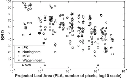
Projected Leaf Area (PLA, number of pixels, log10 scale)

103 ₁₀4 ₁₀5 ₁₀6 ₁₀7

SBD

0 10 20 30 40 50 60 70 80 90 100

IPK Nottingham MSU Wageningen

Fig. 13: Effect of plant size, measured as number of plant pixels in ground truth, (Projected Leaf Area) on leaf segmentation accuracy, i.e., SBD, for ‘A3’. Each method is marker coded separately.

Using classical growth stages, which rely on leaf count as a marker of growth, the downwards slope seen in Fig-ure 11 could be attributed to growth. This is more clear in Figure 12, where we see that with more leaves, leaf segmentation accuracy (SBD) also decreases.

Even if we consider plant size (measured as projected leaf area, i.e., the size of the plant in ground-truth, ob-tained as the union of all leaf masks), we observe a de-creasing trend in SBD for each method with plant size, see Figure 13. Observe the large variability in SBD when plants are smaller. Even isolating it to a single method we see that when plants are small, depending on the plant’s leaf arrangement, variability is extremely high: either good (close to 0.8) or rather low SBD values are obtained.

7.4 Effect of foreground segmentation accuracy

In Figure 14 we plot FBD vs. SBD for each method pool-ing the testpool-ing data together. We see that high SBD can only be achieved when FBD is also high; but obtain-ing a high FBD is not at all a guarantee for good leaf

FBD

60 65 70 75 80 85 90 95 100

SBD

0 10 20 30 40 50 60 70 80 90 100

IPK Nottingham MSU Wageningen

Fig. 14: Effect of plant vs. leaf segmentation accuracy (FBD vs. SBD). Each method is marker coded sepa-rately. Data from all datasets pooled together; results with FBD<0.6 are omitted for clarity.

segmentation (i.e., a high SBD) since we observe large variability in SBD even when FBD is high.

This prompted us to evaluate the performance of the leaf segmentation part isolating it from errors in the plant (foreground) segmentation step. Thus, we asked participants to submit results on the training set assum-ing that also a foreground (plant) mask is given (as ob-tained by the union of leaf masks), effectively not requir-ing a plant segmentation step.

Naturally, all methods benefit when the ground-truth plant segmentation is used: compare SBD, DiC, and|DiC|

Table 4: Segmentation and counting results on the train-ing setassuming foreground segmentation known. Short-hands and abbreviations as in Table 2.

SBD [%] |DiC| DiC IPK

A1 79.1(5.5) 2.1(1.4) -1.9(1.7) A2 80.7(10.8) 1.2(1.3) -1.1(1.4) A3 71.0(20.6) 1.8(1.8) -1.8(1.8) ALL 78.2(10.4) 1.9(1.5) -1.8(1.7)

Nottingham

A1 71.0(7.2) 4.4(1.7) -4.4(1.7) A2 66.5(21.6) 2.5(1.5) -2.7(1.5) A3 59.5(11.3) 2.4(1.3) -2.4(1.3) ALL 68.6(12.1) 3.9(1.9) -3.9(1.9)

MSU

A1 78.5(5.5) 2.5(1.4) -2.5(1.4) A2 77.4(8.1) 1.6(1.3) -0.9(1.9) A3 76.1(14.1) 1.2(1.2) -1.1(1.2) ALL 78.0(7.8) 2.2(1.4) -2.0(1.6)

Wageningen

A1 77.3(4.9) 1.5(1.3) -0.3(2.0) A2 75.5(8.0) 1.3(1.3) -0.9(1.6) A3 76.5(14.6) 1.4(1.3) -1.3(1.4) ALL 76.9(7.6) 1.5(1.3) -0.5(1.9)

7.5Performance under blinded shape based metrics

Most of the metrics we adopted for the challenge rely on segmentation and area based measurements (cf. Sec-tion 3). It is thus of interest to see how the methods per-form on metrics that evaluate boundary accuracy and reward methods that best preserve leaf shape. Notice that these metrics were not available to the participants, so methods have not been optimized for such metrics. For brevity we present results on the testing set only.

We adopt two metrics, based respectively on the Mod-ified Hausdorff Distance (MHD) [19] and Pratt’s Figure of Merit (FoM) [45], to compare point setsAandB de-noting leaf object boundaries.

The Modified Hausdorff Distance (MHD) [20] mea-sures the displacement of object boundaries as the aver-age of all the distances from a point inAto the closest point in B. With

D(A,B) = 1

|A| X

p∈A min

q∈Bkp−qk, (5)

wherek · kis the Euclidean distance, MHD is defined as:

MHD(A,B) = max{D(A,B), D(B,A)}. (6)

This metric is known to be suitable for comparing tem-plate shapes with targets [20]. It prioritizes leaf boundary accuracy, being relevant for shape-based leaf recognition purposes.

Pratt’s Figure of Merit (FoM) [45] was introduced in the context of edge detection and penalizes missing or

displaced points between actual (A) and ideal (I) bound-aries:

FoM(A,I) = 1 max{|A|,|I|}

|A|

X

i=1 1 1 +αd2

i

, (7)

whereα= 1/9 is a scaling constant penalizing boundary offset, anddiis the distance between an actual boundary point and the nearest ideal boundary point.

Let Bar _{and B}gt _{be sets of leaf object boundaries} extracted from leaf segmentation masks Lar _{and L}gt_, respectively, whereBar _{is the algorithmic result andB}gt is the ground truth. To evaluate how well leaf object shape and boundaries are preserved, and to follow the spirit of SBD defined in Section 3, we use:

– Symmetric Best Hausdorff (SBH), the symmetric average MHD among all object (leaf) boundaries, where for each input label the ground truth label yielding minimum MHD is used for averaging. Best Hausdorff (BH) is defined as:

BH(Ba, Bb) =

     

    

p

w2_+h2

if either

Ba=∅or

Bb=∅

1 M

M

X

i=1 min

1≤j≤NMHD(B a

i, B

b

j) otherwise

(8)

whereBa

i for 1≤i≤M and Bjb for 1≤j ≤N are point sets corresponding to the boundaries, respec-tively,Ba _{and B}b_{, of leaf object segments belonging} to leaf segmentationsLa _andLb_{;wandhdenote,} re-spectively, width and height of the image containing the leaf object. SBH is then:

SBH(Bar, Bgt) =

maxBH(Bar, Bgt), BH(Bgt, Bar) . (9)

SBH is expressed in units of length (e.g., pixels or mil-limetres) and is 0 for perfectly matching boundaries. IfBar _{is empty, SBH is equal to the image diagonal} (i.e., the greatest possible distance between any two points).

– Best Figure of Merit (BFoM), the average FoM a-mong all leaf objects, where for each input label the ground truth label yielding maximum FoM is used for averaging.

BFoM(Bar, Bgt) =

1 M

M

X

i=1 max

1≤j≤NFoM(B ar

i , B

gt

j ), (10)

Table 5: Segmentation results on the testing set with respect to leaf shape. Shorthands and abbreviations as in Table 2. Notice that for SBH lower is better whereas for BFoM higher is better.

SBH [pix] SBH [mm] BFoM [%]

IPK

A1 9.2(3.2) 1.54(0.53) 62.6(7.3)

A2 6.9(3.6) 1.15(0.60) 66.9(8.1)

A3 174.9(442.8) 7.00(17.7) 41.9(17.3)

ALL 103.6(343.5) 4.62(13.4) 51.1(17.6)

Nottingham

A1 13.0(5.9) 2.17(0.99) 58.7(9.0)

A2 9.3(5.7) 1.55(0.95) 62.3(7.4)

A3 193.6(589.7) 7.74(23.6) 49.2(21.8)

ALL 115.8(453.1) 5.30(17.8) 53.6(18.1)

MSU

A1 13.3(5.6) 2.22(0.94) 50.9(10.3)

A2 10.0(6.3) 1.67(1.05) 52.0(12.2)

A3 81.1(105.6) 3.24(4.22) 46.5(19.0)

ALL 51.7(86.6) 2.76(3.25) 48.5(16.1)

Wageningen

A1 13.0(5.6) 2.17(0.94) 54.1(9.1)

A2 10.2(7.8) 1.70(1.30) 61.1(9.7)

A3 109.1(227.0) 4.36(9.08) 43.7(26.7)

ALL 67.7(177.6) 3.38(6.90) 48.8(21.8)

In Table 5 we see the results on the testing set using these metrics. SBH values vary strongly between dataset ‘A3’ and the other two (‘A1’ and ‘A2’). This indicates an issue when using SBH with images of different size. Being a distance, SBH given in pixel depends on resolution. We therefore also give it in object dimensions i.e. mm, even though object resolution depends on (the non-constant) local object distance from the camera. Overall, MSU re-ports best average performance according to SBH (al-though this result is largely influenced by the ‘A3’ data-set) with IPK performing best on ‘A1’ and ‘A2’. With respect to BFoM, IPK again performs best on ‘A1’ and ‘A2’, while Nottingham outperforms the other methods on ‘A3’. Interestingly, the overall ranking of the methods according to the two metrics is opposite.

MSU exhibits lower variance compared to IPK, Not-tingham and Wageningen, since the latter methods in-clude some empty segmentations (i.e., no leaf objects found) in the testing results, which in BFoM evaluate to 0 and in SBH to the image diagonal length. This situation occurs for some images of very small plants, which are probably missed in the segmentation step of the methods.

7.6 Differences among datasets

Although the tobacco dataset, ‘A3’, has higher resolution and leaf boundaries are more evident, rich shape varia-tion and large overlap among leaves challenge all meth-ods: almost all achieve lower performance compared to

‘A1’ and ‘A2’ (Tables 2 and 3). Even the variability in ac-curacy increases for ‘A3’. The MSU algorithm shows the least variability among datasets probably due to the fact that it uses templates (rotated and scaled). As such it can adapt better to different shape variability and heav-ier occlusions and is more robust to plant segmentation errors. It is also due to the reliance on an edge map to fit the templates: on ‘A3’ it can be estimated more reliably compared to ‘A1’ and ‘A2’, where some images can be blurry (due to larger field of view) and resolution is lower. However, when foreground is known (Table 4) variability of the Wageningen solution also becomes lower between datasets.

‘A2’ does contain images from different mutants but shows different image background with respect to ‘A1’ (black textured tray vs. red smoother tray). When plant mask is assumed known,SBDresults on the training set show (Table 4) thatNottingham, MSU, and Wageningen still do better in ‘A1’ than in ‘A2’, and all methods show higher variances in ‘A2’ than in ‘A1’.So it might appear that different mutants play a role; however, this result is not conclusive since ‘A2’ has fewer images than ‘A1’. In fact, a simple unpaired t-test between SBD in ‘A1’ and ‘A2’ shows no statistical difference (for any of the methods).

We should point out that both Nottingham and Wa-geningen use the same mechanism to segment leaves: a watershed on the distance (from the boundary) map. However, Nottingham relies on finding first centers and then using those as seeds for leaf segmentation, while Wageningen obtains an over-segmentation and then mer-ges parts using a threshold on the basins. Their perfor-mance difference due to this algorithm selection becomes apparent when comparing results with given foreground segmentation (Table 2). We see that the Wageningen al-gorithm does better compared to the Nottingham solu-tion. We conclude that finding suitable seeds for segmen-tation is hard and further, comparing Figure 10, that this is true especially for small leaves. On the other hand, it appears that the Wageningen algorithm finds a suitable threshold for merging according to the dataset.

7.7Discussions on Experimental Work

rela-tively good accuracy, although methods that obtain high average and low variance should be sought-after.

On the other hand, measuring individual leaf growth on the basis of leaf segmentations shows currently low ac-curacy. The algorithms presented here show an average accuracy of62.0% (best 63.8%, see Table 3)in segment-ing a leaf and almost always miss leaves, particularly un-der heavy occlusions among leaves and when both small (young) and larger (mature) leaves are present within the same plant. SBD does not necessarily capture that, but is evident when analyzing leaf size vs. Dice accu-racy and leaf counts. In several occasions leaf count is off (missing several leaves) and frequently the algorithms are segmenting as leaves disconnected leaf parts (partic-ularly their stems).10

Several approaches (IPK and Nottingham) assume that once a center of a leaf is found that segmentation can be obtained by region growing methods. Naturally, when leaves heavily overlap they do miss to identify the cen-ters (and find less leaf cencen-ters than in the ground truth), which holds for both rosette plants considered here. Also when image contrast is not ideal, lack of discernible edges leads to a misestimation of leaf boundaries. This is par-ticularly evident in the Arabidopsis data (‘A1’ and ‘A2’) and affects approaches that rely on edge information (MSU). The tobacco dataset (‘A3’) being high resolu-tion does offer superior contrast, but the amount of over-lap and shape variation is significant leading to under-performance for most of the algorithms.

We also investigate performance on leaf boundaries using SBH and BFoM (cf. Section 7.5). SBH penalizes boundary regions being far away from where they should be, whereas BFoM acknowledges boundaries being in the right position. Thus, from a shape sensitive application viewpoint, low SBH is needed if boundary outliers lead to low performance, whereas high BFoM is advisable if an algorithm is robust against outliers. When choosing from the solutions presented here, a trade-off needs to be found, as high BFoM (good) comes with high SBH (bad) and vice versa.

Evident by the meta-analysis of all results is the ef-fect of plant complexity (due to plant age, mutant, or treatment) on algorithmic accuracy. Leaf segmentation accuracy decreases with larger leaf count (Figure 12), using leaf count as a proxy for maturity [15]. This is expected: as the plant grows and becomes more com-plex, more leaves and higher overlap between young and mature leaves are present. Overall, most methods face greater difficulties in detecting and segmenting smaller (younger) leaves (Figure 10), most likely not due to their size, but overlap: they tend to grow on top of more ma-ture leaves.

Moving forward, no approach here relies on learning a model on the basis of the training data to obtain leaf

10 _{This indicates that additional (possibly tailored)} evalua-tion metrics may be necessary, although our testing with some common in the literature did not yield any improvement.

segmentations and this might lead to promising algo-rithms in the future. Interestingly, some of our findings on learning to count leaves do show that leaf count can be estimated without segmentation [22]. However, indi-vidual and accurate leaf segmentation is still important: for example, studying individual leaf growth, tracking leaf position and orientation, classifying young from old leaves, and others.

One alternative which changes the problem defini-tion and may reduce complexity is to provide addidefini-tional data such as temporal (time-lapse images) and/or depth (stereo and multiview imagery) information. The former can be used for better leaf segmentation, e.g. via joint segmentation-tracking approaches [60, 61]. Both types of information will help in resolving occlusions and obtain-ing better boundaries. Currently, such data are not pub-licly available but we are working to release such curated datasets and dedicated annotation tools to the commu-nity[38, 37].

8Conclusion and Outlook

This paper presents a collation study of a variety of leaf segmentation algorithms as tested within the confines of a common dataset and a true scientific challenge: the Leaf Segmentation Challenge of CVPPP 2014. This is the first of such challenges in the context of plant phe-notyping and we believe that such formats will help ad-vance the state of the art of this societally important application of machine vision.

Having annotated data in the public domain is ex-tremely beneficial and this is one of the greatest out-comes of this work. They can be used not only to moti-vate and enlist interest from other communities but also to support future challenges (similar to this one). We all believe that here is the future: it is via such challenges that the state of the art advances rapidly and new chal-lenges for 2015 have already been publicized.11_However, these challenges should happen in a rolling fashion, year-round, with leader boards and automated evaluation sys-tems. It is for this reason that we are considering a web-based system, e.g., similar in concept to Codalab,12 _for people to submit results but also deposit new annotated datasets. This has been proven useful in other areas of computer vision (consider for example PASCAL VOC [21]) and it will benefit also plant phenotyping.

In summary, the better we can “see” the plant-organs via new computer vision algorithms evaluated on a com-mon dataset and collectively presented, the better phe-notyping we do, and the higher societal impact.

11 _{See the 2015 LSC and the new Leaf Counting Challenge of} CVPPP 2015 at BMVC (http://www.plant-phenotyping. org/CVPPP2015).

12