The Mechatronics System Control Quality
Analysis Using Simulink and GUI in Matlab
M. Juhás, B. Juhásová, and P. Mydlo
Abstract—In this contribution is presented study of flexible mechatronics system control quality analysis. Control system is designed by various standard and advanced methods. The different criteria for quality evaluation are used. The Matlab – Simulink simulation model in conjunction with Matlab GUI is used for experiments realization.
Index Terms—control quality, Matlab GUI, mechatronics system control, Simulink
I. INTRODUCTION
T
HE contribution deals with flexible mechatronics system control quality analysis by the Simulink tool and with GUI utilization created in the Matlab. The impulse is ongoing necessity of further advancement of electric drives containing elements with different types of parasitic effects control methods, in this case flexible connection between an actuator and a load. There are different methods of mechatronics system control design analyzed in this article. The control quality is advised on base of local criterion as well as integral quality criterion.II. CONTROLLED SYSTEM MODEL
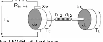
The permanent magnet synchronous motor (PMSM) with flexible coupling is chosen as analyzed mechatronics system. A special type of PMSM with the high torsion moment by the relatively low evolves – torque motor, was analyzed.
[image:1.595.47.225.605.678.2]If the inertia of the transmission mechanisms is small compared to the motor and load, the flexible coupling between the motor and load can be treated as a two-mass motor/load system, as shown in Fig. 1. [2, 5, 6]
Fig. 1 PMSM with flexible join
Manuscript received June 20, 2012; revised July 22, 2012.
M. Juhás is with the Institute of AIAM FMST SUT in Trnava, Hajdóczyho 1, 917 01 Trnava, Slovak Republic (phone: +421 918 646 021; e-mail: [email protected]).
B. Juhásová is with the Institute of AIAM FMST SUT in Trnava, Hajdóczyho 1, 917 01 Trnava, Slovak Republic (e-mail: [email protected]).
P. Mydlo is with the Institute of AIAM FMST SUT in Trnava, Hajdóczyho 1, 917 01 Trnava, Slovak Republic (e-mail: [email protected]).
TABLEI
ANALYZED SYSTEM PARAMETERS
Parameter Unit Description Value
Ra Ω armature current 0.02
La mH resistance and inductance of armature winding 100
cΦ Nm/A torque constant 0.3
JM kg/m2 inertia of the motor rotor 10 JL kg/m2 inertia of the load 60 b12 Nms damping of the transmission 0.1 d12 Nm spring constant of the transmission 4
kTM - converter gain 1
TTM - converter time constant 2 The control system design was based on idealized condition where the infinitely rigid connection was considered instead of flexible connection between actuator and a load. This condition is described as
L
M J
J
J= + (1)
Oversimplified model of system as transfer function of this adjusted mechatronics system has a form
2 a L M 2 a L M PMSM
c s R ) J J ( s L ) J J (
c )
s ( G
Φ + +
+ +
Φ
= (2)
A spurious effects caused by resonant frequency and antiresonant frequency occurrence in the flexible connection were eliminated by double notch filter [7, 9] in form
1 s 2 s 1
1 s 2 s 1
) s ( G
a a 2 2
a
r r 2 2
r filter
+ ω
ξ + ⎟⎟ ⎠ ⎞ ⎜⎜ ⎝ ⎛
ω
+ ω
ξ + ⎟⎟ ⎠ ⎞ ⎜⎜ ⎝ ⎛
ω
= (3)
where resonance:
L M
L M 12 r
J J
J J
d +
=
ω (4)
resonance dumping:
L M 1 12
L M 12 r
J J d
J J 2
b +
=
ξ (5)
antiresonance:
L 12 a
J d =
ω (6)
antiresonance dumping:
L 12 12 a
J d 2
b =
ξ (7)
III. CONTROL SYSTEM DESIGN AND CONTROL SYSTEM MODEL
For control system design was applied different methods. [1, 3, 4, 8] Classical feedback control has been designed by
--Modulus Optimum Method --Method of Inverse Dynamics
Next, the combination of classical feedback control and one of intelligent control methods has been applied
--Fuzzy controller
An advanced control method in form of cascade control with utilization
--2x Modulus Optimum Method
--Modulus Optimum Method and Symmetric Optimum Criterion
was also used.
A. Feedback control of angular velocity
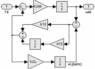
The simulation was performed by simulation model (Fig. 2) [10] consists of
--controlled system – actuator electrical part (Fig. 3) and flexible join of actuator with load (Fig. 4) --controller GR(s)
[image:2.595.118.546.27.774.2]--double notch filter
[image:2.595.48.207.528.644.2]Fig. 2 Simulation model of angular velocity feedback control
Fig. 3 Analyzed system simulation model of electrical part
Fig. 4 Analyzed system simulation model of flexible join
PI controller – Naslin method
For controller of PI type in form s r r ) s ( G 1 0
R = + − (8)
is the closed control loop in form
1 0
2
3 1.4s (00.09 0.31r )s 0.3r
s 7 r 3 . 0 s r 3 . 0 ) s ( Gc − − + + + + +
= (9)
According this, for and maximum overshooting 5% following a Naslin method are valid inequalities
2 = α : a a
a12≥α 0 2 (0.09+0.3r0)2=2*0.3r−1*1.4 (10)
: a a a2 1 3
2≥α 1.42=2*(0.09+0.3r0)*7 (11)
For PI controller coefficients calculation is used a boundary state – equality and the resulting values are
TABLEII
PI(NASLIN)CONTROLLER PARAMETERS
Parameter Value r0 0.1667
r–1 0.0233
PID controller – Modulus Optimum Method
For controller of PID type in form s r s r r ) s (
GR = 0+ −1+ 1
(12) has an opened control loop form
s 09 . 0 s 4 . 1 s 7 r 3 . 0 s r 3 . 0 s r 3 . 0 ) s (
Go 3 20 1
2 1 + + + + = − (13) Following an assumption that ideal closed control system
transfer function has a value approaching to one, the equation involving real part of open control loop frequency response has form
2 4
6 0 1
2 0 1 4 0081 . 0 7 . 0 49 ) r 42 . 0 r 027 . 0 ( ) r 1 . 2 r 42 . 0 ( ) s ( Go ω + ω + ω − ω + − ω = − 5 . 0 ) s (
Go =− (14)
The coefficients of PID controller are solved based on equations system in matrix form solution
⎥ ⎥ ⎥ ⎦ ⎤ ⎢ ⎢ ⎢ ⎣ ⎡ − = ⎥ ⎥ ⎥ ⎦ ⎤ ⎢ ⎢ ⎢ ⎣ ⎡ ⎥ ⎥ ⎥ ⎦ ⎤ ⎢ ⎢ ⎢ ⎣ ⎡ − − − 49 7 . 0 0081 . 0 5 . 0 r r r 0 0 0 42 . 0 1 . 2 0 0 027 . 0 42 . 0 1 0 1 (15)
The coefficients of PID controller designed by Modulus Optimum Method are
TABLEIII
PID(MOM)CONTROLLER PARAMETERS
Parameter Value r0 0.1602
r–1 0.0199
r1 –0.0323
PID controller – Method of Inverse Dynamics
For possibility to calculate controller coefficients by Method of Inverse Dynamics was transfer function of an actuator rigidly connected with a load modified to the form 1 s T 2 s T K 09 . 0 s 4 . 1 s 7 3 . 0 ) s ( G 0 2 2 0 2 PMSM + ξ + = + +
= (16)
where 09 . 0 / 3 . 0
K= ;T0= 7/0.09;
0 T * 2 * 09 . 0 4 . 1 =
ξ (17)
The coefficients of PID controller in form ) s T s T 1 ( P ) s (
GR = + i + d (18)
are for defined time constant Tw=0.1 calculated
according to equations
0
i 2 T
T = ξ ; ξ =
2 T Td 0;
w i
KT T
P= (19)
[image:2.595.320.550.600.760.2]TABLEIV
PID(MID)CONTROLLER PARAMETERS
Parameter Value P 46.6713 Ti 15.5556
Td 5
Fuzzy control
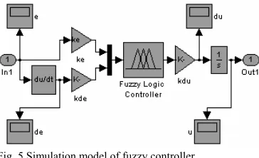
The fuzzy controller was designed by experimental variation of ke, kde and kdu coefficients based on ITAE
[image:3.595.102.227.54.114.2]quality criteria tracking and evaluation. The simulation model of fuzzy controller, which was used in this simulation experiment, is shown in Fig. 5.
Fig. 5 Simulation model of fuzzy controller
The resultant values of fuzzy controller are TABLEV
PD(FUZZY)CONTROLLER PARAMETERS
Parameter Value ke 0.0016
kde 0.0165
kdu 787.8
B. Cascade control
The most frequently used control structure in the controlled drives is the cascade control. In the case of speed control of PMSM are using two loops namely
--current (eventually torque) loop --speed loop
Fig. 6 Simulation model of PMSM cascade control
Current controller
The tuning method based on the Modulus Optimum optimization criterion was used for current controller design.
According to this criterion was specified PI controller in form
s Ti
1 s Ti k R
PI PI PI
PI= + (20)
with coefficients defined as
a TM a
a PI TM PI
PI ;Ti L /R ;k k /R
kT 2
Ti
k = = = (21)
The coefficients of cascade control subordinate PI current controller designed by Modulus Optimum Method are
TABLEVI
PI(MOM)CURRENT CONTROLLER PARAMETERS
Parameter Value kPI 0.025
TiPI 5
Speed controller I
The tuning method based on the Symmetric Optimum Criterion was used for first version of speed controller design.
According to the Symmetric Optimum Criterion was specified PID controller in form:
s Td s Ti k
RPID = PID+ PID + PID (22)
with coefficients defined as
(
)
TM 2 PID
2 TM PID
2 TM TM PID
T c 2
J Td
; T c 8
J Ti
; T c 8
J T 4 J k
φ =
φ = φ
+ =
(23)
The coefficients of cascade control master PID angular velocity controller designed by Symmetric Optimum Criterion are
TABLEVII
PID(SOC)CURRENT CONTROLLER PARAMETERS
Parameter Value kPID 568.75
TiPID 7.2917
TdPID 4083.3
Speed controller II
The tuning method based on the Modulus Optimum criterion was used for second version of speed controller design.
According to the Modulus Optimum criterion was specified PD controller in form:
(
1 Td s)
k
RPD = PI + PI (24)
with coefficients defined as
TM PI
TM
PI ;Td 2T
T J c 2
1
k =
φ
= (25)
The coefficients of cascade control master PD angular velocity controller designed by Modulus Optimum Method are
TABLEVIII
PD(MOM)CURRENT CONTROLLER PARAMETERS
Parameter Value kPD 58.3333
TdPD 4
IV. GRAPHICAL USER INTERFACE FOR QUALITY ANALYSIS
[image:3.595.49.231.204.315.2]application utilizes simulation and analysis of created simulation models to view various qualitative indicators. It also allows analyzing influence of elimination element – double notch filter application on control process quality increase.
Fig. 7 GUI for PMSM Control Quality Analysis
V. ANALYSIS RESULTS
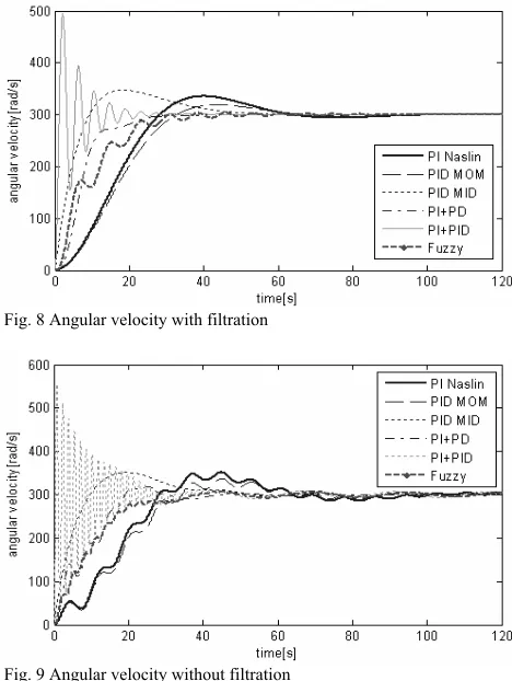
[image:4.595.46.282.117.280.2]The plots of angular velocity of particular simulation experiments are displayed extra for enabled (Fig. 8) and extra for disabled (Fig. 9) parasitic frequency filtration.
Fig. 8 Angular velocity with filtration
Fig. 9 Angular velocity without filtration
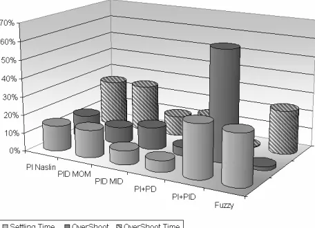
The quality of control process has been evaluated based on local criteria of quality
--Settling Time --OverShoot --OverShoot Time
as well as based on integral criteria of quality for control error space, acquired through the simulation subsystem [10] shown in Fig. 10.
--Integral Square Error (ISE) --Integral Time Square Error (ITSE) --Integral Absolute Error (IAE) --Integral Time Absolute Error (ITAE)
Fig. 10 Simulation subsystem for integral criteria measurement The results of experiments, consisting of evaluating of different quality markers for different methods of flexible mechatronics system control design are shown in TABLE IX
TABLEIX SIMULATION RESULTS
[image:4.595.316.550.356.509.2]Reached results were represented in graphical form (Fig. 11, Fig. 12, Fig. 13 and Fig. 14) because of analyses requirement. Graphical representation does not contain absolute numerical expression of results, but because of comparability they were transformed to percentage representation of specific part relative to entirety.
[image:4.595.45.279.366.677.2] [image:4.595.317.548.594.761.2]Fig. 12 Simulation results – Integral criteria of quality without filtration
Fig. 13 Simulation results – Local criteria of quality with filtration
Fig. 14 Simulation results – Local criteria of quality without filtration
VI. CONCLUSION
The set of experiments, consist of simulation of flexible mechatronics system with control system designed by different methods, has been performed. The quality of control process was evaluated based on different markers. According to achieved results is possible to state, that:
--for control design necessity is possible to use a substitution of infinitely rigid join instead of flexible join in the concurrency with utilization of filter for flexible system antiresonant and resonant frequency;
--classical principles of control design (Naslin, MOM)
are of advantage in term of local criterion especially by using them without filtering of parasitic elements, but according to quality integral criterion is their application markedly inept;
--according to integral criteria, as an optimal method for control design wears the cascade control with PI current controller and PID angular velocity controller, which is however at least advantageous in the term of maximal overshooting value;
--usage of advanced control methods, represented by fuzzy control in this case considering dynamics and system structure wears as disadvantageous;
--after evaluation of combination of all indicators is possible to assert, that the one of optimal methods of flexible mechatronics system control design is possible to consider the classical design method - method of inverse dynamics and advanced method - cascade control contains combination of PI current controller and PD angular velocity controller. These two methods show signs of robustness furthermore, in terms of unacceptable frequencies elimination without using of supplementary filter too.
REFERENCES
[1] J. Balátě, “Automatické řízení,” BEN – technická literatura, Praha, 2003
[2] D.A. Bradley, D. Dawson, N.C. Burd, A.J. Loader, “Mechatronics,” Chapman & Hall, London, 1991. ISBN 0-412-58290-2.
[3] I. Švarc, R. Matoušek, M. Šeda and M. Vítečková, “Automatické řízení,“ Akademické nakladatelství CERM, s.r.o. Brno, 2011 [4] M. Vítečková, A. Víteček, “Modulus optimum for digital
controllers,” Acta Montanistica Slovaca, 2003, vol. 8, no. 4, pp. 214 – 216.
[5] S. Vukosavic, M. Stojic, “Suppression of Torsional Oscillations in a High-Performance Speed Servo Drive,” IEEE Trans. on Industrial Electronics, vol. 45, pp. 108-117, Jan. 1998.
[6] J. Vittek, P. Briš, P. Makyš, M. Štulrajter and V. Vavruš, “Control of Flexible Drive with PMSM employing Forced Dynamics,” 13th EPE-PEMC 2008, pp. 2219-2226. IEEE 978-1-4244-1742-1. [7] J. Jovankovič, M. Žalman, “Mechatronické pohybové systémy
(2),” AT&P journal, 2006, vol. XIII, no. 3, pp. 73 – 74. ISSN 1335-2237
[8] G. Ellis, “Control system design guide,” San Diego: Elsevier Academic Press, 2004. 464 pp. ISBN 0-12-237461-4
[9] J. Kalous, C. Kratochvíl and P. Heriban, “Dynamics of Rotary Electromechanical Drives,” ÚT AVČR – Centrum mechatroniky, Brno, 2007. ISBN: 80-214-3340-X.
[10] MathWorks. (2012, May 20). Simulink [Online]. Available: http://www.mathworks.com/products/simulink/
[image:5.595.49.277.441.606.2]