Erosion Potential Method (Gavrilović method) sensitivity analysis

Erosion Potential Method (Gavrilović Method)

Sensitivity Analysis

Nevena DRAGIČEVIĆ*, Barbara KARLEUŠA and Nevenka OŽANIĆ

1_{Department of Hydrotechnics and Geotechnics, Faculty of Civil Engineering,}

University of Rijeka, Rijeka, Croatia *Corresponding author: [email protected]

Abstract

Dragičević N., Karleuša B., Ožanić N. (2017): Erosion Potential Method (Gavrilović method) sensitivity analysis. Soil & Water Res., 12: 51−59.

In recent decades, various methods for erosion intensity and sediment production assessment have been de-veloped. The necessity for better model performance has led to the more frequent application of the method sensitivity and uncertainty assessments in order to decrease errors that arise from the model concept and its main assumptions. The analysis presented in this paper refers to the application of the Gavrilović method (Ero-sion Potential Method), an empirical and semi-quantitative method that can estimate the amount of sediment production and sediment transport as well as the erosion intensity and indicate the areas potentially threatened by erosion. The emphasis in this paper is given upon the method sensitivity analysis that has not previously been conducted for the Gavrilović method. The sensitivity analysis was conducted for fourteen different parameters included in the method, all in relation to different model outputs. Each parameter was perceived and discussed individually in relation to its effect upon the method outputs, and ranked into categories depending on their influence on one or more model outputs. The objective of the analysis was to explore the constraints of the Gavrilović method and the method response to changes deriving from the each individual parameter in an at-tempt to provide a better understanding of the method, the weight and the contribution of each parameter in the overall method. The parameters that could potentially be used in future research, for method modification and calibration in areas with different catchment characteristics (e.g. climate, geological, etc.) were identified. The most sensitive model parameters resulting from conducted sensitivity analysis for the Gavrilović method are also those considered to be significant in the scientific literature on erosion. The Gavrilović method sensitivity analysis has been done on a case study for the Dubracina catchment area, Croatia.

Keywords: erosion assessment; erosion intensity; input parameters; method sensitivity; sediment production

The need for information on soil erosion (Merritt et al. 2003), at temporal and spatial scales describing the sediment pattern throughout the catchment and its associated quantities, is increasing due to various demands from stakeholders and decision makers in spatial as well as soil and water conservation plan-ning. In recent decades, many methods for erosion intensity and sediment production assessment have been developed. The necessity for better model per-formance has led to more frequent application of the method sensitivity and uncertainty assessments in order to decrease errors that arise from the model

each one or in a set of input parameters (Loucks & Van Beck 2005; Morgan 2005) and quantitatively evaluates the influence of input parameters to model outcome. Numerous studies (e.g. Jetten et al. 1999, 2003; Tucker & Whipple 2002; Tucker 2004; Van Griensven et al. 2006) applied sensitivity analysis on various erosion models such as MPSIAC (Behnam & Parehkar 2011), CREAM (Lane & Ferriera 1982), EUROSEM (Veihe & Quinton 2000), WEPP (Nearing et al. 1990), PSEM-2D (Nord & Esteves 2005), USLE (Tattari & Bärlund 2001; Liu & Liu 2010), GUEST (Misra & Rose 1996), ANSWERS (De Roo et al 1989), etc. Furthermore, White and Chaubey (2005) used sensitivity analysis to identify the parameters that most influence predicted flow, sediment and nutrient outcomes for the Soil and Water Assessment Tool (SWAT) model. Lenhart et al. (2002) applied two different approaches to sensitivity analysis on the same model (SWAT). Sensitivity analysis was conducted for the hydrologi-cal and soil erosion model LISEM (the Limburg soil erosion model) by De Roo et al. (1992). Mendicino (1999) used sensitivity analysis on different GIS-based methodologies to estimate the Length-Slope factor in order to determine which of these is more reliable for spatial erosion risk assessment.

The analysis in this paper comprises the Gavrilović method sensitivity analysis. The objective of the present research and analysis is to explore the con-straints of the Gavrilović method and its response deriving from the change in each individual param-eter in an attempt to provide a better understand-ing of the method, the weight and contribution of

each parameter in the overall method output. The analysis in this paper is based on the case study for the Dubracina catchment area, Croatia.

MATERIAL AND METHODS

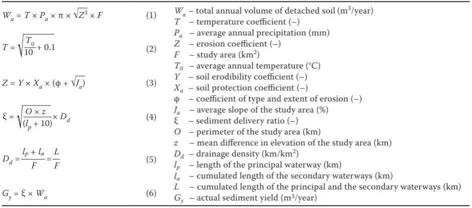
The Gavrilović method (Erosion Potential Meth-od, EPM) is an empirical, semi-quantitative model (Gavrilović 1972). The method was based on erosion field research in the Morava River catchment area in Serbia and encompasses erosion mapping, sediment quantity estimation, and torrent classification. Since 1968, the method has been extensively applied to erosion and torrent-related problems in the Balkan countries. It is currently being applied worldwide, from Switzerland, Croatia, Serbia, Slovenia, Italy, the Republic of Macedonia, Bosnia and Herzegovina, Montenegro, Iran to Chile (e.g. Bemporad et al. 1997; Globevnik et al. 2003; Fanetti & Vezzoi 2007; So-laimani et al. 2009; Amiri et al. 2012; Kayimierski et al. 2013; Spalević et al. 2013; Dragičević et al. 2014, etc.). The most often calculated outputs of the method (Table 1) are (i) the total annual volume of detached soil W_a (Table 1, Eq. (1)), (ii) the erosion coefficient Z (Table 1, Eq. (3)), and (iii) the actual sediment yield G_y (Table 1, Eq. (6)).

The Gavrilović method does not explore the phys-ics of erosion processes and as such it is advanta-geous for areas where minimal data are available or where there is a lack of previous erosion research. As such, the method provides an estimate not only of the amount of sediment production and sediment transport, but also of the resulting erosion intensity, Table 1. Equations and description of the parameters for the Gavrilović method (De Vente & Poesen 2005)

Wa = T × Pa×π × √Z3 × F (1) Wa – total annual volume of detached soil(m 3_/year)

T – temperature coefficient (–) Pa – average annual precipitation (mm)

Z – erosion coefficient (–) F – study area (km2₎

T0 – average annual temperature (°C)

Y – soil erodibility coefficient (–) X_a – soil protection coefficient (–)

φ – coefficient of type and extent of erosion (–) Ja – average slope of the study area (%)

ξ – sediment delivery ratio (–) O – perimeter of the study area (km)

z – mean difference in elevation of the study area (km) Dd – drainage density (km/km2)

lp – length of the principal waterway (km)

la – cumulated length of the secondary waterways (km)

L – cumulated length of the principal and the secondary waterways (km) Gy – actual sediment yield (m3/year)

(2)

Z = Y × X_a × (φ + √J_a) (3)

(4)

(5)

Gy = ξ × Wa (6)

T =

√

10

ξ =

√

Dd =

lp + la

and indicates areas of potential erosion threats. On the example of the Tartano Basin (Italy), Ballio et al. (2010) conducted sensitivity analysis of the Gavrilović method for only three parameters: (i) soil protection coefficient X_a, (ii) soil erodibility coefficient Y, and (iii) coefficient of type and extent of erosion φ with the parameter value deviation of –25% for X_a, +11% for Y, and +6.2% for φ in relation to values defined by the base case scenario. The authors noted the differ-ences between the obtained values for model outputs, ranging the values for the Actual sediment yield G_y from +5 to –35%, the former being the result of a change in parameter φ and the later in parameter X_a. Dragičević et al. (2014) analyzed uncertainties in the magnitude and spatial distribution of annual sediment production predictions in the Dubračina catchment, Croatia, where several alternative land cover/use inputs were applied. They used three different land cover/ use data sets: a CORINE land cover map, a Spatial Plan, and a Landsat 8 scene, and demonstrated the variations in the Gavrilović method output caused by different land cover/use inputs.

The analysis shown in this paper includes sensi-tivity analysis of all Gavrilović method parameters in relation to the following erosion model outputs: (i) the degree of annual soil loss (W_a), (ii) erosion intensity (Z), and (iii) eroded material transported through the river network (G_y). The analysis includes the calculation of the dimensionless Sensitivity In-dex I (Eq. (10)) (Lenhart et al. 2002) for each of the fourteen method parameters in relation to different model outputs. The dependence of model output y on any parameter x can be expressed as the partial derivative δ_y/δ_x. The approximation of this derivate is:

₍₇₎

where:

±Δx – variation in each parameter in relation to its value in the base model variant (Eqs (8) and (9)) y₁, y₂ – calculated model outputs for the defined

param-eter variation

x₁ = x₀ – Δx (8)

x₂ = x₀ + Δx (9)

Further, the calculated index Í must be normalized to obtain the sensitivity index I:

₍₁₀₎

The approach to sensitivity analysis and the deviation in parameters differ for different sensitivity methods and for different case studies. The differences in pa-rameters encompassed by sensitivity analysis can vary e.g. from 10% or more in parameter value and up to one- or several-times multiplied values of parameters Table 2. Sensitivity classes for Sensitivity index (Lenhart et al. 2002)

Class Index Sensitivity

I 0.00 ≤ |I| < 0.05 small to negligible II 0.05 ≤ |I| < 0.20 medium III 0.20 ≤ |I| < 1.00 high

IV |I| ≥ 1.00 very high

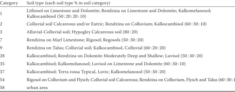
Table 3. Soil types of the Dubračina River catchment

Category Soil type (each soil type % in soil category)

1 _{Kalkocambisol (50 : 20 : 20 : 10)}Lithosol on Limestone and Dolomite; Rendzina on Limestone and Dolomite; Kalkomelanosol;

2 Colluvial soil Calcareous and/or Eutric; Rendzina on Colluvium; Kalkocambisol (60 : 30 : 10) 3 Alluvial-Colluvial soil; Hypogley Calcareous soil (80 : 20)

7 Rendzina on Marl Limestone; Rigosol; Regosols (50 : 30 : 20)

9 Rendzina on Talus; Colluvial soil; Kalkocambisol, Colluvial (60 : 20 : 20)

28 Kalkocambisol; Rendzina on Dolomite Moderately Deep and Shallow; Luvisol (50 : 30 : 20) 35 Kalkocambisol; Kalkomelanosol; Luvisol on Limestone and Dolomite (60 : 30 : 10) 37 Kalkocambisol; Terra rossa Typical, Luvic; Kalkomelanosol (50 : 30 : 20)

54 Rigosol on Colluvium and Flysch; Colluvial soil Calcareous; Rendzina on Colluvium, Flysch and Talus (60 : 30 : 10) 58 urban area

I' = y2 − y1 2Δx

I =

y2 − y1

y0

standard deviation (see Hamby 1994, 1995; Frey & Patil 2002; Cariboni et al. 2007; Satelli et al. 2008). The sensitivity index for each parameter, using the ap-proach proposed by Lenhart et al. (2002), is calculated such that only the parameter being evaluated is varied by ± 10% while all other parameters remain the same as in the base model variant. Each sensitivity index is then assigned a sensitivity class (Table 2) according to its resulting values for each individual parameter (Table 4) in relation to the output of the model.

The Gavrilović method sensitivity analysis is based on the example of the Dubračina River catchment area, Croatia (Figure 1). This small catchment (43 km2 in size) is characterized by its valuable natural and cultivated landscape, biodiversity, cultural and his-torical heritage as well as high annual rainfall, steep topography, and variable geology, all contributing to its land instability features such as landslides and excessive erosion processes. Although most of its tributaries (Figure 1a) tend to dry out dur-Figure 1. Dubračina catchment, Croatia: river network distribution and position of the town and meteorological station Crikvenica (a), elevation (b), soil type by category number (c), slope angle in degrees (d), land cover distribu-tion (e), and land cover in percentage (f)

Urban area 8% Water

1% Dense vegetation

(forest) 13%

Medium density vegetation

31% Bare soil to

rare vegetation

28% Bare rock

19%

Urban area 8% Water

1% Dense vegetation

(forest) 13%

Medium density vegetation

31% Bare soil to

rare vegetation

28% Bare rock

19%

Elevation (m a.s.l.)

Slope (°) Soil type

category

Land cover

(a) (b)

(c) (d)

(e)

(f)

0−50 50−100 100−200 200−300 300−400 400−500 500−600 600−700 700−800 800−920

ing the summer period, during the rainy period, considerable flow oscillations are very common. The overall catchment can roughly be divided into an upper karstic part with steep slopes and active sediment movement and a lower Flysch as a less permeable area. The complexity of soil structure in the Dubračina River catchment is evident from soil categories shown in Figure 1e and corresponding Table 3, where each category comprises several soil types whose interrelationship is defined by percentage ratio. The catchment stretches from 0 up to 920 m a.s.l. with steep slopes in its lower and upper part and less steep slopes in the middle part. The land cover description is based on Landsat 8 scene which recognizes six different land cover categories. Among them, medium density vegetation covers the largest area (31%) while bare soil to rare vegetation along with bare rock together covers 47% of the Dubračina catchment area. The complex geological structure, special valley cross section with distinct and steep slopes affected by erosion, local landslides and tor-rents, are the reason this area has been known for many years as an area of potential hazard.

For the purposes of this analysis, detailed and comprehensive data collection for the Dubračina catchment was conducted using sources from a variety of academic, governmental, and non-governmental institutions (Sušanj et al. 2013). The necessary data can be subdivided into spatially variant input parameters (land use/cover, precipitation, tempera-ture and land cover, soil erodibility, average slope of the study area, coefficient of type and extent of

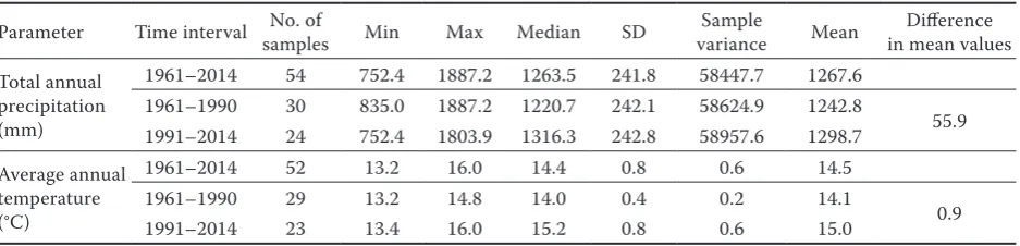
erosion, and mean difference in elevation of the study area) and spatially invariant parameters (study area, perimeter of the watershed, length of the principal waterways, and cumulated length of the principal and the secondary waterways). The spatial distributions of precipitation and temperature, with a resolution of 1000 × 1000 m, were obtained from the Croatian Meteorological and Hydrological Service for the time period of 1961–1990 (past time), as well as the average annual temperatures and the total annual pre-cipitation for the meteorological station Crikvenica (Figure 1a) from 1961 to 2014. Since all other data represent conditions on the catchment in the present time, the same had to be made for the precipitation and temperature with the assumption that the time period 1991–2020 represents the present time. Both the difference in the mean values between the two time periods (1961–1990 and 1991–2014) (Table 4) and trends encompassing the time range from 1961 to 2014 (Figure 2) indicate the increase in values for both parameters. The statistical analysis, t-test with 95% of confidence (two-tailed test), was conducted with a purpose to define if the difference within the mean values between the two time periods, for both temperature and precipitation, is significant. The null hypothesis assumes that the two data sets are likely to have come from distributions with equal popula-tion means. For the temperature parameter (P-value (9.21 × 10–8_{) < α (0.05)), the analysis has confirmed} a significant change in temperature mean values for the two time periods, which was not the case with the precipitation (P-value (0.249) > α (0.05)). Based

Figure 2. Average annual temperature and precipitation at the Crikvenica meteorological station from 1961 to 2014 and corresponding trends

y= 2.5905x– 3881 y= 0.0341x– 53.21

13 13.5 14 14.5 15 15.5 16 700 800 900 1000 1100 1200 1300 1400 1500 1600 1700 1800 1900 2000 19 61 19 63 19 65 19 67 19 69 19 71 19 73 19 75 19 77 19 79 19 81 19 83 19 85 19 87 19 89 19 91 19 93 19 95 19 97 19 99 20 01 20 03 20 05 20 07 20 09 20 11 20 13 To tal an nua l te m pe rature T0 (°C) A ve ra ge a nnu al p rec itip at io n Pa (mm ) Year

Total annual precipitation Average annual temperature

Lineární (Total annual precipitation) Lineární (Average annual temperature) y= 2.5905x– 3881 y= 0.0341x– 53.21

13 13.5 14 14.5 15 15.5 16 700 800 900 1000 1100 1200 1300 1400 1500 1600 1700 1800 1900 2000 19 61 19 63 19 65 19 67 19 69 19 71 19 73 19 75 19 77 19 79 19 81 19 83 19 85 19 87 19 89 19 91 19 93 19 95 19 97 19 99 20 01 20 03 20 05 20 07 20 09 20 11 20 13 To tal an nua l te m pe rature T0 (°C) A ve ra ge a nnu al p rec itip at io n Pa (mm ) Year

Total annual precipitation Average annual temperature

on twenty-four-year changes (data available from 1991 until 2014) in total annual rainfall and average annual temperature for the town of Crikvenica, and on the as-sumption that the spatial distribution pattern remains the same throughout the catchment for both past and present time series, the spatial distribution maps for these parameters were derived from the present time to correspond in all other input parameters.

Note that both the average annual temperature T₀ and the average annual precipitation P_a for the town of Crikvenica were found to increase in the period from 1991 till the present compared to the period 1961–1990 (by 0.9°C and 55.9 mm). The differences in the input data sets for temperature and precipita-tion are based on these changes.

The soil erodibility coefficient is based on a pedologi-cal map of Primorsko-Goranska County on a spedologi-cale of 1 : 100 000. The soil protection coefficient is based on the Landsat 8 data with a cell size 30 × 30 m. The land cover data that latter defines soil protection coefficient was obtained using supervised classification on the Landsat data and the ERDAS Imagine 2014 software. Furthermore, LIDAR data were used to generate a digital elevation model with a 2 × 2 m cell size spatial resolution, from which the average slope of the study area map and mean difference in elevation of the study area was derived. The coefficient of type and extent of erosion was based on the Spatial Plan map of known erosion-affected areas (scale 1 : 25 000). The drainage density map was based on river (primary and secondary) density calculated from the centre point of each map cell taking into account the values of all cells within the square of 1000 × 1000 m. The Map for the main difference in elevation of the watershed is produced in a similar way as the Drainage density map.

RESULTS

For the Gavrilović method sensitivity analysis, twenty-nine model variations were derived, and a

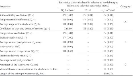
total of fourteen model parameters were analyzed and varied by ±10% to obtain the values for the Sensitiv-ity index I for each affected model output (Table 5). The included parameters can be divided into three categories: (A) the parameters that affect all three model outputs (W_a, G_y, and Z), (B) the parameters that affect both W_a and G_y, and (C) the parameters that only affect G_y.

The parameter with the highest sensitivity for all model outputs is the soil erodibility coefficient Y, fol-lowed by the soil protection coefficient X_a. Although overall X_a is a parameter with a very high sensitivity to the model, its slightly lower value compared to W_a classifies it as a high-sensitivity model parameter. All B category parameters are considered to be in the very high or high-sensitivity class in addition to the Average annual temperature T₀. It is well known that temperature and precipitation have a large impact on erosion processes, precipitation more than tempera-ture within the climate area for which the model was primarily developed. As expected, the model sensitivity class for the Average annual temperature T₀ is lower than the Average annual precipitation P_a but, when the Average annual temperature T₀ is transformed into its related form as the Temperature coefficient T, its sensitivity class is upgraded by one class.

The category C parameter with a very high sen-sitivity is the Sediment delivery ratio ξ, which is a product of all other category C parameters included in the analysis, all of which are in the high model sensitivity class except for the Length of the principal waterway l_p, with medium sensitivity.

DISCUSSION

Summarizing the analysis, the authors assigned sensitivity classes for each of the fourteen different parameters included in the method, with the objective of providing a better understanding of the method and the contributions of each parameter to differ-Table 4. Descriptive statistics for the precipitation and temperature parameters

Parameter Time interval No. of _samples Min Max Median SD _varianceSample Mean _{in mean values}Difference

Total annual precipitation (mm)

1961–2014 54 752.4 1887.2 1263.5 241.8 58447.7 1267.6 1961–1990 30 835.0 1887.2 1220.7 242.1 58624.9 1242.8

55.9 1991–2014 24 752.4 1803.9 1316.3 242.8 58957.6 1298.7

Average annual temperature (°C)

1961–2014 52 13.2 16.0 14.4 0.8 0.6 14.5

1961–1990 29 13.2 14.8 14.0 0.4 0.2 14.1

0.9

1991–2014 23 13.4 16.0 15.2 0.8 0.6 15.0

ent model outputs. The model outputs are mainly based on the multiplication of the model parameters; thus, for example, when varying the Average annual temperature P_a, the model outcome Total annual volume of detached soil W_a will vary proportion-ally. Not all parameters are included in the model through multiplication, e.g., Average slope of the study area J_a, Average annual temperature T₀, and Drainage density D_d Most of these parameters are categorized as high- or medium-sensitivity, whereas those in the multiplication form are classified as very high-sensitivity parameters.

It is for a discussion if the coefficient of type and extent of erosion φ should have lower impact upon the method outputs. Although sensitivity of the method output W_a in relation to φ is medium, its effect on Z and G_y remains classified as high. This parameter, although usefull, is one of the parameters that are not as commonly used as input parameter in other similar methods for erosion sediment assessment. The same can be said for O, z and l_p, l_a and L representatives of the study area characteristics, that highly affect G_y. Ballio et al. (2010) conducted the sensitivity analysis of the Gavrilović method for parameters φ, Y, X_a but left out a conclusion about the sensitivity parameter ranking. Nevertheless, they noted significant changes in model output values caused by the change in input

parameters, particularly soil protection coefficient X_a which is, according to sensitivity analysis conducted on the example of Dubračina catchment area, a high to very high-sensitivity parameter. Soil erodibility coefficient and soil protection coefficient X_a are considered very high-sensitive parameters with X_a being a high-sensitive parameter in relation to Wa model output. Dragičević et al. (2014) analyzed the effect of using different information sources for land use/cover parameter X_a and noted significant devia-tion in model output values. Although, their analysis explores the parameter uncertainty in a model, it is also closely related to parameter sensitivity analysis since both analyses take into consideration the de-viation in a parameter value, whether intentionally choosing the percentage for which its value will differ or choosing among various data whose deviation is defined by other external factors.

The second thing that should be taken into consid-eration during model calibration and modification in order to mitigate model errors and uncertainties is whether or not the average annual temperature is given a high enough significance in the model. The question is if the integration of T₀ in this way in the method restricts its use only within the areas of similar climate. Both precipitation and tempera-ture are considered to be highly significant by world

Table 5. Results of sensitivity analysis for Gavrilović model parameters in relation to model outputs

Parameter

Sensitivity class calculated in relation to model output

(calculated value for sensitivity index ) _Category W_a (m3_{/year) Z (–) G}

y (m3/year)

Soil erodibility coefficient(Y, –) IV (1.00) IV (1.01) IV (1.01)

A Soil protection coefficient (Xa, –) III (0.99) IV (1.00) IV (1.00)

Average slope of the study area (J_a, %) III (0.39) III (0.39) III (0.35) Coefficient of type and extent of erosion (φ, –) II (0.19) III (0.20) III (0.29)

Temperature coefficient (T, –) IV (1.01) – IV (1.01)

B

Erosion coefficient (Z, –) IV (1.00) – IV (1.00)

Average annual precipitation (Pa ,mm) III (0.99) – IV (1.00)

Study area (F, km2_{) III (0.99) – IV (1.00)}

Average annual temperature (T₀, o_{C) III (0.45) – III (0.46)}

Sediment delivery ratio (ξ, –) – – IV (2.23)

C

Drainage density (Dd, km/km2) – – III (0.99)

Perimeter of the study area (O, km) – – III (0.50)

Mean difference in elevation of the study area (z, km) – – III (0.50) Length of the principal waterway (lp, km) – – II (0.17) W_a – total annual volume of detached soil(m3_{/year); G}

scientific literature whereas within the Gavrilović method temperature is mitigated though the tem-perature coefficient.

Average slope length and gradient of the study area have a great impact upon water erosion, runoff, and downslope sediment transport and as such represent study area topography (Kinnell 2000; Blanco & Lal 2010; Shi et al. 2012). The impact of this parameter (J_a) upon a method outcome is high but according to its calculated values for sensitivity index I,J_a falls within parameters with lower high-sensitivity class values. All these parameters could potentially be used in future research where the need for its modification and method calibration presents for research areas with different characteristic (e.g. climate, geological, etc.) than those applied to this day.

Van Griensven et al. (2006) indicated the depend-ence of parameter sensitivity ranking, for higher ranked parameters, on the variable, the location, and case study. They highlighted the need for the sensitivity analysis to be conducted on each new catchment study in order to select a subset of pa-rameters to be used for model calibration or/and uncertainty analysis. Overall, the most sensitive model parameters resulting from the conducted sen-sitivity analysis for Gavrilović method are also those considered significant in the scientific literature on erosion (e.g. Toy et al. 2002; Morgan 2005, etc.).

Acknowledgements. The authors thank the University of Rijeka for financially supporting the publication of this paper (Research Project 13.05.1.3.08 – Development of New Methodologies in Water and Soil Management in Karstic, Sensitive and Protected Areas). This research was based on the work conducted within the following projects: Croatian-Japanese Project “Risk identification and Land-use Planning for Disaster Mitigation of Landslides and Floods in Croatia”, “Hydrology of Sensitive Water Resources in Karst” (114-0982709-2549) financed by the Ministry of Science, Education and Sports of the Republic of Croatia and Hydrology of water resources and risk identification of flooding and mudflows in the karst areas (13.05.1.1.03.).

References

Amiri F., Shariff A.R.B.M., Tabatabaie T. (2012): Monitor-ing land suitability for mixed livestock grazMonitor-ing usMonitor-ing Geographic Information System (GIS). In: Alam B.M. (ed.): Application of Geographic Information Systems. Rijeka, InTech: 241–266.

Ballio F., Brambilla D., Giorgetti E., Longoni L. (2010): Evaluation of sediment yield from valley slopes: a case study. In: de Wrachien D. (ed.): Monitoring, Simulation,

Prevention and Remediation of Dense and Debris Flows III. WIT Transactions on Engineering Sciences 67. South-ampton, WIT Press: 149–160.

Behnam N., Parehkar M. (2011): Sensitivity analysis of MPSIAC Model. Journal of Regeland Science, 1: 295–302. Bemporad G.A., Alterach J., Amighetti F.F., Peviani M.,

Saccardo I. (1997): A distributed approach for sediment yield evaluation in Alpine regions. Journal of Hydrology, 197: 370–392.

Blanco H., Lal R. (2010): Principles of Soil Conservation and Management. New York, Springer.

Cariboni J., Gatelli D., Liska R., Satelli A. (2007): The role of sensitivity analysis in ecological modelling. Ecological Modelling, 203: 167–182.

Chaves H.M.L., Nearing M.A. (1991): Uncertainty analysis of the WEPP soil erosion model. Transactions of the ASCE, 34: 2437–2444.

De Vente J., Poesen J. (2005): Predicting soil erosion and sediment yield at the basin scale: scale issues and semi-quantitative models. Earth-Science Reviews, 71: 95–125. De Roo A.P.J., Hazelhoff L., Burrough P.A. (1989): Soil

erosion modelling using ANSWERS and geographical information systems. Earth Surface Processes and Land-forms, 14: 517–532.

De Roo A.P.J., Hazelhoff L., Heuvelink G.B.M. (1992): Esti-mating the effects of spatial variability of infiltration on the output of a distributed runoff and soil erosion model using Monte Carlo methods. Hydrological Processes, 6: 127–143.

Dragičević N., Whyatt D., Davies G., Karleuša B., Ožanić N. (2014): Erosion model sensitivity to land cover inputs: case study of the Dubračina catchment, Croatia. In: Proc. 22nd _{Annual Conf. GISRUK 2014, Glasgow, Apr 16–18,}

2014: 340–348.

Fanetti D., Vezzoli L. (2007): Sediment input and evolu-tion of lacustrine deltas: the Breggia and Greggio rivers case study (lake Como, Italy). Quaternary International, 173–174:113–124.

Frey H.C., Patil S.R. (2002): Identification and review of sensitivity analysis methods. Risk Analysis, 22: 553–578. Gavrilović S. (1972): Engineering on torrential streams and

erosion. Izgradnja, Special Issue: 1–292. (in Serbian). Globevnik L., Holjevic D., Petkovsek G., Rubinic J. (2003):

Applicability of the Gavrilovic method in erosion calcula-tion using spatial data manipulacalcula-tion techniques, erosion prediction in Ungauged Basins: integrating methods and techniques. In: Proc. Int. Symp. HS01, Erosion Predic-tion in Ungauged Basins (PUBs): Integrating Methods and Techniques, Sapporo, July 8–9, 2003, IAHS Publ. No. 279: 224–233.

Hamby D.M. (1995): A comparison of sensitivity analysis techniques. Health Physics, 68: 195–204.

Jetten V., de Roo A., Favis-Mortlock D. (1999): Evaluation of field-scale and catchment-scale soil erosion models. Catena, 37: 521–541.

Jetten V., Gouvers G., Hessel R. (2003): Erosion models: quality of spatial predictions. Hydrological Processes, 17: 887–900.

Kayimierski L.D., Irigoyen M., Re M., Menendey A.N., Spalletti P., Brea J.D. (2013): Impact of climate change on sediment yield from the upper Plata basin. International Journal of River Basin Management, 11: 1–11.

Kinnell P.I.A (2000): The effect of slope length on sediment concentrations associated with side-slope erosion. Soil Science Society of America Journal, 64: 1004–1008. Lane J.W., Ferriera V.A. (1982): Sensitivity analysis. In:

Kin-sel W.G. (ed.): CREAM, A Field Scale Model for Chemi-cal, Runoff and Erosion from Agricultural Management Systems A. Model Documentation. USDA Conservation Research Report No. 26. Washington, USDA: 113–158. Lenhart T., Eckhardt K., Fohrer N., Frede H.-G. (2002):

Comparison of two different approaches of sensitivity analysis. Physics and Chemistry of the Earth, 27: 645–654. Liu L., Liu X.H. (2010): Sensitivity analysis of soil erosion in the Northern Loess Plateau. Procedia Environmental Sciences, 2: 134–148.

Loucks D.P., van Beek E. (2005): Water Resources Sys-tems Planning and Management – An Introduction to Methods, Models and Applications. Paris, UNESCO Publishing.

Mendicino G. (1999): Sensitivity analysis on GIS procedures for the estimate of soil erosion risk. Natural Hazards, 20: 231–253.

Merritt W.S., Letcher R.A., Jakeman A.J. (2003): A review of erosion and sediment transport models. Environmental Modelling and Software, 18: 761–799.

Misra R.K., Rose C.W. (1996): Application and sensitivity analysis of process-based erosion model GUEST. Euro-pean Journal of Soil Science, 47: 593–604.

Morgan R.P.C. (2005): Soil Erosion & Conservation. Oxford, Blackwell.

Nearing M.A., Deer-Ascough L., Laflen J.M. (1990): Sen-sitivity analysis of the WEPP hillslope profile erosion model. Transactions of the ASAE, 33: 839–849.

Nord G., Esteves M. (2005): PSEM_2D: A physically based model of erosion processes at the plot scale. Water Re-sources Research, 41(W08407): 1–14.

Satelli A., Ratto M., Andres T., Campolongo F., Cariboni J., Gateli D., Saisana M., Tarantola S. (2008): Global Sensitiv-ity Analysis: The Primer. Willey, Chichester.

Shi Z.H., Fang N.F., Wu F.Z., Wang L., Yue B.J., Wu G.L. (2012): Soil erosion processes and sediment sorting as-sociated with transport mechanisms on steep slopes. Journal of Hydrology, 454–455: 123–130.

Solaimani K., Modallaldoust S., Lotfi S. (2009): Soil ero-sion prediction based on land use changes (A case in Neka wathershed). American Journal of Agricultural and Biological Sciences, 4: 97–104.

Spalevic V., Djurovic N., Mijovic S., Vukelic-Sutoska M., Curovic M. (2013): Soil erosion intensity and runoff on the Djuricka River Basin (north of Montenegro). Malay-sian Journal of Soil Science, 17: 49–68.

Sušanj I., Dragičević N., Karleuša B., Ožanić N. (2013): GIS based monitoring database for Dubračina river catchment area as a tool for mitigation and prevention of flash flood and erosion. In: Proc. 13th _{Int. Symp. Water Management and}

Hydraulic Engineering, Bratislava, Sept 9–12, 2013: 637–652. Tattari S., Bärlund I. (2001): The concept of sensitivity in

sediment yield modelling. Physics and Chemistry of the Earth, 26: 27–31.

Toy T.J., Foster G.R., Renard K.G. (2002): Soil Erosion: Processes, Prediction, Measurement, and Control. New York, John Wiley & Sons.

Tucker G.E. (2004): Drainage basin sensitivity to tectonic and climatic forcing: implications of a stochastic model for the role of entrainment and erosion thresholds. Earth Surface Processes and Landforms, 29: 185–205. Tucker G.E., Whipple K.X. (2002): Topographic outcomes

predicted by stream erosion models: Sensitivity analysis and intermodal comparison. Journal of Geophysical Re-search: Solid Earth, 107(B9): 1–16.

van Griensven A., Meixner T., Grunwald S., Bishop T., Diluzio M., Srinivasan R. (2006): A global sensitivity analysis tool for the parameters of multi-variable catch-ment models. Journal of Hydrology, 324: 10–23. Veihe A., Quinton J. (2000): Sensitivity analysis of EUROSEM

using Monte Carlo simulation I: hydrological, soil and veg-etation parameters. Hydrological Processes, 14: 915–926. White K.L., Chaubey I. (2005): Sensitivity analysis, calibra-tion, and validations for a multisite and multivariable SWAT model. Journal of the American Water Resources Association, 41: 1077–1089.