On the choice of covariance specifications for portfolio selection problems

(1)

Munich Personal RePEc Archive

On the choice of covariance specifications

for portfolio selection problems

R. Ferreira, Alexandre and A. P. Santos, Andre

21 August 2016

Online at

https://mpra.ub.uni-muenchen.de/73259/

(2)

On the choice of covariance specifications for portfolio selection

problems

Alexandre R. Ferreira

∗1

and Andr´

e A. P. Santos

2

1

_{PhD Candidate in Business, Rice University}

2

_{Department of Economics, Universidade Federal de Santa Catarina}

August 21, 2016

Abstract

Two crucial aspects to the problem of portfolio selection are the specification of the model for expected returns and their covariances, as well as the choice of the investment policy to be adopted. A common trade-off is to consider dynamic covariance specifications vis-a-vis static models such as those based on shrinkage methods. This work empirically shows that these two aspects are intrinsically attached to the impact of transaction costs. To address this question, we implement a broad range of covariance specifica-tions to generate a set of 16 portfolio selection policies in a high dimensional sample composed by the 50 most traded stocks of the S&P100 index. We find that GARCH-type dynamic covariances yield portfolios with superior risk-adjusted performance only in the absence of transaction costs. In more realistic scenarios involving alternative levels of transaction costs, portfolios based on static covariance models outperform. In particular, we find that a risk-averse investor with quadratic utility function is willing to pay an annualized fee of 368 basis points (bp) on average in order to switch from the dynamic covariance models to a static covariance specification when the level of transaction costs is 20 bp. Finally, portfolio policies that seek to alleviate estimation error by ignoring off-diagonal covariance elements as those proposed in Kirby & Ostdiek (2012) are more robust specially in scenarios with higher transaction costs.

(3)

1 Introduction

This paper is concerned with the problem of the choosing the most appropriate covariance specification for high

dimensional portfolio selection and optimization. This choice is of paramount importance since the specification

of the covariance matrix of asset returns is a key ingredient to many portfolio selection problems. Markowitz

(1952), for instance, created the basis for the modern portfolio theory by showing the way in which variances

and covariances influence portfolio risk and risk-adjusted portfolio returns. Since then, academics and market

practitioners seek to enhance covariance modeling using a myriad of methods and models.

The literature points to an ample range of possible ways of modeling covariances. The most immediate choice

is usually between static or dynamic models. Dynamic models are based on the idea that the current covariance

depends on the covariance of previous periods, being updated according to alternative autoregressive structures

such as multivariate GARCH and stochastic volatility models; see Bauwens et al. (2006) and Silvennoinen & Ter¨asvirta (2009). Static models, in constrast, are those in which which there is no autoregressive covariance

dynamics and, because of that, are usually more parsimonious than their dynamic counterparts. The most

common static models are those in which the covariance matrix is unconditionally estimated using on a sample

of asset returns or, alternatively, estimated based on a factor model that captures cross-sectional characteristics

of asset returns. Among static models commonly employed in portfolio selection problems are the ones that

reduce estimation error by shrinking the sample covariance matrix towards alternative targets such as those

proposed in Ledoit & Wolf (2003a,b, 2004).

To ground the decision of which type of covariance model to adopt, usually are taken into account pros and

cons of each approach as, for example, ease of implementation, processing cost, as well as the ability to capture

stylized facts in the covariance profile among the assets. One central aspect that must be taken into account

while choosing the most appropriate covariance specification is that dynamic models usually posses the highest

implementation requirements when compared to their static counterparts due to their increased

parameteriza-tion. This leads to more estimation error and negatively impact portfolio performance, due to demanding more

frequent portfolio re-balancing and yielding more extreme portfolio allocations, and, consequently, increasing

transaction costs (Kirby & Ostdiek, 2012). On the other hand, these models can accommodate stylized facts of

financial time series such as hetoskedasticity and excess kurtosis.

In this paper we shed light on the lack of consensus in the literature regarding which is the most appropriate

approach to model covariances in a realistic scenario in which i) there are many assets, ii) transaction costs

are properly taken into account, and iii) there is frequent portfolio re-balancing. Our main goal is to evaluate

i) how the increase in proportional transaction costs impacts portfolio performance measured by risk-adjusted

returns net of transaction costs and ii) how this information can be used in order to help investors to select the

most appropriate covariance specification.

Our paper is related to previous studies in the literature of covariance modeling for portfolio selection

(4)

the performance of alternative dynamic covariance specifications belonging to the multivariate GARCH family

and conclude that tightly parameterized models generally perform better when evaluated with economically

meaningful criteria. Beckeret al. (2014) study the ability of different loss functions to discriminate between a set of competing forecasting models which are subsequently applied in a portfolio allocation context. None of

the studies, however, consider the impact of transaction costs and employ only one portfolio selection policy.

We add to this literature by not only taking into account the presence of transaction costs but also considering

a broader set of portfolio policies.

It is also worth mentioning that the estimation of expected returns also plays its part in portfolio

selec-tion. There is evidence, however, suggesting that employing predictive models for expected returns based on

autoregressive structures leads to portfolios with very high turnovers that might compromise their usage in real

situations; see, for example, DeMiguelet al. (2009a) and DeMiguelet al. (2014). Because of that, the present work considers less parameterized alternatives. Specifically, we i) estimate expected returns either

uncondition-ally via sample means or ii) assumes that a multi-factor conditional version of the capital asset pricing model

(CAPM) holds, which implies that the cross-sectional variation in conditional expected excess returns is due to

cross-sectional variation in conditional betas.

In our empirical exercise we implement 11 different covariance models to generate a set of 16 portfolios

from different asset selection strategies in a high dimensional sample composed by the 50 most traded stocks

from the S&P100 index. We choose 3 popular static models based on shrinkage methods proposed in Ledoit

& Wolf (2004), Ledoit & Wolf (2003a) and Ledoit & Wolf (2003b). In short, these models shrink the sample

covariance matrix, which is an unbiased estimator but more prone to estimation error, towards alternative

structured covariance estimators that are biased but less prone to estimation error. In this case, the target

matrices are the identity matrix, constant correlation matrix and market factors matrix, respectively. The

remaining 8 specifications belong to the class of dynamic covariance models models from the multivariate

GARCH family: the exponentially weighted moving average (EWMA), the optimal rolling estimator (ORE)

of Foster & Nelson (1996), the scalar VECH model of Bollerslev et al. (1988), the orthogonal GARCH (O-GARCH) from Alexander (2001), the constant conditional correlation (CCC) model of Bollerslev (1990), the

dynamic conditional correlation model (DCC) proposed by Engle (2002), and its asymmetric version (ASYDCC)

proposed in Cappielloet al. (2006). Each of these specifications are detailed in Section 3.

The alternative covariance specifications are used to obtain a set of portfolio policies including alternative

formulations of the mean-variance policy such as those that alleviate estimation risk by imposing short-sales

restrictions (Jagannathan & Ma, 2003) and norm restrictions (DeMiguel et al. , 2014). We also implement a second group of portfolio policies that aims at reducing estimation risk by ignoring off-diagonal covariance

elements such as those proposed in Kirby & Ostdiek (2012). These policies retain the most appealing features

(5)

the assets under consideration.

Our results leave three most important messages. First, the choice of the covariance model is critical to

the performance of a portfolio policy. For instance, we find the risk-adjusted performance measured by the

Sharpe ratio can vary from -0.62 to 0.06 within the same portfolio policy by changing the covariance model used

to obtain portfolio weights. Second, we find that the choice of the most appropriate covariance specification

for the portfolio selection problems considered in the paper is substantially impacted by the presence and

the level of transaction costs. We find that, in the absence of transaction costs, dynamic covariance models

outperform static counterpars in terms of average gross returns as well as in terms of risk-adjusted returns.

On average, Sharpe ratios obtained with dynamic covariance models are 12% higher than those obtained with

static covariance models, and the pairwise differences are statistically significant in many instances. However,

as we move to more realistic scenarios in which transaction costs are properly taken into account, we find that

static covariance models clearly outperform in the vast majority of instances. Specifically, Sharpe ratios based

on portfolio returns net of transaction costs of 20 basis points (bp) are 48% higher on average when static

covariance models are adopted in comparison to those obtained with dynamic models. This difference in risk

adjusted performance becomes even higher when transaction costs of 50 bp are considered. A closer examination

reveals that these differences in risk-adjusted performance are mainly driven by a much higher level of turnover

obtained when dynamic covariance models are used to implement the portfolio policies. Finally, we find that

a risk-averse investor with quadratic utility function is willing to pay an annualized fee of 368 bp on average

in order to switch from the dynamic covariance models to a static covariance specification when the level of

transaction costs is 20 bp.

The remainder of the document is organized this way: section 2 details the portfolio selection policies

considered in the paper. Section 3 describes the dynamic and static covariance models. Section 4 discusses

the methodology used to evaluate portfolio performance. Section 5 details the empirical exercise carried out.

Finally, Section 6 concludes.

2 Portfolio selection methods

Consider an investment universe withN assetsA1, A2, . . . , AN with uncertain future returnsR1, R2, . . . , RN.

LetRbe the return vector:

R= [R1, R2, . . . , Rn]⊺.

The expected return vectorµ=E(R) contains as its elementsµi=E(Ri),i= 1, . . . , n, such that:

(6)

The covariance matrix of the returns, Σ =V ar(R), contains as its elements σii =σi2 andσij =σji =ρijσiσj

(fori 6=j), where σi is Ri standard deviation andρij is the correlation between the returns of assetsAi and

Aj (fori6=j). The covariance matrix Σ is symmetric and written as:

Σ = (σij)_i,j₌₁_,...,N =

        

σ11 σ12 · · · σ1n

σ21 σ22 · · · σ2n

..

. ... . .. ...

σn1 σn2 · · · σnn

        

.

All valid covariance matrices are positive semi-definite, or equivalently, all eigenvalues are non-negative. A

portfolio is represented by theN-dimensional vectorw, such that:

w= [w1, w2, . . . , wn]⊺,

andwi is the share of total wealth invested in assetAi. The portfolio return Rp is linearly dependent of these

weights and it is the weighted average of the returns of each asset involved, where the weight of each asset is

the portfolio share invested in the asset, i.e.:

Rp=w1R1+· · ·+wnRn= N

X

i=1

wiRi=w⊺R.

Therefore, the expected portfolio return, µp, is the weighted average of each asset expected return and the

portfolio varianceσ2

p is a quadratic function of the weight vector. We can denote these variables by:

µp=E(Rp) =E(w⊺R) =w⊺µ (1)

σ2p=V ar(Rp) =V ar(w⊺R) =w⊺Σw. (2)

2.1 Policies

Assume that there areN risky assets with expected returns µtand covariance matrix Σt. Suppose that there

is no risk free asset and that the investor need to allocate all his wealth among the N risky assets. Next, we

detail the portfolio selection policies considered in our empirical exercise.

(7)

between risk and return the investor needs to find the weight vector that satisfies:

min

wt

w⊺

tΣtwt−

1

γw

⊺

tµt,

s.t.w⊺

te= 1 (3)

whereγ >0 represents the investor’s level of relative risk aversion andeis a vector of ones. µt= _T1 T

P

i=1

R

is the vector of expected returns, whereT is the length of the estimation window. The specification of the

covariance matrix Σt depends on whether we are using a dynamic or a static model; see Section 3. The

component w⊺

tΣtwt represents the portfolio risk. The component w⊺tµt represents the portfolio return.

We follow DeMiguel et al. (2009a) and set γ = 1.1 _{We refer to this formulation as the unrestricted}

mean-variance (MeVU) portfolio.

When considering the case where the investor risk aversion tends to the infinity (γ → ∞) the problem

can be represented as

min

wt

w⊺

tΣtwt,

s.t.w⊺

te= 1. (4)

In this case, the investor only cares about reducing the portfolio risk, without considering the expected

return. This is an important portfolio policy since expected returns is subjected to more estimation

errors when compared to the estimation of covariances (Merton, 1980). We refer to it as the unrestricted

minimum variance portfolio (MiVU).

One popular variation of the traditional mean-variance formation is to include a constraint on short-sales.

Jagannathan & Ma (2003) show that including this restriction alleviates estimation error in portfolio

weights. The constrained-version formulation for the mean-variance problem can be specified as

min

wt

w⊺

tΣtwt−1

γw

⊺

tµt,

s.t.w⊺

te= 1 (5)

wt≥0

where the restriction wt ≥0 represents the short-sale restriction. We refer to it as the restricted

mean-1

(8)

variance (MeVC) portfolio . Similarly, the restricted minimum variance (MiVC) portfolio is given by:

min

wt

w⊺

tΣtwt,

s.t.w⊺

te= 1 (6)

wt≥0.

Norm-constrained mean-variance. We follow DeMiguelet al. (2014) and consider a class of mean-variance portfolios with norm restriction (NCMV) given by:

min

wt

w⊺

tΣtwt−

1

γw

⊺

tµt,

s.t.w⊺

te= 1 (7)

kwt−w0tk1=

N

X

i=1

|(wt)i−(w0t)i| ≤δ

wherew0tis the vector of weights of the MeVC portfolio andδis the maximum deviation from the norm.

The norm restriction requires that the weights of this portfolio remain close to the weights of the MeVC

portfolio, as the aggregate absolute distance between the weights cannot be greater than the norm. We

follow DeMiguelet al. (2014) and use the 1-norm in relation to the restricted mean-variance. Moreover, we consider the maximum deviation to the norm, δ, to be equal to 2.5%, 5.0% and 10.0%. We refer to

these portfolios as NCMV2.5, NCMV5, and NCMV10, respectively.

Volatility timing and reward-to-risk. We implement the volatility timing (VT) portfolio policy proposed in Kirby & Ostdiek (2012). These policies greatly simplify the computation of optimal weights by setting

off-diagonal covariance elements equal to 0 and therefore reducing estimation error. The VT policy assumes

that portfolio weight in theith_{asset is inversely proportional to its estimated variance, i.e.,}

ˆ

wit=

1 ˆ

σ2

it

η

N

P

i=1

1 ˆ

σ2

it

η (8)

where ˆσitis the volatility of theithasset. The parameter ηmeasures the aggressiveness of the allocation.

The tuning parameterη ≥0 determines how aggressively we adjust the portfolio weights in response to

changes in the assets’ variances. As η→0 we recover the equally-weighted portfolios, and asη→ ∞the

weight on the asset with lowest variance approaches 1. Thus, large values of η, can shrink the portfolio

weights towards the less risky assets. We follow Kirby & Ostdiek (2012) and considered η equals to 1, 2

and 4 thus yielding the VT1, VT2, and VT4 policies, respectively.

(9)

information about conditional expected returns, and therefore selecting assets according to their

risk-return trade-off. The reward-to-risk (RwR) policy is defined as

ˆ

wit=

_µ_ˆ+

it ˆ σ2 it η N P i=1

_µ_ˆ+

it

ˆ

σ2

it

η (9)

where ˆµ+_it= max(ˆµit,0) and ˆµitis theithasset expected return i.e. µit=_T1 T

P

i=1

Ri whereT is the length of

the estimation window. We follow Kirby & Ostdiek (2012) and implement the RwR polcy by considered

η equals to 1, 2 and 4 thus yielding the RwR1, RwR2, and RwR4 policies, respectively.

Finally, we also consider a variation of the RwR policy that aims at improving the estimation of expected

returns by considering a factor model. One immediate choice is to assume that that a conditional version

of the capital asset pricing. The conditional CAPM implies that the cross-sectional variation in conditional

expected excess returns is due to cross-sectional variation in conditional betas. This approach, however,

can also be extended to multiple risk factors. The resulting weights for the RwR strategy is

ˆ

wit=

_β¯+

it ˆ σ2 it η N P i=1

β¯+

it

ˆ

σ2

it

η (10)

where ¯β+_it = max( ¯βit,0) and ¯βit= (1/K) K

P

j=1

βij,t is the average conditional beta of assetiwith respect to

the K factors. To implement this policy, we consider the 4-factor model proposed by Carhart (1997) as

an extension to the 3-factor model proposed by Fama & French (1992). Similar as in the VT policies, we

consideredηequals to 1, 2 and 4 thus yielding the RwR4F1, RwR4F2, and RwR4F4 policies, respectively.

3 Covariance models

In this Section we describe the alternative approaches we use to model covariances in our empirical exercise.

We initially describe the static models based of the shrinkage methods proposed in Ledoit & Wolf (2003a,b,

2004). Later, we describe the dynamic specifications based on the multivariate GARCH family.

3.1 Shrinkage methods

The shrinkage method used to model covariances is based on the bias-variance trade-off. The method considers

that a way to obtain a better covariance estimator is to simply take a weighted average between a biased

estimator, with little estimation error, and an unbiased one, but with a lot of estimation error. This process

(10)

This idea can be summarized as

Σt= ˆδFt+ (1−ˆδ)St, (11)

where 0≤δˆ≤1 is the estimated shrinkage intensity,F is usually a highly structured covariance matrix, andS

is an unstructured estimator. The sample covariance matrix estimated as ˆSt= (1/T)PTt=1(Rt−µˆt) (Rt−µˆt)

′

is most frequently used as this unstructured estimator. The structured estimator usually reflects important

characteristics of the variable being estimated. We considered as target covariances those considered in Ledoit

& Wolf (2003a,b, 2004).

Ledoit & Wolf (2003a) uses a model of constant correlation between the assets in order to define the target

structured estimator F. To define this covariance matrix, let St be the sample covariance and sij,t be the

element of St at row i and column j. So the sample correlation is defined as rij,t = sij,t/√sii,tsjj,t, whose

average is ¯rt=₍_N−21)N N_P−1

i=1

N

P

j=i+1

rij,t. Therefore, the constant correlation matrixFtcan be obtained using the

sample variances and the sample average correlation, i.e. fii,t=sii,tandfij,t= ¯rt√sii,tsjj,t, wherefij,t be the

element ofFtat rowiand column j.

Ledoit & Wolf (2003b) assume an one factor market model for the return of asset j at timet:

rj,t=αj+βjrM,t+ǫj,t,

whererM,tis the market index return at timet,βj is the load on the market factor,αj is the intercept andǫj,t

is the error. Assuming thatrM,tand ǫj,t are uncorrelated and thatǫi,t andǫj,t are uncorrelated fori6=j, the

structured target covariance matrix is defined as

Ft=sm,tBB⊺+Dt, (12)

whereB is the vector ofβs,sm,tis the sample variance ofrM,tandDtin the diagonal matrix consisting of the

variance of the sample errors. Finally, Ledoit & Wolf (2004) use the identity matrix as the target structured

estimator, i.e. Ft=I.

One appealing aspect of the three shrinkage methods described above is that the computation of the shrinkage

intensity ˆδ is based on closed form expressions. A description of these expressions can be found in Ledoit &

Wolf (2003a,b, 2004).

3.2 Multivariate GARCH models

The conditional covariance models considered in this paper belong to the class of multivariate GARCH models.

For that purpose, we assume that the multivariate system of asset returns is conditionally heteroskedastic and

followsRt=zt(Σt)1/2. To model Σt, we implement 8 specifications commonly used in portfolio selection

(11)

each of the conditional covariance specification employed in the paper.

Exponentially weighted moving average (EWMA): The EWMA model is defined as

Σt=αRt−1

′

Rt−1+ (1−α) Σt−1,

where αis a non-negative parameter. When theαis set to a fixed value of 0.04, the EWMA is equivalent to

the popular Riskmetrics approach. Zaffaroni (2008) shows that although it permits sizable computational gains

and provide a simple way to impose positive semi-definiteness of the resulting conditional covariance matrices,

the Riskmetrics delivers non-consistent estimates. Therefore, in our implementation of the EWMA specification

the parameterαis estimated via maximum likelihood; see details below.

Optimal rolling estimator (ORE): The general rolling estimator is defined as Σt=

∞

P

k=1

Ωt−k⊙Rt−k

′ Rt−k,

where Ωt−k is a symmetric matrix of weights and ⊙ denotes the element-by-element multiplication. This

structure admits a wide range of potential weighting schemes. Foster & Nelson (1996) show that the optimal

strategy is to let the weights decline in an exponential fashion as the magnitude ofkincreases. Their procedure,

however, implies a different decay rate for each element of the conditional covariance matrix Σt. Because this

makes it difficult to ensure that the resulting matrix is positive definite, we follow Fleminget al. (2001, 2003) and impose the restriction Ωij,t = Ωt for all i and j. In this case, the optimal weighting scheme is given by

Ωt−k=αexp (−αk)ι′ι whereαis the decay rate andιis a vector of ones. Therefore, the rolling estimator can

be rewritten as

Σt=αexp (−α)Rt−1

′

Rt−1+ exp (−α)Ht−1, (13)

where αis a nonnegative parameter which is estimated via maximum likelihood; see details below. In (13) a

single parameter (α) controls the rate at which the weights decay with the lag length. This parsimony facilitates

estimation specially when the dimension is high. The ORE specification has been applied in many portfolio

selection problems such as in Fleminget al. (2001, 2003) and Pooter et al. (2008). Fleminget al. (2003), in particular, point out that covariance matrix forecasts based on the ORE specification results in better portfolios

in comparison to those obtained with other (unrestricted) multivariate GARCH models. The authors argue

that the smoothness of the rolling estimator as the main reason for this.

Scalar VECH: The scalar VECH specification of Bollerslevet al. (1988) is defined as

Σt=C′C+αRt−1Rt−1

′

+βHt−1.

(12)

in Engle & Mezrich (1996). The general idea is to estimate the intercept matrix by an auxiliary estimator that

is given by ˆC′ˆ

C = ¯S(1−α−β), where ¯S = _T1

T

P

t=1

RtRt′, thus yielding the variance-targeting scalar VECH

model

Σt= ¯S(1−α−β) +αRt−1Rt−1

′

+βHt−1, (14)

which is covariance-stationary provided thatα+β <1.

Orthogonal GARCH (O-GARCH): The O-GARCH model of Alexander (2001) belongs to a class of factor models and is able to achieve significant computational gains via dimensionality reduction. The O-GARCH

model is given by Σt=WΩtW, whereW is aN×kmatrix whose columns are given by the firstkeigenvectors

of thet×N matrix of asset returns, and Ωtis ak×kdiagonal matrix whose elements are given byhfkt where

hfkt is the conditional variance of thek-th principal component and follows a GARCH(1,1) process. We follow

Engle & Sheppard (2008) and implement the O-GARCH model using 3 principal components.

Conditional correlation models: This class of models is defined as Ht =DtΨtDt, whereDt is a N ×N

diagonal matrix with diagonal elements given by hi,t, where hi,t is the conditional variance of the i-th asset

and follows a GARCH(1,1) process, and Ψt is a symmetric conditional correlation matrix with elementsρij,t,

where ρii,t= 1, i, j = 1, . . . , N. We consider 4 alternative specifications to model Ψt: (i) the constant

condi-tional correlation (CCC) model of Bollerslev (1990), (ii) the dynamic condicondi-tional correlation (DCC) model of

Engle (2002), (iii) the asymmetric DCC (ASYDCC) of Cappielloet al. (2006), (iv) the dynamic equicorrelation (DECO) model of Engle & Kelly (2012). Engle & Colacito (2006) and Engle & Sheppard (2008) study the

performance of alternative conditional correlation models in portfolio selection problems.

Multivariate GARCH models are typically estimated via quasi maximum likelihood (QML). However, this

estimator is found to be severely biased in large dimensions; see, for instance, Engleet al. (2008) and Hafner & Reznikova (2012). In this paper, the parameters of the EWMA, ORE, and VECH specifications are estimated

with the composite likelihood (CL) method proposed by Engleet al. (2008). As for the conditional correlation models, their estimation can be conveniently divided into volatility part and correlation part. The volatility part

refers to estimating the univariate conditional variances which is done by QML assuming Gaussian innovations.

The parameters of the correlation matrix in the DCC and ASYDCC models are estimated using the CL method.

(13)

4 Methodology for evaluating portfolio performance

To implement the portfolio policies described in Section 2 alongside the covariance models discussed in Section

3, we adopt a recursive estimation approach that works as follows. First, we use an initial estimation window

ofT = 1500 daily observations to estimate all covariance models (11 models). As for the dynamic ones, we also

obtain one-step-ahead forecasts of the conditional covariance matrix for the period 1501. Second, we implement

each of the portfolio policies (16 in total) using each of the estimated covariances, therefore yielding a total

of 16×11 = 176 different portfolios. Third, we compute portfolio statistics for each for period 1501 using

the methodology described in Section 4. Fourth, we add one observation to the estimation window and repeat

this process until the end of the data set is reached. We end up with a sample ofL−T pseudo out-of-sample

observations, whereL is the length of the data set, which are used to evaluate the performance of each of the

176 portfolios. Portfolos are re-balanced on a daily basis.

Holding the portfolio wtfor one day gives the out-of-sample portfolio return at timet+ 1: Rp,t =w′tRt+1

whereRt+1is the vector of asset returns. We use the time series of out-of-sample portfolio returns and weights

of each portfolio policy described in Section 2 to evaluate the performance in terms of average return (ˆµ) and

standard deviation (volatility) of returns (bσ). These statistics are calculated as follows:

ˆ

µ= 1

T−1

T_X−1

t=1

w′

tRt+1

ˆ

σ=

v u u t 1

T−1

T_X−1

t=1

(w′

tRt+1−Rp)2.

whereRpis the realized portfolio average return.

A crucial aspect that must be taken into account is the impact of transaction costs on the performance of

optimal portfolios (Han, 2006). As Kolm et al. (2014) points out, transaction costs consist of direct costs, such as commissions and taxes, bid-ask spread, and indirect costs, such as slippage. As in Olivares-Nadal &

DeMiguel (2015), for small trades, which do not impact the market price, the transaction cost is assumed to

proportional to the amount traded on each asset. To take into account the impact of proportional transaction

costs, we follow Della Corteet al. (2008) and Thornton & Valente (2012) and compute the portfolio return net of transaction costs (Rnet

p,t). This calculation is performed as

Rnetp,t = (1−c·turnovert) (1 +wt′Rt+1)−1, (15)

where c is the fee that must be paid for each transaction and turnovert is the portfolio turnover at time t,

defined as the fraction of wealth traded between periodstand t+ 1, i.e

turnovert= N

X

j=1

(14)

To compute (15), it is necessary to set an appropriate value for the transaction costc. French (2008) estimates

how much Americans spend on transaction costs each year for different active investing options, and compare

it with the cost of passive investing. He finds that Americans spend 21 basis points (bp) in total trading, as a

fraction of the total portfolio. Therefore, in order to evaluate the impact of transaction costs on the performance

of the alternative portfolio selection policies, we follow Kirby & Ostdiek (2012) and consider three alternative

scenarios of transaction costs: 0 bp (no transaction costs), 20 bp (intermediate level of transaction costs), and

50 bp (high level of transaction costs).2

Upon computing the average and the standard deviation of the portfolio return net of transaction costs for

based on each of the three levels of transaction costs considered in the paper, we compute the average portfolio

turnover over all observations as well as the risk-adjusted portfolio return net of transaction costs measured by

the Sharpe ratio (SR), which is defined as

SR=R¯p

net

σnet , (16)

where ¯Rp

net

and σnet _{are, respectively, the average and the standard deviation of portfolio returns net of}

transaction costs.

In order to assess the relative performance of portfolios obtained with dynamic covariance models with respect

to those obtained with static models, we implement the bootstrap test for the differences in SR proposed by

Ledoit & Wolf (2008). For that purpose, we select as main benchmark the portfolios obtained with the shrinkage

method proposed in Ledoit & Wolf (2004). In other words, we test for the differences in Sharpe ratios obtained

with a dynamic covariance model with respect to those obtained with a static model within the same portfolio

selection policy.

Finally, we also follow Fleminget al. (2001) and Kirby & Ostdiek (2012) and use a utility-based approach to measure the value of the performance gains associated with employing a given portfolio strategy along with

a specific choice for the covariance model. We assume the investor has a quadratic utility function given by:

U(Rp,t) =W0

1 +Rp,t−

γ

2 (1 +γ)(1 +Rp,t)

2

,

whereRp,t=wt′−1Rtis the portfolio return,γis the investor’s relative risk aversion andW0is the initial wealth.

In order to compare two alternative portfolio strategies (Rp1andRp2), we determine the maximum performance

fee a risk-averse investor would be willing to pay to switch from using one portfolio policy to another. That is,

we determine the value of ∆ such that

T_X−1

t=1

U(Rp1,t) = T_X−1

t=1

U(Rp2,t−∆).

This constant represents the maximum return the investor would be willing to sacrifice each period in order

2

(15)

to capture the performance gains associated with switching to the second portfolio policy/covariance model.

We report the value of ∆ as anannualized basis point fee for an investor with risk aversion coefficient γ= 1.3

Moreover, we compute the value of ∆ taking the portfolio policies obtained with the PARA static covariance

specification of Ledoit & Wolf (2004) as a benchmark.

5 Empirical evaluation

5.1 Data

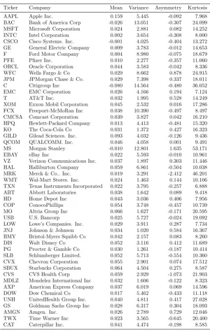
Our empirical exercise is based on a sample composed of 50 most traded stocks belonging to the S&P100 index

between 01/01/2004 and 31/12/2013. The sample goes through periods of growth, recession and economic

recovery, including periods of high and low market volatility, so that we do not restrict the results to a specific

sample characteristic. The sample contains 2516 observations with daily data of returns, computed as the

logarithmic difference of the closing prices. We report in Table 12 descriptive statistics for the sample used in

the paper.

5.2 Results

The presentation of the results is organized in five parts to facilitate the analysis and discussion. Initially, we

discuss the performance of each portfolio strategy in terms of gross returns. Second, we present the results

in terms of portfolio risk measured by the standard deviation of returns. Third, we report the results for the

portfolio turnover. Fourth, we discuss the results in terms of risk-adjusted portfolio returns measured by the SR

for alternative levels of transaction costs. Finally, we report the annualized performance fee that a risk-averse

investor with quadratic utility adopting a given portfolio policy is willing to pay in order to use the PARA static

covariance specification of Ledoit & Wolf (2004). In each part, we report the results for the portfolio policies

obtained with dynamic covariance models as well as those obtained with static covariance models. To facilitate

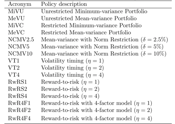
the exposition of results, we refer to each portfolio policy and each covariance model using the acronyms detailed

in Tables 10 and 11 in the Appendix, respectively.

Portfolio gross returns. Table 1 shows the average gross returns (i.e. before transaction costs) obtained by each portfolio policy and the corresponding covariance model used. In the vast majority of instances, average

gross return obtained using dynamic specifications is equal or superior to those obtained with static

specifi-cations. These differences are more substantial for the group of mean-variance portfolio policies. Overall, the

best results in terms are obtained with the RwRs4 policy with the EWMA and ORE specifications (0.11% and

0,10%, respectively).

3

(16)

[image:16.595.66.540.148.276.2]

Table 1: Portfolio gross returns

The table reports the daily average gross return (i.e. before transaction costs) obtained by the each portfolio policy alongside each covariance model over the out-of-sample period. Figures are reported in percentages. The portfolio policies are described in Section 2 whereas the covariance models are described in Section 3. The description of each acronym for the portfolio polices and for the covariance models are reported in Tables 10 and 11.

Strategy MiVU MeVU MiVC MeVC NCMV2.5 NCMV5 NCMV10 VT1 VT2 VT4 RwRS1 RwRS2 RwRS4 RwR4F1 RwR4F2 RwR4F4 Average

Dynamic covariance models

EWMA 0.071 0.076 0.070 0.071 0.071 0.072 0.074 0.062 0.063 0.064 0.066 0.081 0.108 0.059 0.060 0.062 0.071 ORE 0.064 0.065 0.060 0.061 0.061 0.062 0.064 0.062 0.061 0.057 0.064 0.077 0.102 0.059 0.058 0.059 0.065 VECH 0.077 0.083 0.072 0.074 0.073 0.074 0.075 0.062 0.063 0.062 0.064 0.076 0.099 0.060 0.062 0.066 0.071 OGARCH 0.065 0.064 0.056 0.056 0.057 0.058 0.058 0.061 0.059 0.053 0.060 0.064 0.076 0.057 0.057 0.059 0.060 CCC 0.060 0.060 0.062 0.062 0.063 0.063 0.063 0.062 0.062 0.062 0.061 0.066 0.077 0.059 0.059 0.062 0.063 DCC 0.049 0.105 0.074 0.075 0.075 0.076 0.077 0.062 0.062 0.062 0.061 0.066 0.077 0.059 0.059 0.062 0.069 DECO 0.069 0.069 0.060 0.060 0.060 0.060 0.059 0.062 0.062 0.062 0.061 0.066 0.077 0.059 0.059 0.062 0.063 ASYDCC 0.077 0.078 0.073 0.075 0.074 0.075 0.077 0.061 0.062 0.062 0.062 0.075 0.104 0.057 0.057 0.058 0.070 Average 0.066 0.075 0.066 0.067 0.067 0.067 0.068 0.062 0.061 0.061 0.063 0.072 0.090 0.059 0.059 0.061 0.066

Static covariance models

CORR 0.052 0.052 0.055 0.055 0.056 0.056 0.057 0.061 0.058 0.052 0.061 0.066 0.081 0.057 0.055 0.054 0.058 PARA 0.053 0.052 0.055 0.055 0.056 0.057 0.058 0.061 0.059 0.053 0.061 0.067 0.082 0.057 0.056 0.054 0.059 MARKET 0.052 0.052 0.055 0.055 0.056 0.057 0.058 0.061 0.058 0.052 0.061 0.066 0.081 0.057 0.055 0.054 0.058 Average 0.052 0.052 0.055 0.055 0.056 0.057 0.058 0.061 0.058 0.053 0.061 0.067 0.081 0.057 0.055 0.054 0.058

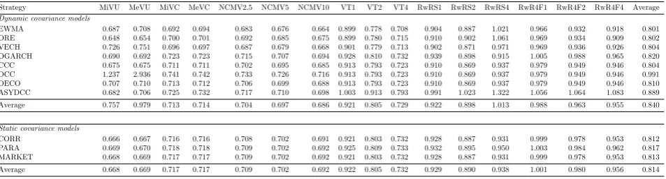
Portfolio standard deviation. Table 2 reports the standard deviation of the gross portfolio returns for each portfolio policy. The comparative results among dynamic and static covariance specifications are rather mixed

according to this performance measure. We observe that the results are similar among policies when using

dynamic covariances or static covariances. An exception is the DCC specification which delivered portfolios

with much higher standard deviations in comparison to other dynamic or static counterparts.

Table 2: Standard deviation of portfolio returns

The table reports the standard deviation of portfolio gross returns obtained by the each portfolio policy alongside each covariance model over the out-of-sample period. Figures are reported in percentages. The portfolio policies are described in Section 2 whereas the covariance models are described in Section 3. The description of each acronym for the portfolio polices and for the covariance models are reported in Tables 10 and 11.

Turnover. The turnover obtained for each portfolio policy is reported in Table 3. The most striking result is that all portfolios obtained with dynamic covariance models displayed much higher turnover in comparison to

those obtained with their static counterparts. For instance, when obtaining portfolios according to the MeVU

[image:16.595.63.540.511.639.2]

(17)

co-variance models is 0.022. We also observe that i) constrained mean-co-variance policies displayed lower turnovers

with respect to unconstrained policies, and ii) policies that ignore off-diagonal covariance elements, such as VT

and RwR policies, also achieved lower turnover with respect all mean-variance policies. It is also interesting to

associate the results in Table 3 with those reported in table 1. In general, we observe that the higher portfolio

average returns obtained with dynamic covariance specifications is usually associated with a higher portfolio

turnover. The most extreme case is that of the DCC specification that has a reasonably superior return (0.069

on average), when compared to the other portfolios, but it was coupled with the highest turnover among all

portfolios observed (0.991 on average). Therefore, even though dynamic specifications with greater structure

[image:17.595.67.539.328.457.2]

are linked to higher average returns, they come associated with much higher portfolio instability.

Table 3: Portfolio turnover

The table reports the portfolio turnover obtained by the each portfolio policy alongside each covariance model over the out-of-sample period. Figures are reported in percentages. The computation of turnovers is described in Section 4. The portfolio policies are described in Section 2 whereas the covariance models are described in Section 3. The description of each acronym for the portfolio polices and for the covariance models are reported in Tables 10 and 11.

Sharpe ratios. We now consider the performance of portfolio policies in terms of risk-adjusted portfolio returns measured by the SR. In order to take into account the impact of portfolio turnovers reported in Table 3 we

compute SR considering portfolio returns net of transaction costs of 0 bp, 20 bp, and 50 bp. In each case, we

indicate with an asterisk the instances in which the SR is statistically different with respect to the one obtained

with the static covariance model PARA according to the bootstrap test proposed in Ledoit & Wolf (2008) at

the level of 5%.

Table 4 reports the SR in the absence of transaction costs. We observe a pattern similar to that of the

average gross returns reported in Table 1, with the specifications EWMA, ORE, and VECH displaying higher

figures than the ones obtained with the static benchmark specification as well as to other dynamic counterparts

when compared within the same portfolio selection policy. We also find that there is no substantial difference

in the risk-adjusted performance of the portfolios obtained with the alternative static covariance models.

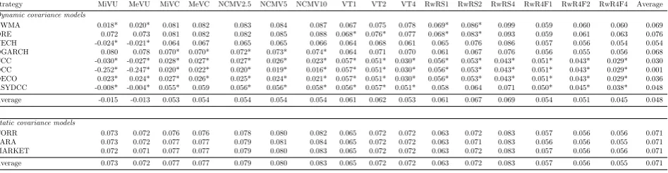
We report in Table 5 the SR when transaction costs of 20 bp are taken into account in the computation of

(18)

[image:18.595.66.539.149.275.2]

Table 4: Sharpe ratios in the absence of transaction costs

The table reports the portfolio SR obtained by the each portfolio policy alongside each covariance model over the out-of-sample period. Figures are reported in percentages. The level of trasaction costs is 0 bp. The computation of portfolio returns net of transaction costs is described in Section 4. The portfolio policies are described in Section 2 whereas the covariance models are described in Section 3. The description of each acronym for the portfolio polices and for the covariance models are reported in Tables 10 and 11. Asterisks indicates the instances in which the SR is statistically different with respect to the one obtained with the static covariance model PARA according to the bootstrap test proposed in Ledoit & Wolf (2008) at the level of 5%

EWMA 0.103 0.107 0.101* 0.103* 0.104* 0.107* 0.111* 0.069 0.081* 0.090* 0.073* 0.092* 0.106* 0.061 0.065* 0.068 0.090 ORE 0.099 0.100* 0.086 0.087 0.088 0.091 0.095 0.069* 0.078* 0.080* 0.070* 0.086* 0.096 0.060* 0.062* 0.065 0.082 VECH 0.106 0.111 0.103* 0.106* 0.106* 0.108* 0.113* 0.069 0.081* 0.087* 0.071* 0.087* 0.102 0.062* 0.066* 0.072* 0.091 OGARCH 0.094 0.093 0.078 0.078 0.080 0.081 0.083 0.066 0.073 0.073 0.064 0.071 0.083 0.057 0.058 0.061 0.075 CCC 0.088 0.088 0.087 0.087 0.089 0.091 0.092 0.067 0.078 0.086 0.067 0.076 0.082 0.060 0.062 0.065 0.079 DCC 0.039 0.036 0.100 0.101 0.103 0.105 0.108 0.067 0.078 0.086 0.067 0.076 0.082 0.060 0.062 0.065 0.077 DECO 0.097 0.097 0.084 0.084 0.085 0.086 0.086 0.067 0.078 0.086 0.067 0.076 0.082 0.060 0.062 0.065 0.079 ASYDCC 0.112* 0.111* 0.101* 0.102* 0.103* 0.106* 0.110* 0.061 0.067 0.078 0.063 0.073 0.078 0.054 0.054 0.054 0.083 Average 0.092 0.093 0.093 0.093 0.095 0.097 0.100 0.067 0.077 0.083 0.068 0.080 0.089 0.059 0.061 0.064 0.082

that Americans spend 21 basis points (bp) in total trading, as a fraction of the total portfolio. We observe that

dynamic covariance specifications delivered higher SR in comparison to those obtained with static covariance

models in very few instances. In most of the cases, the portfolios obtained with static covariance models

outperformed those obtained with dynamic counterparts. This sharp decrease in risk-adjusted performance

net of transaction costs obtained with dynamic covariance models is mostly explained by the presence of a

much higher turnover when compared to static covariance models. In fact, we observe that many SR obtained

with dynamic models turned out to the negative once an intermediate level of transaction costs are taken into

account. In constrast, the SR of portfolio policies obtained with static covariance models were little affected by

the presence of transaction costs.

Table 5: Sharpe ratios based on portfolio returns under transaction costs of 20 bp

EWMA 0.018* 0.020* 0.081 0.082 0.083 0.084 0.087 0.067 0.075 0.078 0.069* 0.086* 0.099 0.059 0.060 0.060 0.069 ORE 0.072 0.073 0.081 0.082 0.082 0.085 0.088 0.068* 0.076* 0.077 0.068* 0.083* 0.093 0.059 0.061 0.063 0.076 VECH -0.024* -0.021* 0.064 0.067 0.065 0.065 0.066 0.064 0.068 0.061 0.065 0.076 0.086 0.057 0.056 0.054 0.054 OGARCH 0.080 0.078 0.070* 0.070* 0.072* 0.073* 0.074* 0.064 0.071 0.070 0.061 0.067 0.076 0.056 0.055 0.056 0.068 CCC -0.030* -0.027* 0.028* 0.027* 0.027* 0.026* 0.023* 0.057* 0.051* 0.030* 0.056* 0.053* 0.043* 0.051* 0.043* 0.029* 0.030 DCC -0.252* -0.247* 0.020* 0.022* 0.020* 0.019* 0.016* 0.057* 0.051* 0.030* 0.056* 0.053* 0.043* 0.051* 0.043* 0.029* 0.001 DECO 0.023* 0.024* 0.027* 0.026* 0.025* 0.024* 0.021* 0.057* 0.051* 0.030* 0.056* 0.053* 0.043* 0.051* 0.043* 0.029* 0.036 ASYDCC -0.008* -0.004* 0.055* 0.059 0.056* 0.056* 0.058* 0.056* 0.057* 0.051* 0.058 0.064 0.071 0.050* 0.045* 0.038* 0.048 Average -0.015 -0.013 0.053 0.054 0.054 0.054 0.054 0.061 0.062 0.053 0.061 0.067 0.069 0.054 0.051 0.045 0.048

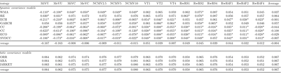
Finally, we report in Table 6 the SR when transaction costs of 50 bp are taken into account, which corresponds

[image:18.595.65.539.574.697.2]

(19)

that dynamic covariance models outperformed static ones in only three instances (RwRS1 and RwRS2 with

EWMA and ORE specifications). In all remaining cases, we find that the risk-adjusted performance of portfolios

obtained with dynamic covariance models are substantially affected by the presence of high transaction costs

[image:19.595.65.539.234.359.2]

and underperformed those obtained with static models.

Table 6: Sharpe ratios based on portfolio returns under transaction costs of 50 bp

EWMA -0.110* -0.108* 0.048* 0.050* 0.049* 0.049* 0.049* 0.062 0.065 0.059 0.062 0.075* 0.087 0.054 0.051 0.045 0.037 ORE 0.030* 0.031* 0.071 0.072 0.072 0.074 0.076 0.065 0.073 0.071 0.063* 0.076* 0.087 0.056 0.057 0.057 0.064 VECH -0.211* -0.210* 0.003* 0.007* 0.001* 0.000* -0.005* 0.054* 0.046* 0.021* 0.055 0.057 0.061 0.047* 0.038* 0.023* -0.001 OGARCH 0.058 0.056 0.057* 0.057* 0.058* 0.059* 0.058* 0.061 0.066* 0.064* 0.055 0.058* 0.065* 0.052 0.049 0.046 0.057 CCC -0.206* -0.199* -0.064* -0.064* -0.068* -0.072* -0.081* 0.038* 0.008* -0.055* 0.038* 0.015* -0.016* 0.035* 0.011* -0.028* -0.044 DCC -0.623* -0.614* -0.100* -0.096* -0.104* -0.109* -0.120* 0.038* 0.008* -0.055* 0.038* 0.015* -0.016* 0.035* 0.011* -0.028* -0.108 DECO -0.089* -0.086* -0.061* -0.062* -0.067* -0.071* -0.078* 0.038* 0.008* -0.055* 0.038* 0.015* -0.016* 0.035* 0.011* -0.028* -0.029 ASYDCC -0.186* -0.173* -0.016* -0.008* -0.017* -0.019* -0.022* 0.048* 0.038* 0.008* 0.048* 0.049* 0.057 0.042* 0.031* 0.012* -0.007 Average -0.167 -0.163 -0.008 -0.006 -0.009 -0.011 -0.015 0.051 0.039 0.007 0.049 0.045 0.039 0.044 0.032 0.012 -0.004

It is also worth analyzing the comparative performance in terms of risk-adjusted returns among alternative

portfolio policies when transaction costs are taken into account. The results reported in Tables 4 to 6 leave three

key messages. First, constrained versions of the mean-variance policies performed better than the unconstrained

ones. This result is in line with those reported in Jagannathan & Ma (2003) and in DeMiguelet al. (2009a). Second, when adopting dynamic covariance models, we find that portfolio policies that ignore off-diagonal

co-variance elements such as the VT and RwR policies of Kirby & Ostdiek (2012) perform better than those than

consider the full covariance structure. This result suggests that the estimation error in off-diagonal covariance

elements plays an important role in the performance of portfolio policies that rely on this type of covariance

specifications. Therefore, if the investor has an a priori preference for a given dynamic covariance specification,

than he or she would be better off by adopting portfolio policies such as the VT and RwR policy in detriment

of mean-variance policies. Third, we find that both mean-variance and VT-RwR policies performed similarly

when considering static covariance specifications.

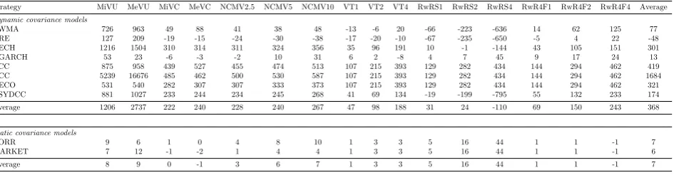
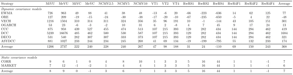
Performance fee for a risk-averse investor with quadratic utility. We report in Tables 7, 8, and 9 the annualized performance fee that a risk-averse investor with quadratic utility and risk aversion coefficientγ= 1

adopting a given portfolio policy is willing to pay in order to employ the PARA static covariance specification

of Ledoit & Wolf (2004) under the presence of 0 bp, 20 bp, and 50 bp transaction costs, respectively. Negative

(positive) figures suggest that the pair portfolio policy/covariance model outperform (underperform) the pair

(20)

those reported in Tables 1 to 6. We find that under the absence of transaction costs, the investor is willing to pay

an average of 28 bp per year on average across portfolio policies and covariance specifications in order to adopt

dynamic covariance models. This result is expected, since dynamic models outperformed static counterparts in

terms of risk-adjusted returns in the absence of transaction costs. However, we observe the opposite result once

we consider the impact of transaction costs. The results in Table 8 reveal that in the presence of transaction

costs of 20 bp, the investor is willing to pay an average annual fee of 368 bp in order to switch to the PARA static

covariance specification. This figure is further increased to an average of 966 bp when the level of transaction

[image:20.595.60.541.311.433.2]

costs is 50 bp.

Table 7: Performance fee to switch to the static PARA covariance specification in the absence of transaction costs

The table reports the performance fee that a risk-averse investor with quadratic utility adopting a given portfolio policy is willing to pay in order to use the PARA static covariance specification of Ledoit & Wolf (2004). Figures are reported in annualized basis points. The level of trasaction costs is 0 bp. The portfolio policies are described in Section 2 whereas the covariance models are described in Section 3. The description of each acronym for the portfolio polices and for the covariance models are reported in Tables 10 and 11.

EWMA 38 213 -117 -75 -129 -136 -137 -32 -53 -75 -79 -250 -662 -5 17 45 -90 ORE -41 37 -60 -54 -65 -72 -83 -20 -28 -30 -67 -233 -625 -8 -4 7 -84 VECH 81 227 -23 -9 -30 -27 -17 -17 -21 -28 -30 -84 -265 -8 -5 -25 -18 OGARCH -16 -37 -66 -62 -64 -56 -41 -2 -15 -28 0 0 35 1 -2 0 -22 CCC -75 3 -83 15 -82 -76 -61 -9 -43 -104 27 64 74 37 65 75 -11 DCC 681 3348 -248 -243 -249 -237 -216 -9 -43 -104 27 64 74 37 65 75 189 DECO -68 -51 -223 -186 -209 -193 -166 -9 -43 -104 27 64 74 37 65 75 -57 ASYDCC -88 35 -174 -146 -182 -181 -179 -9 -47 -125 -57 -264 -802 10 26 42 -134 Average 64 472 -124 -95 -126 -122 -113 -13 -37 -75 -19 -80 -262 13 28 37 -28

CORR 13 11 2 1 4 9 11 1 3 4 5 16 42 1 1 -1 8

MARKET 7 12 -1 -1 2 4 5 1 3 4 5 16 42 1 1 -1 6 Average 10 11 0 0 3 7 8 1 3 4 5 16 42 1 1 -1 7

Table 8: Performance fee to switch to the static PARA covariance specification in the presence of 20 bp transaction costs

The table reports the performance fee that a risk-averse investor with quadratic utility adopting a given portfolio policy is willing to pay in order to use the PARA static covariance specification of Ledoit & Wolf (2004). Figures are reported in annualized basis points. The level of transaction costs is 20 bp. The portfolio policies are described in Section 2 whereas the covariance models are described in Section 3. The description of each acronym for the portfolio polices and for the covariance models are reported in Tables 10 and 11.

EWMA 726 963 49 88 41 38 48 -13 -6 20 -66 -223 -636 14 62 125 77 ORE 127 209 -19 -15 -24 -30 -38 -17 -20 -10 -67 -235 -650 -5 4 22 -48 VECH 1216 1504 310 314 311 324 356 35 96 191 10 -1 -144 43 105 151 301 OGARCH 53 23 -6 -3 -2 10 31 6 2 -8 4 7 45 9 17 24 13 CCC 875 958 439 527 455 474 513 107 215 393 129 282 434 144 294 462 419 DCC 5239 16676 485 462 500 530 587 107 215 393 129 282 434 144 294 462 1684 DECO 531 540 282 307 307 333 373 107 215 393 129 282 434 144 294 462 321 ASYDCC 881 1027 233 244 234 245 268 41 69 134 -19 -199 -795 55 132 233 174 Average 1206 2737 222 240 228 240 267 47 98 188 31 24 -110 69 150 243 368

CORR 9 6 1 0 4 8 10 1 3 3 5 16 44 1 1 -1 7

[image:20.595.67.540.546.669.2]

(21)

[image:21.595.60.540.146.269.2]

Table 9: Performance fee to switch to the static PARA covariance specification in the presence of 50 bp transaction costs

The table reports the performance fee that a risk-averse investor with quadratic utility adopting a given portfolio policy is willing to pay in order to use the PARA static covariance specification of Ledoit & Wolf (2004). Figures are reported in annualized basis points. The level of transaction costs is 50 bp. The portfolio policies are described in Section 2 whereas the covariance models are described in Section 3. The description of each acronym for the portfolio polices and for the covariance models are reported in Tables 10 and 11.

EWMA 726 963 49 88 41 38 48 -13 -6 20 -66 -223 -636 14 62 125 77 ORE 127 209 -19 -15 -24 -30 -38 -17 -20 -10 -67 -235 -650 -5 4 22 -48 VECH 1216 1504 310 314 311 324 356 35 96 191 10 -1 -144 43 105 151 301 OGARCH 53 23 -6 -3 -2 10 31 6 2 -8 4 7 45 9 17 24 13 CCC 875 958 439 527 455 474 513 107 215 393 129 282 434 144 294 462 419 DCC 5239 16676 485 462 500 530 587 107 215 393 129 282 434 144 294 462 1684 DECO 531 540 282 307 307 333 373 107 215 393 129 282 434 144 294 462 321 ASYDCC 881 1027 233 244 234 245 268 41 69 134 -19 -199 -795 55 132 233 174 Average 1206 2737 222 240 228 240 267 47 98 188 31 24 -110 69 150 243 368

CORR 9 6 1 0 4 8 10 1 3 3 5 16 44 1 1 -1 7

MARKET 7 12 -1 -2 1 4 4 1 3 3 5 16 44 1 1 -1 6 Average 8 9 0 -1 3 6 7 1 3 3 5 16 44 1 1 -1 7

6 Concluding Remarks

The literature still lacks consensus regarding what is the best way to model the covariance matrix of asset

returns for high dimensional portfolio selection problems. This work adds to this discussion by comparing the

most popular alternatives in a realistic scenario in which i) there exists many assets, ii) transaction costs are

taken into account, and iii) there is frequent portfolio re-balancing. We find that in the absence of transaction

costs, dynamic covariance models outperform static counterparts in terms of average gross returns as well as in

terms of risk-adjusted returns. On average, Sharpe ratios obtained with dynamic covariance models are 12%

higher than those obtained with static covariance models, and the pairwise differences are statistically significant

in many instances. However, as we move to more realistic scenarios in which transaction costs are properly

taken into account, we find that static covariance models clearly outperform in the vast majority of instances.

Specifically, Sharpe rations based on portfolio returns net of transaction costs of 20 basis points (bp) are 48%

higher when static covariance models are adopted in comparison to those obtained with dynamic models. This

difference in risk adjusted performance becomes even higher when transaction costs of 50 bp are considered.

A closer examination reveals that these differences in risk-adjusted performance are mainly driven by a much

(22)

[image:22.595.147.443.110.320.2]

Appendix

Table 10: Portfolio selection policies and their respectrive acronyms

Acronym Policy description

MiVU Unrestricted Minimum-variance Portfolio MeVU Unrestricted Mean-variance Portfolio MiVC Restricted Minimum-variance Portfolio MeVC Restricted Mean-variance Portfolio

NCMV2.5 Mean-variance with Norm Restriction (δ= 2.5%) NCMV5 Mean-variance with Norm Restriction (δ= 5%) NCMV10 Mean-variance with Norm Restriction (δ= 10%) VT1 Volatility timing (η= 1)

VT2 Volatility timing (η= 2) VT4 Volatility timing (η= 4) RwRS1 Reward-to-risk (η= 1) RwRS2 Reward-to-risk (η= 2) RwRS4 Reward-to-risk (η= 4)

RwR4F1 Reward-to-risk with 4-factor model (η= 1) RwR4F2 Reward-to-risk with 4-factor model (η= 2) RwR4F4 Reward-to-risk with 4-factor model (η= 4)

Table 11: Covariance models and their respective acronyms

Acronym Covariance model description

CORR Shrinkage method with constant correlation target PARA Shrinkage method with identity matrix target MARKET Shrinkage method with market model target EWMA Exponentially Weighted Moving Average ORE Optimal Rolling Estimator

VECH Scalar VECH OGARCH Ortoghonal GARCH

CCC Constant Conditional Correlation DCC Dynamic Conditional Correlation

[image:22.595.153.442.360.514.2]

(23)

[image:23.595.148.449.178.651.2]

Table 12: Descriptive statistics

(24)

References

Alexander, Carol. 2001. Orthogonal garch.Mastering risk,2_{, 21–38.}

Bauwens, Luc, Laurent, S´ebastien, & Rombouts, Jeroen VK. 2006. Multivariate GARCH models: a survey. Journal of applied econometrics,21(1), 79–109.

Becker, Ralf, Clements, AE, Doolan, MB, & Hurn, AS. 2014. Selecting volatility forecasting models for portfolio allocation purposes. International Journal of Forecasting.

Bollerslev, Tim. 1990. Modelling the coherence in short-run nominal exchange rates: a multivariate generalized ARCH model. The Review of Economics and Statistics, 498–505.

Bollerslev, Tim, Engle, Robert F, & Wooldridge, Jeffrey M. 1988. A capital asset pricing model with time-varying covariances. The Journal of Political Economy, 116–131.

Cappiello, Lorenzo, Engle, Robert F, & Sheppard, Kevin. 2006. Asymmetric dynamics in the correlations of global equity and bond returns. Journal of Financial econometrics,4_{(4), 537–572.}

Carhart, Mark M. 1997. On persistence in mutual fund performance. The Journal of finance,52(1), 57–82.

Della Corte, Pasquale, Sarno, Lucio, & Thornton, Daniel L. 2008. The expectation hypothesis of the term structure of very short-term rates: Statistical tests and economic value. Journal of Financial Economics, 89(1), 158–174.

DeMiguel, Victor, Garlappi, Lorenzo, Nogales, Francisco J, & Uppal, Raman. 2009a. A generalized approach to portfolio optimization: Improving performance by constraining portfolio norms. Management Science,55(5), 798– 812.

DeMiguel, Victor, Garlappi, Lorenzo, & Uppal, Raman. 2009b. Optimal versus naive diversification: How inefficient is the 1/N portfolio strategy? Review of Financial Studies,22_{(5), 1915–1953.}

DeMiguel, Victor, Nogales, Francisco J, & Uppal, Raman. 2014. Stock return serial dependence and out-of-sample portfolio performance. Review of Financial Studies,27(4), 1031–1073.

Engle, Robert. 2002. Dynamic conditional correlation: A simple class of multivariate generalized autoregressive conditional heteroskedasticity models. Journal of Business & Economic Statistics,20(3), 339–350.

Engle, Robert, & Colacito, Riccardo. 2006. Testing and valuing dynamic correlations for asset allocation.Journal of Business & Economic Statistics,24(2).

Engle, Robert, & Kelly, Bryan. 2012. Dynamic equicorrelation. Journal of Business & Economic Statistics,30(2), 212–228.

Engle, Robert, & Mezrich, Joseph. 1996. Garch for Groups: A round-up of recent developments in Garch techniques for estimating correlation. RISK,9_{, 36–40.}

Engle, Robert, & Sheppard, Kevin. 2008. Evaluating the specification of covariance models for large portfolios.New York University, working paper.

Engle, Robert F, Shephard, Neil, & Sheppard, Kevin. 2008. Fitting vast dimensional time-varying covariance models.

Fama, Eugene F, & French, Kenneth R. 1992. The cross-section of expected stock returns. the Journal of Finance,

47(2), 427–465.

Fleming, Jeff, Kirby, Chris, & Ostdiek, Barbara. 2001. The economic value of volatility timing. The Journal of Finance,56(1), 329–352.

Fleming, Jeff, Kirby, Chris, & Ostdiek, Barbara. 2003. The economic value of volatility timing using realized volatility. Journal of Financial Economics,67(3), 473–509.

Foster, Dean P, & Nelson, Daniel B. 1996. Continuous Record Asymptotics for Rolling Sample Variance Estimators. Econometrica,64_{(1), 139–74.}

French, Kenneth R. 2008. Presidential address: The cost of active investing. The Journal of Finance,63(4), 1537– 1573.

(25)

Han, Yufeng. 2006. Asset allocation with a high dimensional latent factor stochasticvolatility model. Review of Financial Studies,19(1), 237–271.

Jagannathan, Ravi, & Ma, Tongshu. 2003. Risk Reduction in Large Portfolios: Why Imposing the Wrong Constraints Helps. The Journal of Finance,58(4), 1651–1684.

Kirby, Chris, & Ostdiek, Barbara. 2012. It’s all in the timing: simple active portfolio strategies that outperform naive diversification. Journal of Financial and Quantitative Analysis,47(02), 437–467.

Kolm, Petter N, Tütüncü, Reha, & Fabozzi, Frank J. 2014. 60 Years of portfolio optimization: Practical challenges and current trends. European Journal of Operational Research,234(2), 356–371.

Ledoit, Oliver, & Wolf, Michael. 2008. Robust performance hypothesis testing with the Sharpe ratio. Journal of Empirical Finance,15_{(5), 850–859.}

Ledoit, Olivier, & Wolf, Michael. 2003a. Honey, I shrunk the sample covariance matrix. UPF Economics and Business Working Paper.

Ledoit, Olivier, & Wolf, Michael. 2003b. Improved estimation of the covariance matrix of stock returns with an application to portfolio selection. Journal of empirical finance,10(5), 603–621.

Ledoit, Olivier, & Wolf, Michael. 2004. A well-conditioned estimator for large-dimensional covariance matrices. Journal of multivariate analysis,88(2), 365–411.

Markowitz, Harry. 1952. Portfolio selection*. The journal of finance,7_{(1), 77–91.}

Merton, Robert C. 1980. On estimating the expected return on the market: An exploratory investigation.Journal of Financial Economics,8(4), 323–361.

Olivares-Nadal, Alba V, & DeMiguel, Vıctor. 2015. A Robust Perspective on Transaction Costs in Portfolio Optimization.

Pooter, Michiel de, Martens, Martin, & Dijk, Dick van. 2008. Predicting the daily covariance matrix for s&p 100 stocks using intraday data: But which frequency to use? Econometric Reviews,27(1-3), 199–229.

Silvennoinen, Annastiina, & Ter¨asvirta, Timo. 2009. Multivariate GARCH models. Pages 201–229 of: Handbook of financial time series. Springer.

Thornton, Daniel L, & Valente, Giorgio. 2012. Out-of-sample predictions of bond excess returns and forward rates: An asset allocation perspective. Review of Financial Studies,25_{(10), 3141–3168.}