Asset Pricing Models: Implications for Expected Returns and Portfolio Selection

NBER WORKING PAPER SERIES

ASSET PRICING MODELS: IMPLICATIONS FOR EXPECTED RETURNS AND

PORTFOLIO SELECTION

A. Craig MacKinlay Lubos Pastor

Working Paper 7162

http://www.nber.org/papers/w7 162

NATIONAL BUREAU OF ECONOMIC RESEARCH 1050 Massachusetts Avenue

Cambridge, MA 02138 June 1999

Wethank Bruce Grundy, Ravi Jagannathan, Rob Stambaugh, and the participants at the Yale School of Management Asset Pricing Conference and at the finance seminars at Carnegie Mellon University, Columbia University, Copenhagen Business School, the University of Alberta, the University of Chicago, the University of Frankfurt, Vanderbilt University, the Washington State University, and Wharton for helpful comments. Research support from the Rodney White Center for Financial Research (MacKinlay) is gratefully acknowledged. All opinions expressed are those of the authors and not those of the National Bureau of Economic Research.

© 1999 by A. Craig MacKinlay and Lubos Pastor. All rights reserved. Short sections of text, not to exceed two paragraphs, may be quoted without explicit permission provided that full credit, including © notice, is

Asset Pricing Models: Implications for Expected Returns and Portfolio Selection A. Craig MacKinlay and Lubos Pastor NBER Working Paper No. 7162 June 1999

JELNo. Gi

ABSTRACT

Implications of factor-based asset pricing models for estimation of expected returns and for portfolio selection are investigated. In the presence of model mispricing due to a missing risk factor, the mispricing and the residual covariance matrix are linked together. Imposing a strong form of this

link leads to expected return estimates that are more precise and more stable over time than

unrestricted estimates. Optimal portfolio weights that incorporate the link when no factors are observable are proportional to expected return estimates, effectively using an identity matrix as a covariance matrix. The resulting portfolios perform well both in simulations and in out-of-sample comparisons.

A. Craig MacKinlay Lubos Pastor

Finance Department Finance Department

Wharton School Wharton School

University of Pennsylvania University of Pennsylvania Philadelphia, Pa 19104-6367 Philadelphia, PA 19104-6367

and NBER _{lubos23@wharton.upenn.edu}

1 Introduction

Linear factor-based asset pricing models have solid theoretical foundations in finance fol-lowing the work of Merton (1973) and Ross (1976). If a factor-based pricing model holds exactly it provides simple guidelines for estimation of expected returns and for portfolio selection. Expected asset returns are linearly related to the assets' covariances with the

un-derlying factors, and the mean-variance efficient portfolio of all risky assets can be formed by

combining the factor-mimicking portfolios.1 However, recent empirical literature questions

the usefulness of factor-based pricing models as a mainstay in finance, since these models do

not seem to fully explain the cross section of average returns.2

This paper evaluates the usefulness of factor-based models from a different perspective. Instead of testing the validity of these models, the paper considers a factor-based _pricing model in which mispricing is present. The key assumption is that model mispricing is due to an omitted risk factor. Under this assumption of an exact factor structure, the paper develops implications for estimation of expected returns and for portfolio selection. The usefulness of imposing an exact factor structure is assessed by comparing the expected return estimates and portfolios obtained by invoking these implications to their alternative counterparts.

Suppose that asset returns are generated by a linear (K + 1)-factor pricing model, but only the returns on K factors are observed. In a model that uses the K observed factors only, the (K + l)8t factor is omitted, which results in asset mispricing. Because the mispricing of the K-factor model is due to an omitted factor, there is a relation between the mispricing and the residual covariance matrix from the K-factor model. In the absence of such a relation,

mispriced assets could be collected together to form asymptotic arbitrage opportunities. In this paper, the relation between the mispricing and the residual covariance matrix is

imposed as a restriction in the estimation of the mispricing component of expected return and in portfolio selection.

It is a common practice in finance to estimate expected return and mispricing separately

for each asset. In this paper, the mispricing vector is estimated jointly for a number of

assets. The returns on the other assets are related to an asset's mispricing through the link of the mispricing vector to a common residual covariance matrix. Since covariances can be estimated more precisely than means (see Merton, 1980), the restricted mean estimators that

incorporate the link can be quite precise. Simulations and empirical analysis confirm that this 'See Grinblatt and Titman (1987), Huberman and Kandel (1987), Huberman, Kandel, and Stambaugh (1987), and Jobson and Korkie (1985) for resnits concerning the equivalence between exact arbitrage pricing and the mean-variance efficiency of a portfolio of factor-mimicking portfolios.

2See for example Lakonishok, Shleifer, and Vishny (1994), MacKinlay (1995), and Daniel and Titman

is indeed the case. In simulations, the expected return estimates that incorporate the link are more precise than both sample means and the James-Stein shrinkage estimators of the mean,

unless the sample size is large. With any misspecification, the unbiased sample means become

more precise in sufficiently large samples. In empirical analysis, the restricted expected

return estimates are economically reasonable and more stable over time than both historical averages and grand means of asset returns. Comparisons of the restricted estimators with their alternatives reveal the usefulness of imposing the factor structure.

The link between the means and covariances has striking implications for portfolio selec-tion. A strong form of the link when no factors are observable leads to a simplification in which the identity matrix can be used in place of the covariance matrix when calculating the tangency portfolio weights. In simulations, the identity covariance matrix is compared

to the sample covariance matrix as well as to the true covariance matrix that is used to

generate returns. These comparisons are conducted based on the true Sharpe ratios of the optimal portfolios constructed using the various covariance matrices, Without exception,

the identity matrix outperforms not only the sample covariance matrix, but also the true

covariance matrix, regardless of what estimator of the mean is used. This result appears to be robust to violations of the underlying assumptions. Using the identity matrix effectively links the estimator of the expected return to the covariance matrix, whereas using the true covariance matrix does not. The gains from using the identity matrix are especially large when a relatively imprecise estimator of expected excess return is used, such as the usual sample mean. Portfolios constructed using the identity covariance matrix also perform_very

well in out-of-sample empirical analysis.

This paper is also related to the literature on the construction of factors for linear asset

pricing models. In empirical research, factors constructed using two very different techniques

have been widely used. One factor-construction technique extracts common factors from the

sample covariance matrix of returns using factor analysis or principal components (e.g.,

Connor and Korajczyk (1986), Roll and Ross (1980)). Another factor-building technique assigns assets to several groups based on certain characteristics so that sample mean returns differ across the groups. The difference in average returns across the groups can serve as a factor in a multifactor pricing relation. This second approach is used to build the Fama and

French (1993) SMB and HMLfactors.3 _{The two factor-building techniques lead to different}

factors since they use different information to construct the factors. The Connor—Korajczyk

3The SMB factor is the return of a portfolio of low market value of equity firms minus the return ofa portfolio of high market value of equity firms. The HV1L factor is the return of a portfolio of firms with high book value to market value of equity ratios minus the return of a portfolio of firms with low book value to market value of equity ratios.

factors are obtained from the information in sample variances and covariances, whereas the Fama—French factors are obtained from the information in sample means. The approach

used in this paper can be interpreted as a mixture of the two techniques. Since the mean return is explicitly linked to the covariance matrix of returns, factors are built using the

sample information about both the means and the covariances.

The paper proceeds as follows. Section 2 presents the factor model structure used in

the analysis, including the link between the mispricing and the residual covariance matrix. Section 3 discusses the application of the "link-based" approach to estimation of expected

returns and to portfolio selection. Section 4 contains some simulation results illustrating

the usefulness of imposing the link. Section 5 uses actual stock market data to compare the link-based portfolio selection strategy with some traditional strategies. Section 6 concludes.

2 Linear Factor-Based Asset Pricing Models.

Consider a linear factor model for the returns on N given assets. LetZt denote the vector of

returns on these N assets in period t, with mean u and covariance matrix V. Throughout

the paper, the term "return" on a given asset denotes the asset's return in excess of the risk-less rate, unrisk-less the asset is a zero-investment position. For a set of K factor portfolios, the

following linear relation between the asset returns and the factor portfolio returns is assumed:

a + BZKt + Et,

₍₁₎

0, E[€']

,

(2)

E[zKt] = _{/-K, E[(zKt}—

/1K)(ZKt—

K,

_{Cov[zKt, €]} 0. ₍₃₎

B is the N x K matrix of factor sensitivities, ZKt is the K-vector of factor portfolio returns in period t, a is the N-vector of mispricings, and Et is the N-vector of disturbances, Assume that the factor portfolios are not linear combinations of the N assets, so that is full rank.

An exact K-factor pricing relation implies that each element of the mispricing vector a equals zero. If exact pricing does not hold due to a missing factor, then a is non-zero

and related to the residual covariance matrix .

The relation between a and can be

developed using the optimal orthogonal portfolio discussed in MacKinlay (1995). This is the unique portfolio constructed from the population of assets which is optimal since it can be combined with the factor portfolios to form the tangency portfolio and is orthogonal to

the factor portfolios.4 The optimal orthogonal portfolio is denoted by h. The usefulness

of portfolio h comes from the fact that when it is added to the K-factor model in (1),

the intercept a vanishes and the factor sensitivity matrix B is not altered. The optimality

property leads to the intercept vanishing, and the orthogonality condition leads to B being unchanged. Since the mispricing vanishes when h is added to the K factors, h can be thought of as the omitted (K + i)8tfactorin a linear asset pricing model. Adding the omitted factor,

Zt =

BZKt + /3hZht + Ut, ₍₄₎

E[u]

0, E[UtUt'] =

,

₍₅₎

E[zht] = bth, E[(zht —

/th)]

o,

(6)

Cov[zKt, Ut] = 0, Cov[zht, Ut] = 0, ₍₇₎

where 3,, is the N-vector of assets' sensitivities to the omitted factor h and Zht denotes the

return on portfolio h at time t. The link between a and _{results from comparing (1) and}

(4). Taking the unconditional expectations in both equations,

a =

/3h1-'h, (8)

and by equating the variance of with the variance of /3hZht + Ut,

/I3hI3YT +

aaOh

+ ₍₉₎

where 8h denotes ,

the inverse of the squared Sharpe ratio of portfolio h. Equation (9)

links the model mispricing a to the residual covariance matrix ,_given an assumption about

the structure of t. For example, the derivation of APT in Ross (1976) assumes that is

diagonal. If _{is unrelated to a, asymptotic arbitrage opportunities exist. MacKinlay (1995)}

presents examples of such opportunities and illustrates that, in the absence of the link,

unrealistic risk—return tradeoff positions can be created with even a small number of assets.

3 Expected Returns and Portfolio Selection.

This section extends the analysis of Section 2 to develop implications for estimation of expected returns and for portfolio selection. The environments with one factor and with

multiple factors are analyzed in separate subsections.

3.1 One factor.

A statistical model in which asset returns are generated by one factor has often been employed

in finance since the introduction of the diagonal model by Sharpe (1963) and its application by 'Ieynor and Black (1973). In this section, asset returns are assumed to be generated by a one-factor model, but the factor h is assumed to be unobserved.5 This model corresponds

to that presented in equations (4) through (7) for K 0:

Zt _{/3hZht + Ut, (10)}

E[u] =

0, E[UtUt'] = Cov[zht,UtI = 0. ₍₁₁₎

Since Zht is unobserved, the model used in the analysis corresponds to that presented in

equations (1) through (2) for K 0:

a + Et,

₍₁₂₎

0 and _E[cjcj] >1. ₍₁₃₎

Following the argument from the end of the previous section, (10) through (13) imply

QE8h + Thus, the mean a appears in the covariance matrix of returns. This observation

is used in the estimation of expected returns and in portfolio selection.

The usual arbitrage pricing theory assumption in a one-factor model would be that the

elements of Ut are sufficiently uncorrelated so that, as the number of assets in a portfolio goes

to infinity, the residual variance of the portfolio goes to zero. Such an assumption does not put sufficient structure on 1 for the purposes of this paper. This paper makes the stronger assumption that cF is diagonal and proportional to the identity matrix:

o-21 ₍₁₄₎

This assumption in combination with the relation in (9) is referred to as a "strong form" of the link between a and _{While the assumption may appear strong, this paper demonstrates}

5One might think of the true market portfolio as the unobserved factor. In that case, this framework addresses some of the concerns in Roll (1977). However, our assumptions about the structure of cI are not required to obtain the CAPM.

that the payoff from the rigid structure delivered by this assumption typically dominates the cost due to possible misspecification.

A reasonable alternative way of specifying

would be to make it diagonal but not

necessarily proportional to the identity matrix, such as in Sharpe's diagonal model. Such an

approach would account for potential differences across the N assets in the residual variances from the model that includes the unobserved factor. This could be useful particularly if the N

assets are fundamentally different from each other, such as if bond portfolios are mixed with stock portfolios. However, this approach would come at the expense of having to estimate

additional (N —_{1) parameters when the model is taken to the data. Simulation results not}

reported here have shown that the benefits of relaxing the assumption (14) when the N

assets belong to the same broad asset class (for example, when all the assets are individual

stocks or stock portfolios) are minimal, if any. Since our subsequent analysis uses assets from

the same class, the assumption that is proportional to the identity matrix is maintained throughout the paper.

3.1.1 Estimation

of expected return.

For estimation purposes, the disturbances c in (12) are assumed to be normally distributed.

Although returns on many assets appear to depart from normality to some extent, this

assumption allows convenient estimation of the parameters restricted by the link using the maximum likelihood procedures. The likelihood function is proportional to

L(, 0h,

._{, ZT)}

'Oh + a2I_T/2 exp

(Zt —

_)'(Q'Oh

+ a21)'(zt —

(15) The maximum likelihood estimators of c, 0h, and a2 are obtained by maximizing the joint log-likelihood function with °h and a2 constrained to be positive. Since closed-form solutions for

the maximum likelihood estimates are not available, a constrained quasi-Newton numerical

procedure is adopted.6

Separately, the model is also estimated conditional on a given value of °h• From a

Bayesian perspective, conditioning on °h is an extreme case of having prior information about the maximum Sharpe ratio. The corresponding results will therefore be informative about the value of having such prior information. To some extent, the value of °h can be viewed as the degree of confidence in the K-factor pricing model. A dogmatic belief in the

6The actual estimation uses Matlab's constrained minimization routine constr, which uses a Sequential Quadratic Programming method. For a detailed exposition of this method, see Matlab's Optimization Toolbox manual.

model, which rules out mispricing, corresponds to °h —*oc (i.e., the Sharpe ratio of portfolio h equal to zero). The other extreme, °h —f0, can be viewed as complete skepticism about

the model, combined with the belief that the maximum Sharpe ratio in the population of assets can be arbitrarily large. A different way of incorporating a degree of belief in an

asset pricing model is proposed by Pastor and Stambaugh (1999) in estimation of expected returns, and by Pastor (1999) in portfolio selection.

In simulations and in empirical analysis, expected return estimates and portfolios ob-tained from the model restricted by the link QcVOh + a21 are compared to alternative

estimates and portfolios that do not impose the restriction. Such a comparison facilitates

judgment of the gains from incorporating the factor structure.

3.1.2

Portfolio selection.

In a mean-variance framework with a riskless asset, the optimal portfolio of the risky assets,

the "tangency portfolio", is the portfolio with the maximum Sharpe ratio among all portfolios

of the N assets. Let XN* denote the N-vector of the tangency portfolio weights. A standard result from mean-variance mathematics is that

=

_(JV't)1Vi,

₍₁₆₎

where t is a conforming vector of ones. Recall from (12) and (13) that, in the model with no observed factors, the mean ji of asset returns Zt is equal to i and the covariance matrix V is equal to _Hence,

XN* = ₍₁₇₎

In simulations and in empirical analysis, the optimal weights are computed as in (17), using different estimators of c and

.

Given the structure of from (9), the inverse of equals (see Morrison (1990), page 69)

=

_('Oh

_{+ )_i}

—

(18)

1

+ Ohc'1Q

Substituting the inverse of I into (17), the weight vector simplifies to

When the link between c and is imposed in the strong form cJ a21, the restricted tangency portfolio weight vector is

xpj =

(t'a—'c. (20)

This simple result is striking. Imposing one-factor structure when no factor is observed

implies that the tangency portfolio weights are proportional to the vector of mean returns.

There are two possible sources of gains from using the restricted estimator of the tangency

portfolio weight vector relative to an unrestricted estimator. First, the restricted estimator of the mean is likely to be more precise due to including the information in the covariances. Second, imposing a strong form of the link between c and leads to the simplified expression

in (20). This expression implies that, in this framework with one unobserved factor, imposing the link is equivalent to using an identity covariance matrix in computing the optimal weights.

One need not use the restricted estimator of c to realize the gains from this second source.

Plugging in the identity matrix for the covariance matrix in (17) links together the mean

and the covariance matrix for any estimator of c. The importance of both sources of gains is illustrated in simulations in Section 4.

3.2 Multiple factors.

In the multifactor case, an exact (K + 1)-factor pricing relation with K observed factors

is examined. The analysis is presented for the two-factor case (K 1), but the extension

for K > 1 is straightforward. Let p denote the observed factor portfolio, and z, denote its return at time t. The two-factor linear model is:

Zt

O +

j3z + Et

₍₂₁₎

E[c] =

0, cc'Oh

+

(22)

Recall that the second factor can be thought of as the optimal orthogonal portfolio h that annihilates c upon its addition to the model.

3.2.1 Estimation of expected return.

The expected return for the N assetsis

The expected return has two components, the mispricing vector with respect to the K-factor

model, ,

and _{the factor-related component, /3t1. Thelink between the mispricing and the}

residual covariance matrix can be used in estimating ü. As in section 3.1.1, by imposinga

rigid structure on as in (14), maximum likelihood can be employed to estimate the model parameters conditional on the returns on the factor portfolio p. The maximum likelihood

estimate of c is _{an estimate of the mispricing component of the expected return. This} estimate can be combined with an estimate of the factor-related component to obtain an

estimate of the expected return.

3.2.2 Portfolio selection.

Suppose that the set of investable assets consists of N assets and K 1 traded factor

portfolios. The objective of mean-variance portfolio selection is to find the tangency portfolio

of the N + 1 assets. The process of choosing the tangency portfolio can be broken down into two stages, as pointed out by Treynor and Black (1973) and Gibbons. Ross, and Shanken

(1989), among others. In the first stage, the so-called active portfolio of the N assets is

constructed. In the second stage, this active portfolio is combined with the factor portfolio to form the tangency portfolio.7 In subsequent analysis, a modified version of this active portfolio is employed. The active portfolio is modified to be uncorrelated with the factor portfolio by including the factor portfolio as its component. The resulting modified active

portfolio can be viewed as the optimal orthogonal portfolio in the universe of the N + 1

assets. The weights in the active portfolio will be shown to depend on the mispricing and not on the mean or variance of the observed factor. The optimal mix of the active and factor portfolios depends on the factor portfolio's mean and variance.

Let XN+ denote the (N + 1)-vector of weights in the tangency portfolio, whose first N

elements represent the weights in the N assets and the (N + i)st element represents the

weight in the factor portfolio. It is shown in the appendix that

XN+ =

c1 , ₍₂₄₎

—YQ +

where c1 is _{a normalizing constant such that tXN+}

_{1. When the structure =}

ctcVO,,

+ 't

from Section 2 is incorporated and substituted into (24), the tangency portfolio weights_can

7When more than one traded factor portfolio is available, the second stage splits into two_{steps. One} step is choosing the optimal portfolio of the factor portfolios and the second step is choosing the mix of that optimal portfolio with the active portfolio.

be written as

0

Cl

+

, (25)

—c2I'

Up

wherec2 _1/(1+ 9hc'1c).8 Consider an active portfolio a:

Xa C3 , ₍₂₆₎

—/-'

where _{c3 is a normalizing constant such that /!Xa} = 1. _{From (25), the tangency portfolio}

of the (N + 1) assets can be formed by combining portfolio a and portfolio_{p. (Recall that} portfolio p is the (N+ i)8tasset.) Using the fact that portfolio a is uncorrelated with portfolio

p (since its beta equals zero, i.e., [3' 1]Xa 0), the optimal mix between the portfolios a and

p is particularly simple. The tangency portfolio is formed with the weights /2

in a

and _{in p. Furthermore, because a and p are uncorrelated, the squared Sharpe} ratio of the tangency portfolio is the sum of the squared Sharpe ratios of a and_p.

The active portfolio in (26) does not yet reflect the restrictions imposed by exact factor pricing, since is unrestricted. Restricting _{to be proportional to the identity matrix}

simplifies the active portfolio weights:

c

Xa C4 , ₍₂₇₎

-/

where _{c4 is a normalizing constant such that t'Xa,. 1. The weights on the N assets are}

simply proportional to the mispricing vector. The weight on the factor portfolio makes the active portfolio zero-beta with respect to the factor.

As mentioned earlier, the modified active portfolio a can be viewed as the optimal

or-thogonal portfolio. This portfolio can be added to the K observed factors and cause the mispricing to disappear. As shown in (27), a's weights in the N assets with restricted are proportional to the mispricing vector. Combining the two observations implies that

8lnverting and post-multiplying the result by cgives = = wherec2

empirically constructed factor portfolios whose weights in the N assets are approximately proportional to a should do a good job in bringing the model mispricing close to zero. An example of such empirically constructed factors are the Fama—French SMB and HML fac-tor portfolios described earlier. Both of these portfolios essentially assume long positions in stocks with positive a estimates and short positions in stocks with negative a estimates (where a's are estimated from the market model), so when added as factors to the market portfolio, they bring the mispricing closer to zero than the CAPM.

The previously noted two possible sources of gains from using the exact factor pricing

restrictions for portfolio selection are again present. First, the restricted estimator of the

mispriciug vector a could be more precise. Second, the link between a' and > leads to the

simplified expression in (27).

4 Simulation Results.

This section presents a simulation experiment designed to evaluate the potential gains from linking the means to the covariances. In a simulated environment, the true mean and co-variance matrix are known, which is helpful in assessing the usefulness of their alternative estimators. The analysis with one unobserved factor is applied in two environments. In the first environment, returns are generated by a single unobserved factor, as assumed in the estimation. This environment provides a measure of the maximum gains from imposing the a —> _{link. In the second environment, returns are generated by two unobserved factors, but}

the estimation is again conducted assuming only one unobserved factor. This environment illustrates the benefits of using the restricted framework under a misspecified model.

4.1 Environment I: One-factor return-generating model.

Returns on N 10 assets are generated from a one-factor model:

ZtflhZht+Ut, utN(0,a2IN), zhtN(Rh,a), t 1,...,T.

(28)

The parameters of the simulated environment are specified to correspond approximately to monthly returns. The elements of /3h are evenly spread between 0.5 and 1.5, and a

The moments of the factor portfolio returns are set equal to Rh = %% and

_{a, = /i-' so}

the inverse of the squared Sharpe ratio of the factor portfolio Ii is °h 48. One thousand

samples are generated for three values of T: 60, 120, and 360. The estimation results are reported in Table 1 for expected returns and in Table 2 for portfolio selection.

4.1.1 Expected return.

Four estimators of the expected return vector a are calculated for each asset. The first

estimator is the (nnrestricted) sample average return, denoted by a subscript "n". The second estimator is the James-Stein estimator, snbscripted by "JS". Following Jorion (1986), the James-Stein estimator of the expected return vector is computed as

flJSflWaCMt+(1W) a,

(29)

where & is the vector of sample means of the assets' returns, &CM is _{the average of the} sample means across assets (the grand mean), and

=

mm

(N—2)/T

.

₍₃₀₎

\

whereV is the sample covariance matrix of retnrns. In repeated samples, this shrinkage esti-mator has lower risk than the sample mean.9 The third estiesti-mator is the restricted estiesti-mator rl, obtained by maximizing the likelihood function in (15). The fourth estimator is obtained by maximizing the likelihood conditional on the true value °h _48, and denoted by r2.1° For each estimator, measures of bias and precision are presented. The bias is calculated as the estimate's average deviation from the true expected return. The precision is calculated as the root mean square error (RMSE), the square root of the average squared deviation. All averages are grand means, taken across the 1,000 samples and across the N =10 assets.

Table 1 reports the results for expected returns, all on a monthly basis. The_average

biases are all close to zero, no more than 0.08% for the first restricted estimate with T =60.

The RMSE varies substantially across the four estimators, and the variation is most dramatic

for T 60. The RMSE for the unrestricted estimate is 0.98%. The James-Stein estimator reduces the RMSE to 0.74%, and the first restricted estimator to 0.44%. The RMSE is

further reduced to 0.13% when the value of °h is _{known. The reason behind this reduction} 9For more details, see the references in Jorion (1986).

'°In some samples, the sample mean of the factor returns is negative, although the population mean is positive. In such cases, the restricted mean return estimates are predominantly negative across assets, and the negative mean estimates of the high-mean assets (those with high factor loadings) are larger in absolute value than those of the low-mean assets. To handle this problem without using unobserved information, the signs of the restricted estimates are reversed when their sum across assets is negative (i.e., when the expected return on the estimated global minimum variance portfolio is negative). The sign reversal yields more sensible expected return estimates. The occurrence of the simulated samples with the sign reversal is low, at most 9% with T =60,so the impact of the sign reversal on the results reported in Tables 1 and 3 is low. There is no impact at all on the portfolio selection results in Tables 2 and 4, since reversing the signs of all mean returns has no effect on the tangency portfolio weights.

is that 0h is difficult to estimate precisely, since it enters the likelihood function in (15)

only by multiplying an', which is also being estimated. Estimation error in °h can result in multiplicative estimation error in the estimates of a. The reduction in RMSE becomes less pronounced as T increases, since sample mean is an unbiased estimator, unlike the restricted estimators. However, some reduction is still present for T =360: the RIVISE of the sample

mean is 0.40%, whereas that of the second restricted estimator is only 0.05%.

In an earlier version of the paper, the simulation exercise was also repeated with N =30

assets, leading to the same conclusions. Using the information in the covariances increases

the precision of the expected return estimates, especially for smaller values of T. As T

increases, the gains from restricting the parameters are smaller due to the unbiasedness of the unrestricted estimator. Additional information about the Sharpe ratio of the unobserved factor is very helpful in increasing the precision of the expected return estimates: for T =60,

the mean square error is on average reduced by a factor of about 50.

4.1.2 Portfolio selection.

Portfolio selection is examined next, using the same set of simulated samples. Given the estimates /Tt for the expected return vector and V for the covariance matrix, the vector of tangency portfolio weights can be calculated as

=

(t''t'4.

₍₃₁₎

In a simulated environment, it is natural to compare portfolios based on their true Sharpe

ratios. Let R and V denote the true mean and covariance matrix, respectively. The true

expected excess return of portfolio

is i()

',u, and the true standard deviation is

a() ['V±] .

The true Sharpe ratio is calculated as

Sm = ₍₃₂₎

a(x)

Five different values are considered for the expected return the true value, the

unre-stricted estimate u (the sample mean), the James-Stein estimate JS, the reunre-stricted estimate rl, and the restricted estimate r2. Five different values are used for the covariance matrix

— _the

true value, the unrestricted estimate u (the sample covariance matrix), the restricted

estimate rl, the restricted estimate r2, and the identity matrix. Recall that using the

iden-tity matrix corresponds to imposing the mean—covariance link. For restricted estimates of the mean, using the identity matrix is equivalent to using the restricted covariance matrix.

For the true mean, using the identity is the same as using the true covariance matrix, since the true covariance matrix is chosen such that the simplification of (19) into (20) applies.

For each combination of the mean vector and the covariance matrix, Table 2 reports

the average (monthly) Sharpe ratios across the 1,000 simulations. Below each average, the standard deviation of the 1,000 ratios is reported. Panel A contains the results for T =60.

The value of 0.1351 in the top left corner of the panel is the true maximum Sharpe ratio for the 10 assets, calculated using the true mean and covariance matrix. With the true _mean, the choice of the covariance matrix has a fairly small effect on the tangency portfolio's true Sharpe ratio. However, when the mean is estimated, the choice of the covariance matrix is

much more important. In general, using the sample mean (&) results in poorly behaved portfolios, with average Sharpe ratios of about 0.04. However, when the identity matrix is used as the covariance matrix, the average Sharpe ratio for the sample mean is much higher,

0.1130. This is a striking result with the mean return estimated as the sample average, using the identity matrix is far better than using the true covariance matrix. This finding is

consistent with the importance of the sample interaction between the means and covariances,

and is also observed for the other expected return estimates. The James-Stein estimator

outperforms the sample mean for every covariance matrix, and the highest Sharpe ratio (of 0. 1273) is obtained using the identity matrix. The restricted estimates both outperform the James-Stein estimator for every covariance matrix, and the Sharpe ratio (of 0. 1349) for the identity matrix is very close to the true value.

Note that the results for both restricted estimators are almost identical. This contrasts with the different performance of rl and r2 in the estimation of expected return. The reason

is that what matters for portfolio selection is that the mean estimate be proportional to the true mean, not necessarily equal to it. As mentioned earlier, 9h enters the likelihood

function only by multiplying The estimation error in 9, enters primarily by multiplying all elements of c _by the same scalar, which has no impact on the optimal weights. Since c also enters the likelihood without multiplying °h, the results for ri and r2 can differ. The differences between the results for ri and r2 depend on the importance of the terms

in the likelihood that involve c not multiplied by 0h, and these differences are very small throughout the paper. Hence, the knowledge of the Sharpe ratio of the optimal orthogonal portfolio is not very useful in portfolio selection. Moreover, since portfolio selection does

not depend on °h, the_{difficulty in estimating °h} has no effect on the interesting portfolio implications of the c — _link.

Panel B of Table 2 contains portfolio selection results for T 360. The conclusions are quite similar to those from Panel A, except that the unrestricted estimate shows some improvement. This is not unexpected, since the sample mean is unbiased and its variance

declines as T increases. The James-Stein estimator again outperforms the unrestricted esti-mator, and the highest Sharpe ratios are again achieved by the restricted estimators. As in Panel A, all expected return estimators perform best with the identity matrix, even better than with the true covariance matrix.

In an earlier version of the paper, the simulation exercise has also been repeated with

N 30 and N 80 assets. With the larger values of N, the true Sharpe ratios for the

unrestricted mean estimate are even lower, and the benefits from using the identity matrix

are higher than for N 10. Otherwise, the larger values of N lead to the same conclusion.

There appears to be a substantial payoff in portfolio selection from using the link implied by an exact factor structure, especially when the mean is estimated poorly.

4.2 Environment II: Two-factor return-generating model.

The purpose of analyzing the second environment is to investigate the robustness of the one-factor analysis by examining the effect of imposing the mean-variance link in a misspecified model. The estimation is conducted assuming one underlying factor, although the returns

on N — 10assets are simulated from a two-factor model:

Zt + +

€,

_N(0,

),

z

u), t =

1,...,T. ₍₃₃₎

Recall that the second factor can be thought of as the optimal orthogonal portfolio h that

causes c to disappear upon its addition to the model. Since =_ci&Oh+ a21, the mean and covariance matrix of returns are:

= +

and V =

9h

_{+ 3'a + a21.}

₍₃₄₎

The parameters of the simulation are specified to correspond approximately to monthly

returns. The elements of c are evenly spread between —% and %,_creatingan annualized

spread of 10%. The elements of 3 are evenly spread between 0.5 and 1.5. The elements of c and are randomly paired and the pairs are held fixed across the simulations. The moments

of the factor portfolio p are set to j =

_%

and a 2'

so that the annualized Sharpe ratio of portfolio p is 0.5. Also, °h= 110

and a =

_{%. The}

Sharpe ratios of the factor h underlying and of portfolio p imply that the annualized maximum Sharpe ratio for this simulated environment is 0.6.11 One thousand samples are generated for three values of T: 60, 120, and 360. The estimation results are reported in Table 3 for expected returns and in

Table 4 for portfolio selection.

4.2.1 Expected return.

Four estimators of the expected return vector

i

are _{considered: the unrestricted} estima-tor u, the James-Stein estimaestima-tor JS, the restricted estimaestima-tor rl that incorrectly assumes a one-factor structure, and the restricted estimator r2 conditional on °h 33_{that incorrectly} assumes a one-factor structure. Conditioning on that particular value of 0h in the computa-tion of r2 assumes that the Sharpe ratio of the only (unobserved) factor is equal to the true maximum Sharpe ratio in the two-factor environment)2

Table 3 contains the biases and precisions of the alternative expected return estimators, analogous to Table 1. The average biases are again close to zero, no more than 0.11% for

the restricted estimator r2.13 The RMSE varies substantially across the estimators. For

T =

_{60, the RMSE for the unrestricted estimator is 1.06%, whereas it is only 0.79% for the} James-Stein estimator, 0.54% for the restricted estimator ri, and 0.42% for the restricted estimator r2. As in Table 1, the reduction in RMSE across estimates is less _pronounced for larger values of T. For T = _{360, the RMSE decreases from 0.42% for the unrestricted}

estimate to 0.33% for the second restricted estimate, and iS has a lower RMSE than rl. In an earlier version of the paper, the analysis was repeated with N 30_{assets, leading to} the same conclusions. Despite the misspecification, using the information in the covariances increases the precision of expected return estimates, especially for smaller values of T. As T grows, the gains from imposing the restrictions disappear since the restricted estimators remain biased, unlike the sample means. Additional information about the maximum Sharpe ratio for the whole environment reduces the RMSE, but the reduction is small as the bias sometimes increases when that information is incorporated in a misspecified model.

4.2.2 Portfolio selection.

Portfolio selection is examined next, using the same set of simulated samples. Table 4_reports

the simulation results in the same format as Table 2. Panel A contains the results for T

=

60.

The true maximum Sharpe ratio is 0.1557. In this second environment, using theidentity matrix with the true mean is no longer the same as using the true covariance matrix. The true covariance matrix now has a two-factor structure [see (34)], and the simplifications of

'2The monthly Sharpe ratio corresponding to °h= 33_{is ./i7ãã= 0.17, or 0.6 annualized.}

'3An inspection of the biases for each asset reveals that the biases of the restricted estimators_{can sometimes} be substantial. Although the biases are typically small, for several assets, the bias of r2 exceeds 0.50%. Such a finding is not unexpected, since the model is misspecified. Despite the bias, each asset's RMSE for the restricted estimator is lower than for the unrestricted estimator.

(19) and (20) occur only with a one-factor structure. Using the sample mean always leads

to the lowest Sharpe ratios. This unrestricted estimate performs worst with the sample

covariance matrix and the true covariance matrix, and best with the identity matrix. This result deserves emphasis for two reasons. First, even in a misspecified model, imposing the link implied by the one-factor model leads to substantially higher Sharpe ratios. Second,

as in the first environment, using the true covariance matrix with the unrestricted mean

estimate works quite poorly. Using the identity covariance matrix, which effectively links the covariance matrix to the sample mean, leads to substantial improvement.

We also observe that shrinking the sample means toward the grand mean increases the

true Sharpe ratios. The identity matrix is the best choice for the covariance matrix also with the James-Stein estimator of the mean. Since the restrictions are now misspecified,

the restricted estimators rl and r2 no longer lead to average Sharpe ratios close to the true

maximum. However, their Sharpe ratios still uniformly exceed those obtained using the

sample means, and even the James-Stein estimators. The Sharpe ratios are the lowest when the true covariance matrix is used.

Panel B of Table 4 contains portfolio selection resnlts for T = 360. _{Using the identity}

matrix, the average Sharpe ratio is now higher for the unrestricted estimate than for the

restricted estimates, This is not surprising. As mentioned earlier, the unrestricted estimate is unbiased and converges to the true mean as T increases. In all cases, the identity matrix

continues to be a reasonable choice for the covariance matrix, despite model misspecification

in this two-factor environment. This result highlights the importance of imposing a relation between the mean and the covariance matrix in portfolio selection.

A number of interesting results emerge from the simulations. First, recall that using the

identity covariance matrix imposes a strong link between the mean and the covariance matrix

in a one-factor model with an unobserved factor. In all scenarios with estimated means, the true Sharpe ratios are higher when the identity matrix is used than when the true covariance matrix is used, even in the presence of misspecification. This powerful result supports an important economic role of factor models. Second, portfolio selection can be improved when the estimate of the mean incorporates the information in the covariances. This improvement is present in small and medium samples even when the underlying assumptions are violated. In large samples, the improvement disappears as the variance reduction is more than offset by the bias in the restricted estimates.

The environment analyzed in this subsection illustrates the robustness of the results to model misspecification. Further analysis reveals that the usefulness of linking the mean and

the covariance matrix is also robust to other forms of misspecification. The simulations in both environments have been repeated with less structure imposed on the true

return-generating covariance matrix of uJ4 The results in both environments, not reported here

to conserve space, are similar to those reported in Tables 1 through 4. In an earlier version of the paper, the simulations in both environments have also been repeated for N =30and

N 80, leading to the same conclusions. Across the simulations, the restricted estimates

of the mean are more precise than the unrestricted estimates, and the identity matrix beats the true covariance matrix in portfolio selection for all estimates of the mean. In fact, for the larger values of N, the gains from using the identity covariance matrix in portfolio selection

are even larger.

5 Empirical Illustrations.

This section provides an illustration with actual data of the role that the economic restrictions

of exact factor pricing can play in estimation of expected returns and in portfolio selection. Empirical results are presented for two universes of assets: 10 size-sorted portfolios and 30 individual stocks. For each universe, two scenarios are considered one in which no factors are observed, and the other in which one factor is observed.

5.1 Decile Portfolios

The size decile portfolios are value-weighted portfolios of NYSE, AMEX, and NASDAQ stocks sorted by market capitalization, with an equal number of NYSE stocks in each decile. Excess decile returns are obtained from the CRSP for January 1926 through December 1996 using the one-month Treasury bill return as the risk-free rate.

A monthly series of expected return estimates and optimal portfolio weights is computed

using a "rolling sample approach" for windows of T 60 and T 120 months. The first

sample period for the 120-month window is January 1926 through December 1935. The decile returns from that period are used to estimate expected returns and calculate portfolio weights, and the return on the resulting portfolio is recorded for January 1936. The 120-month window is then rolled forward so that January 1926 is dropped and January 1936 is added to the sample, and the portfolio return is recorded for February 1936. This_process is continued until a time series of observations through December 1996 is built. The same approach is used for the 60-month window, except that the January 1931 through December

1935 period is used for the initial sample.

'4Let V denote a matrix whose all diagonal elements are equal to a2 and all off-diagonal elementsare equal to a2/3. In environment I, the true covariance matrix of twas_{set equal to V (as opposed to a21).}

Three expected return estimates are generated for each decile: the sample mean, the

grand mean of the ten deciles, and the restricted estimate r2. The restricted estimate

is computed assuming one unobservable factor for 9h n 33

and °h = 12. These values

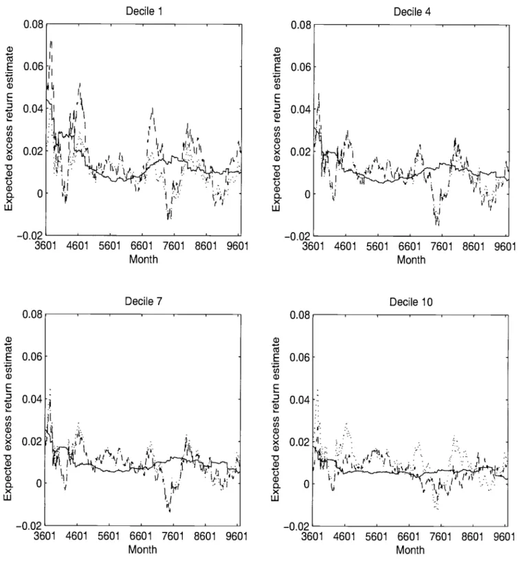
correspond to annualized maximum Sharpe ratios of 0.6 and 1.0, _{respectively.'5 Only the} restricted estimates that condition on _{are presented. As previously noted, °h is difficult} to estimate. Since the expected return vector is scaled by °h, treating °h as a free parameter leads to occasional jumps in expected return estimates in response to changes in the estimate of °h Conditioning on °h eliminates this problem.

Figures 1 and 2 present the expected return estimates for T 60 for deciles 1 (smallest

firms), 4, 7, and 10 (largest firms). Figure 1 contains the results for °h 33. The sample

mean and grand mean estimates are quite variable.16 As would be expected, the returns on small stocks are more variable than the returns on large stocks. For all deciles, the unrestricted estimates are negative in the early 40's and in the mid-70's. The restricted

estimates are much smoother. The expected return generally varies between 1-2% per month for decile 1, and between 0.5-1% per month for decile 10.17 In general, the estimates are

economically reasonable. The tendency for the unrestricted estimates to move together with

the restricted estimates appears weak. Using the information in covariances leads to expected

return estimates that are quite different from the unrestricted estimates.

Figure 2 contains the results for °h = 12. The lower value of °h implies a higher Sharpe ratio for the unobservable factor portfolio, and hence higher restricted estimates of the mean.

These restricted estimates in fact seem to be too high. For example, the expected return for deciles 1 and 4 is often near or above 2% per month. If these expected returns _seem

too high, then 0h = 12 is probably too low, and the true maximum Sharpe ratio is smaller than 1.0. Comparing the restricted and unrestricted estimates leads to the same conclusions as in Figure 1. The restricted estimates are much less variable and do not appear to move together with the unrestricted estimates.

Table 5 presents out-of-sample monthly Sharpe ratios for eight investment strategies, based on the 1936 to 1996 period as well as on two and three subperiods of equal length. Panel A presents the Sharpe ratios for three passive strategies: holding the value-weighted market index, the equal-weighted market index, and an equal-weighted portfolio of the ten deciles. The Sharpe ratios are similar across the three passive strategies. They range from

0.0784 to 0.2056, with the lowest values in the periods that include the down-market of 1973 '5RecalI that the annualized maximum Sharpe ratio equals (12/06)1/2.

'6The James-Stein estimates are obtained by shrinking the sample mean toward the grand mean, so they always lie between the two estimates.

through 1974. Panel B presents the results for portfolios constructed using the unrestricted

estimators of the mean and covariance matrix. The unrestricted estimators perform _very

poorly.18 The Sharpe ratios are low and often negative; for the overall period, they are equal

to 0.0555 and -0.0356 for estimation windows of 60 and 120 months, respectively.19

Panel C presents the results for the unrestricted mean estimator combined with the

identity matrix. Recall that using the identity covariance matrix is consistent with imposing the link between the means and covariances. In all but one case the Sharpe ratios in Panel C are higher than in Panel B, supporting the usefulness of imposing the link. Using a 60-month window, the Sharpe ratios in Panel C are quite high and in most cases exceed those of the passive portfolios. The Sharpe ratio for the overall period is 0.1728, higher than 0.1583 for the best performing passive portfolio, the equal-weighted market index. However, using a 120-month window, the results are mixed, with negative Sharpe ratios in some periods. Clearly. the unrestricted mean estimator can lead to rather unstable optimal weights, even when the covariance matrix is an identity. Moreover, as shown in Panels D and E, using the James-Stein expected return estimator does not seem to offer any improvement over the unrestricted estimator in this sample.

Panel F of Table 5 reports the results for the restricted estimators of the mean and

covariance matrix with no observed factors. Recall that the restricted covariance matrix is simply the identity. As discussed earlier, the portfolio weights are not sensitive to 0h The restricted portfolio does well, with Sharpe ratios that are always positive and comparable to (and often higher than) those of the passive portfolios. Comparison with the low Sharpe ratios for the unrestricted estimates in Panel B clearly reveals the usefulness of imposing the restrictions. The Sharpe ratios in Panel F are always higher than the corresponding ratios

in Panel B. Moreover, comparison with Panels C and E reveals that using the restricted

mean in general provides more reasonable portfolios than using either the sample mean or the James-Stein mean, even with the identity covariance matrix.

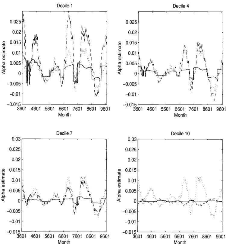
The restricted estimation approach is next applied with one observable factor portfolio, the value-weighted market index. The estimates of the mispricing c relative to the one-factor model are presented in Figures 3 and 4, for T 60. The estimates are plotted for °h = 1200

and °h 300, which corresponds to the annualized Sharpe ratios for the optimal orthogonal

'8The fact that using the unrestricted estimators to compute optimal portfolio weights often results in poorly-behaved portfolios has been documented and discussed in a number of studies, including Dickinson

(1974), Jobson and Korkie (1980), Michaud _{(1989), Best and Grauer (1991), Jorion (1991), Black and}

Litterman (1992), Green and Hollifield (1992), and Chopra and Ziemba (1993).

'9One is cautioned not to attach much significance to the magnitudes of the negative Sharpe ratios. If the mean return is negative, the magnitude of such a ratio increases as the standard deviation decreases, so that the negative ratio decreases as risk decreases.

portfolio of 0.1 and 0.2, respectively. For all deciles, the restricted mispricing estimates are much more stable than the unrestricted estimates. However, the restricted estimates

"jump" when they cross zero. Conditioning on a nonzero value of 0h_implies the existence of mispricing, so all elements of a cannot have values very close to zero. The estimated a for decile 10 is close to zero, which could be expected since this large firm decile dominates the value-weighted market index.

In portfolio selection, the value-weighted market is not included among the investable assets, since it is approximately a linear combination of the decile portfolios, and is very highly correlated with the decile containing the largest stocks. Therefore, the optimal port-folio computed here is not the orthogonal active portport-folio, but rather the tangency portport-folio of the ten assets:

1OJ (35)

where =

+

râ0 +

_{+ &I, and c}

— t'1r. The

restricted

estimates are computed assuming that there is one observable and one unobservable factor.

In addition, estimates of the mean f

andstandard deviation of the factor returns are

needed. These parameters are estimated by their sample values for the CRSP value-weighted market index from January 1926 through the last month in the estimation window.

Panel G of Table 5 reports the results for the restricted estimators of the mean and

covariance matrix with one observed factor. Since the portfolio weights are now sensitive to

°h, the results are reported for °h 1200 as well as for 9h 300. The Sharpe ratios are

much higher than for the unrestricted estimates in Panel B, except for T =60 _{and 8h}= 300

in the periods that include the 1936 to 1956 period. Comparing the Sharpe ratios from

Panels F and G leads to the somewhat counterintuitive result that one is better off not using the value-weighted market as the factor portfolio when constructing the optimal portfolio weights. This result is consistent with the importance of the link, given the empirical fact

that stock returns have one dominant factor. For the zero-factor results in Panel F, the dominant factor is missing, so there are substantial benefits from imposing the link. For

the one-factor results in Panel G, where the important factor has been largely accounted for and only relatively unimportant factors are omitted, the benefits of imposing the link are reduced. Moreover, the value-weighted market may not be a perfect proxy for the single dominant factor. The usefulness of observing the returns on the value-weighted market is further compromised given the imprecision of the estimates of its mean fi and variance

Hence, a small value for 0h implies an important missing factor and could potentially lead to extreme portfolio weights. Technically, c in equation (35) can be close to zero, which results

in extreme weights. In Panel G, this problem is present for 0h =300. Between 1936 and

1996, the absolute value of the maximum weight exceeds 100% in 146 months for T 60

and in 101 months for T 120. For °h =

1200, the absolute value of the maximum weight never exceeds 100%.

To investigate the impact of extreme weights, the results of Panel G are replicated with

one modification. The portfolio weights are adjusted so that no long or short position in

any single decile exceeds 50%. In each month for which the largest absolute weight exceeds 50%, the portfolio is modified such that that weight is reduced to 50% with the same sign. The magnitudes of the other decile weights are reduced proportionally. The value-weighted market is added to the portfolio as an extra asset so that the weights sum to one.20

The results for this modified approach are reported in Panel H. The Sharpe ratios with the modification are generally close to those without the modification, with a few exceptions. The

very low Sharpe ratios from Panel G for T 60 and °h 300 have increased substantially.

The negative ratios for the periods that include the 1936 to 1956 period are now positive and in line with the passive indexes. Clearly, the results for this period in Panel G are driven by some months with extreme weights.

5.2 Individual Stocks

The universe of 30 individual stocks is selected using the recent composition of the Dow

Jones Industrial Index. In order to be included in the sample, a stock is required to be

continuously listed on an exchange in the past 50 years.2' Among the stocks that currently constitute the Dow Jones 30 index, 22 satisfy this requirement. The additional 8 stocks that satisfy the requirement are selected from earlier Dow Jones lists.

Table 6 presents the portfolio selection results for the individual stocks. The analysis is analogous to that for the decile portfolios, with two exceptions. First, when the link between

the mean and covariance matrix is imposed, the results for T = 24 are added in order to

illustrate the approach for T < N. One advantage of the restricted approach to portfolio

selection is that there are no restrictions on the number of assets N. In contrast, using the unrestricted approach, the number of assets must be smaller than the number of time series

20The simple ad-hoc modification proposed here is only one of many ways of imposing portfolio constraints.

For example, a reasonable alternative would be to impose a restriction on the sum of squared weights.

21This criterion provides a reasonably long period for out-of-sample comparisons. The effect of survivorship

bias is unlikely to be important, since comparisons are conducted between strategies that combine the same set of stocks.

observations T, so that the sample estimate of the covariance matrix is non-singular. Second, in one-factor analysis, the factor portfolio is now included as an investable asset, since it is no longer a linear combination of the N assets. The optimal portfolio is constructed using

the result in equation (25) with the restriction =a21.

The conclusions for the individual stocks are broadly similar to those for the decile portfolios. The Sharpe ratios obtained using the unrestricted estimates (Panel B) are low and often negative. Using the identity matrix with the unrestricted mean (Panel C) leads to some improvement. Using the identity matrix with the James-Stein (Panel E) and the restricted (Panel F) mean estimates is even better. The restricted estimates from a

one-factor model (Panel G) perform quite well, except for a few cases with small °h, for the same

reason as in the previous subsection. The only strategy that yields positive and reasonable

Sharpe ratios in all subperiods and for all values of T (including T 24) is the one that uses the restricted estimates with no observed factors. Recall that this strategy uses the

identity covariance matrix with the restricted estimate of the mean, which incorporates the information from the covariances,

While both empirical examples are only illustrative, their results are promising. The restricted expected return estimates are economically reasonable and much less variable

than historical averages. The portfolio selection results show that imposing the link between the means and covariances unambiguously dominates using the estimates that do not invoke implications of an exact factor structure.

6 Conclusion.

The debate on the usefulness of factor-based pricing models has centered primarily on their ability to explain the cross section of expected returns. Some recent evidence has been

unfa-vorable toward these models. However, it is unlikely that any economic model will explain all

phenomena that can be culled from the data. This paper adopts a more positive approach to evaluating the usefulness of factor-based models. By imposing certain implications of these models in estimation of expected returns and in portfolio selection, it is shown that these models can play an important role in finance despite their apparent imperfections.

The central theme of the paper is that, given a factor structure with an unobserved factor, the vector of expected returns is directly linked to the covariance matrix of returns. Hence, the covariances provide information that can be useful in estimating the means, Simulations and empirical illustrations show that this is indeed the case. Substantially higher precision

can be obtained by employing an expected return estimator that incorporates the link.

about the covariance structure, the proposed estimators of expected returns are likely to be biased. With a long and stable time series of returns, it is possible for the noisier but

unbiased unrestricted estimates to be more precise. Nevertheless, the assumption of stability of the return distribution over very long horizons is not necessarily appropriate, so the role of the bias should not be overstated.

The link between expected returns and covariances is also important in portfolio selection.

Imposing the link is especially useful when the factors are difficult to identify precisely

and/or are unstable over time, With no observed factors, a strong form of the link leads to a

simplification in which the identity matrix is used as a covariance matrix when calculating the tangency portfolio weights.22 In all simulated cases with estimated expected returns, the true

Sharpe ratio of the tangency portfolio constructed using the identity matrix is higher than using the true covariance matrix. This result holds even when the underlying assumptions are violated. The driving force behind the result is that using the identity matrix effectively links the expected returns to the covariances, whereas using the true covariance matrix does not. The difference between using the true covariance matrix and the identity is especially large when the usual sample mean is used to estimate the expected return.

The important issue of estimation risk pioneered by Bawa, Brown, and Klein (1979) is not

addressed, for tractability reasons. When computing the optimal portfolios, the estimates of the return moments are treated as true parameters. Estimation risk can be incorporated in a Bayesian framework. With a noninformative prior, the Bayesian tangency portfolio weights correspond to the unrestricted estimator of the weight vector in (17), which alleviates the concerns about estimation risk when unrestricted estimators are used.23 Using restricted

estimators of the return moments also has a Bayesian interpretation, albeit less formal.

The restricted optimal weights are likely to be close to the weights obtained in a Bayesian

framework when the only prior information is that there is a perfect link between model mispricing and the residual covariance matrix. Conditioning on a certain value for the maximum Sharpe ratio is similar in nature to specifying a dogmatic prior belief that the

Sharpe ratio is known. Pursuing a Bayesian approach that allows the data to update a less

dogmatic prior about the link is beyond the scope of this study, but is one direction for

future research.

This paper provides economic motivation for using a simply structured covariance matrix, 221f the investable assets are sufficiently different from each other in terms of their residual variances, such as when assets from different asset classes are mixed together, a weaker form of the link that replaces an identity matrix with a more general diagonal matrix can be imposed.

23The correspondence between the Bayesian weights and the unrestricted weights follows because the mean of the Bayesian predictive density is equal to the maximum likelihood estimate of the mean, and the predictive covariance matrix is a scalar multiple of the sample covariance matrix.

such as an identity matrix, in portfolio selection. The motivation assumes that expected asset returns are driven solely by the assets' covariances with an unobserved factor. Nevertheless, an investor may believe that the assets' risk premia are not entirely risk-based, as suggested by MacKinlay (1995). In that case, a simply structured covariance matrix may serve as a

benchmark around which a Bayesian investor can center his prior beliefs about the covariance matrix. The tightness of the prior would reflect the degree of belief that the mispricing is

risk-based. This economic motivation complements the statistical motivation of Ledoit (1994) for shrinking the sample covariance matrix toward the identity matrix.

Several other issues warrant further study. The robustness of the simulation result that the identity matrix beats the true covariance matrix in portfolio selection is important. This result has strong implications for the value of efforts that seek to develop refined estimators of the covariance matrix for portfolio selection. The framework proposed here provides a natural way of allocating among many assets without imposing artificial constraints. The gains from imposing the link when the number of assets exceeds the number of time series observations deserve further investigation. Finally, empirical analysis using different sets of assets would be informative.

While there is substantial empirical evidence questioning the validity of factor-based asset

pricing models, our results suggest that casting the models aside could be premature. Even

if the pricing relation is not exact, assuming that mispricing is due to risk can serve as a

Appendix

The appendix derives the formula in (24) for the vector of optimal weights in the tangency

portfolio. From basic mean-variance analysis, this (N + 1) x 1 vector equals

XN+

(JV*_l*)_l v1

_(A.1)

where jf is the (N + 1) vector of expected excess returns with the factor portfolio as the

(N + i)8t element and V* is the (N + 1) x (N + 1) excess return covariance matrix:

V /3a

_{/3/3'a+ 3a}

v

=

_{, (A.2)}

'a a

where V 33'a + has been substituted.

V can be analytically inverted using the formula for a partitioned inverse (see Morrison

(1990), page 69):

—--'/3

=

_(A3)

_-i +

Using (A.3), f'

Lu' ftp], and substituting o —13u1. from (23), we obtain

—

>1/3IiP

= . _(A.4)

—'-1 +

+

—j3Th1c +

Returning to (A. 1), the portfolio weight vector is:

XN+ C1 , (A.5)

—/3Th1c +

References

Bawa, Vijay S., Stephen J. Brown, and Roger W. Klein, 1979, Estimation Risk and Optimal

Portfolio Choice, North Holland.

Best, M. J. and R. R. Grauer, 1991, On the sensitivity of mean-variance efficient portfolios

to changes in asset means: Some analytical and computational results, Review of

Financial Studies 4, 315—342.

Black, Fisher and Robert Litterman, 1992, Global portfolio optimization, Financial

Ana-lysts Journal, September—October 1992.

Chopra, Vijay K. and William T. Ziemba, 1993, The effect of errors in means, variances, and covariances on optimal portfolio choice, Journal of Portfolio Management, Winter

1993, 6-11.

Connor, Gregory, and Robert A. Korajczyk, 1986, "Performance measurement within the arbitrage pricing theory: A new framework for analysis," Journal of Financial Eco—

nomics 15, 373-394.

Daniel, K., and S. Titman, 1997, "Evidence on the characteristics of cross sectional variation

in stock returns," Journal of Finance 52, 133.

Dickinson, J. P., 1974, The reliability of estimation procedures in portfolio analysis, Journal of Financial and Quantitative Analysis, June, 447—462.

Fama, E. and K. French, 1993, "Common risk factors in the returns on stocks and bonds,"

Journal of Financial Economics 33, 3—56.

Gibbons, M., Ross, S. and J. Shanken, 1989, "A test of the efficiency of a given portfolio,"

Econometrica 57, 1121—1152,

Green, Richard C. and Burton Hollifield, 1992, When will mean-variance efficient portfolios be well diversified?, Journal of Finance 47, 1785—1809.

Grinblatt, Mark and Sheridan Titman, 1987, The relation between mean-variance efficiency and arbitrage pricing, Journal of Business 60, 97—112.

Huberman, Gur and Shmuel Kandel, 1987, Mean-variance spanning, Journal of Finance

42, 873—888.

Huberman, Gur, Shmuel Kandel, and Robert F. Stambaugh, 1987, Mimicking portfolios and exact arbitrage pricing, Journal of Finance 42, 1—9.

Jobson, J. D. and Bob Korkie, 1985, Some tests of linear asset pricing with multivariate

normality, Canadian Journal of Administrative Sciences 2, 114—138.

Jobson, J. D. and B. Korkie. 1980, Estimation for Markowitz efficient portfolios, Journal

of American Statistical Association 75, 544—554.

Jorion, Philippe, 1986, Bayes-Stein estimation for portfolio analysis, Journal of Financial

and Quantitative Analysis 21, 279—292.

Jorion, Philippe, 1991, Bayesian and CAPM estimators of the means: Implications for