GMM Gradient Tests for Spatial Dynamic Panel Data Models

Munich Personal RePEc Archive

GMM Gradient Tests for Spatial

Dynamic Panel Data Models

Taspinar, Suleyman and Dogan, Osman and Bera, Anil K.

2017

Online at

https://mpra.ub.uni-muenchen.de/83570/

GMM Gradient Tests for Spatial Dynamic Panel Data Models

S¨uleyman Ta¸spınar† Osman Do˘gan‡ Anil K. Bera§

2

September 29, 2016

Abstract

4

In this study, we formulate the adjusted gradient tests when the alternative model used to construct tests deviates from the true data generating process for a spatial dynamic panel data

6

model (SDPD). Following Bera et al. (2010), we introduce these adjusted gradient tests along with the standard ones within a GMM framework. These tests can be used to detect the presence

8

of (i) the contemporaneous spatial lag terms, (ii) the time lag term, and (iii) the spatial time lag terms in an higher order SDPD model. These adjusted tests have two advantages: (i)

10

their null asymptotic distribution is a central chi-squared distribution irrespective of the mis-specified alternative model, and (ii) their test statistics are computationally simple and require

12

only the ordinary least-squares (OLS) estimates from a non-spatial two-way panel data model. We investigate the finite sample size and power properties of these tests through Monte Carlo

14

studies. Our results indicates that the adjusted gradient tests have good finite sample properties.

JEL-Classification: C13, C21, C31.

16

Keywords: Spatial Dynamic Panel Data Model, SDPD, GMM, Robust LM Tests, GMM Gradient Tests, Inference.

18

∗_{This research was supported, in part, by a grant of computer time from the City University of New York High}

Per-formance Computing Center under NSF Grants CNS-0855217 and CNS-0958379. Please address all correspondence to S¨uleyman Ta¸spınar at STaspinar@qc.cuny.edu.

†_{Economics Program, Queens College, The City University of New York, United States, email:}

staspinar@qc.cuny.edu.

1

Introduction

In this study, we consider a spatial dynamic panel data model (SDPD) that includes a time lag

20

term, spatial time lag terms and contemporaneous spatial lag terms. The model is in the form of a high order spatial autoregressive model by including high orders of contemporaneous spatial

22

lag term and spatial time lag term. We formulate the GMM gradient tests, the adjusted GMM gradient tests and the C(α) test to test hypothesis about the parameters of the time lag term, the

24

spatial time lag terms and the contemporaneous spatial lag terms.

In the literature, the model specifications and estimation strategies, including the ML, GMM

26

and Bayesian methods, receive considerably more attention than the specification testing and other forms of hypothesis tests for the SDPD models. For two recent surveys, see Anselin et al. (2008)

28

and Lee and Yu (2010b). Lee and Yu (2010a, 2011, 2012a), Yu and Lee (2010), and Yu et al. (2008, 2012) consider the ML approach for dynamic spatial panel data models when both the number of

30

individuals and the number of time periods are large under various scenarios. The MLE suggested in these studies has asymptotic bias and the limiting distributions of bias corrected versions are

32

properly centered when the number of time periods grows faster than the number of individuals. Elhorst (2005), Lee and Yu (2015), and Su and Yang (2015) consider the ML approach for the

34

dynamic panel data models that have spatial autoregressive processes in the disturbance terms. Parent and LeSage (2011) introduce the Bayesian MCMC method for a panel data model that

36

accommodates dependence across space and time in the error components. Kapoor et al. (2007) extend the GMM approach of Kelejian and Prucha (2010) to a static spatial panel data model with

38

error components. Lee and Yu (2014) consider the GMM approach for an SDPD model that has high orders of contemporaneous spatial lag term and spatial time lag term.

40

To date, the focus has been on the specification testing for the cross-sectional and the static spatial panel data models (Anselin et al. 1996; Baltagi and Yang 2013; Baltagi et al. 2003, 2007;

42

Debarsy and Ertur 2010). In this study, we introduce GMM-based tests for an SDPD model that has high orders of contemporaneous spatial lag term and spatial time lag term. In particular, we

44

first consider the GMM-gredient test (or the LM test) of Newey and West (1987), which can be used to test the non-linear restrictions on the parameter vector. We also consider the C(α) test within

46

the GMM framework for the same model. While the computation of GMM-gradient test requires an estimate of the optimal restricted GMME, the computation ofC(α) test statistic requires only

48

a consistent estimate of the parameter vector. For both tests, we provide analytical justification for their asymptotic distributions within the context of our SDPD.

50

Within the ML framework, Davidson and MacKinnon (1987), Saikkonen (1989) and Bera and Yoon (1993) show that the usual LM tests are not robust to local mis-specifications in the alternative

52

models. That is, the usual LM tests have non-central chi-squared distribution when the alternative model (locally) deviates from the true data generating process. Bera et al. (2010) extent this result

54

to the GMM framework and show that the asymptotic distribution of the usual GMM-gradient test is a non-central chi-squared distribution when the alternative model deviates from the true data

56

generating process. In such a context, the usual LM and GMM-gradient tests will over reject the true null hypothesis. Therefore, Bera and Yoon (1993) and Bera et al. (2010) suggest robust (or

58

adjusted) versions that have, asymptotically, central chi-squared distributions irrespective of the local deviations of the alternative models from the true data generating process.

60

By following Bera et al. (2010), we construct various adjusted GMM-gradient tests for an SDPD model. These tests can be used to detect the presence of (i) the spatial lag terms, (ii) the time lag

62

term, and (iii) the spatial time lag terms in an SDPD model. Besides being robust to local mis-specifications, these tests are computationally simple and require only estimates from a non-spatial

64

distribution of robust tests under both the null and local alternative hypotheses. We investigate

66

the size and power properties of our suggested robust tests through a Monte Carlo simulation. The simulation results are in line with our theoretical findings and indicate that the robust tests have

68

good size and power properties.

The rest of this paper is organized in the following way. Section 2 presents the SDPD model

70

under consideration and discusses its assumptions. Section 3 lays out the details of the GMM estimation approach for the model specification. Section 4 presents the GMM gradient tests, the

72

adjusted GMM gradient tests and theC(α) test. Section 5 lays out the details of the Monte Carlo design and presents the results. Section 6 closes with concluding remarks. Some of the technical

74

derivations are relegated to an appendix.

2

The Model Specification and Assumptions

76

Using the standard notation, an SDPD model with both individual and time fixed effects is stated as

Ynt = p

X

j=1

λj0WnjYnt+γ0Yn,t−1+

p

X

j=1

ρj0WnjYn,t−1+Xntβ0+cn0+αt0ln+Vnt (2.1)

for t= 1,2, . . . , T, where Ynt = (y1t, y2t, . . . , ynt)

′

is the n_×1 vector of a dependent variable, Xn

is the n_×kx matrix of non-stochastic exogenous variables with a matching parameter vector β0,

78

and Vnt = (v1t, . . . , vnt)

′

is the n_×1 vector of disturbances (or innovations). The spatial lags of the dependent variable at time t and t₋1 are, respectively, denoted by WnjYnt and WnjYn,t−1

80

for j = 1, . . . , p. Here, Wnjs are the n× n spatial weight matrices of known constants with

zero diagonal elements, λ0 = (λ10, . . . , λp0)

′

and ρ0 = (ρ10, . . . , ρp0)

′

are the spatial autoregressive

82

parameters. The individual fixed effects are denoted by cn0 = (c1,0, . . . , cn,0)

′

and the time fixed effect is denoted by αt0ln, where ln is the n×1 vectors of ones. For the identification of fixed

84

effects, Lee and Yu (2014) impose the normalization l_n′cn0 = 0. For the estimation of the model,

we assume that Yn0 is observable. Let Θ be the parameter space of the model. In order to

86

distinguish the true parameter vector from other possible values in Θ, we state the model with the true parameter vector θ0 = λ

′

0, δ

′

0

′

, where δ0 = γ0, ρ

′

0, β

′

0

′

. Furthermore, for notational

88

simplicity we let Sn(λ) = In−Ppj=1λjWnj, Sn = Sn(λ0), An = Sn−1 γ0In +Ppj=1ρjWnj,

Gnj(λ) =WnjSn−1(λ),Gnj =Gnj(λ0) and N =n(T−1).

90

To avoid the incidental parameter problem, the model is transformed to wipe out the fixed effects. The individual effects can be eliminated from the model by employing the or-thonormal eigenvector matrix FT,T−1,√1_TlT of JT = IT − _T1lTl

′

T

, where FT,T−1 is the

T _×(T ₋1) eigenvectors matrix corresponding to the eigenvalue one and lT is the T ×1

vec-tor of ones corresponding to the eigenvalue zero.1 This orthonormal transformation can be applied by writing the model in an n _× T system. Hence, the dependent variable is trans-formed as Yn1, Yn2, . . . , YnT×FT,T−1 =Yn∗1, Yn∗2, . . . , Yn,T∗ −1

, and alsoYn0, Yn1, . . . , Yn,T−1×

FT,T−1 =

Y_n(₀∗,−1), Y_n(₁∗,−1), . . . , Y_n,T(∗,−₋1)₂. Similarly, Xnj,1, Xnj,2, . . . , Xnj,T

× FT,T−1 =

X_nj,∗ ₁, X_nj,∗ ₂, . . . , X_nj,T∗ ₋₁forj = 1, . . . , kx,Vn1, Vn2, . . . , VnT×FT,T−1 =Vn∗1, Vn∗2, . . . , Vn,T∗ −1

, and α10, α20, . . . , αT0×FT,T−1 =α∗10, α∗20, . . . , α∗T−1,0

. Since the column of FT,T−1,√1_TlTare

orthonormal, we have [cn0,cn0, . . . ,cn0]×FT,T−1 = 0n×(T−1). Thus, the transformed model does

1_{This orthonormal matrix has the following properties (i) JTFT ,T}

−1 = FT ,T−1 and JTlT = 0T×1, (ii)

FT ,T′ −1FT ,T−1=IT−1 andF

′

T ,T−1lT = 0(T−1)×1, (iii)FT ,T−1F

′

T ,T−1+T1lTl ′

T =IT and (iv)FT ,T−1F

′

not include the individual fixed effects and can be written as

Y_nt∗ =

p

X

j=1

λj0WnjYnt∗ +γ0Yn,t(∗,−−11)+

p

X

j=1

ρj0WnjYn,t(∗,−−11)+Xnt∗ β0+α∗t0ln+Vnt∗ (2.2)

for t = 1, . . . , T ₋1. We consider the forward orthogonal difference (FOD) transformation for the orthonormal transformation. Hence, the terms in (2.2) can be explicitly stated as V∗

nt = T−t

T−t+1

1/2

Vnt− _T1_−tPTh=t+1Vnh,Yn,t(∗,−−11) = TT−−t+1t

1/2

Yn,t−1−_T1_−tPhT=−t1Ynh, and the others

terms are defined similarly. Let V∗_n,T−1 = V_n∗₁′, . . . , V_n,T∗′ ₋₁′. Then, Var V_n,T∗ ₋₁ = F_T,T′ _−1⊗ InE VnTV

′

nT

FT,T−1 ⊗In = σ20IN by Assumption 1. The transformed model in (2.2) still

includes the time fixed effect α∗_t0ln, which can be eliminated by pre-multiplying the model with

Jn=In−1_nlnl

′

n. The resulting model is free of the fixed effects, fort= 1, . . . , T −1,

JnYnt∗ = p

X

j=1

λj0JnWnjYnt∗ +γ0JnYn,t(∗,−−11)+

p

X

j=1

ρj0JnWnjYn,t(∗,−−11)+JnXnt∗ β0+JnVnt∗. (2.3)

The consistency and asymptotic normality of the GMME ofθ0 are established under Assumptions 1

through 5.2

92

Assumption 1. — The innovations vits are independently and identically distributed across i

and t, and satisfy E (vit) = 0, E vit2

=σ2

0, and E|vit|4+η <∞ for someη >0 for all iandt.

94

Assumption 2. — The spatial weight matrix Wnjs is uniformly bounded in row and column

sums in absolute value for j = 1, . . . , p, and _kPp_j=1λj0Wnjk∞ <1. Moreover, Sn−1(λ) exists and

96

is uniformly bounded in row and column sums in absolute value for all values of λ in a compact parameter space.

98

Assumption 3. — Letη >0 be a real number. Assume thatXnt,cn0, andα_t0are non-stochastic

terms satisfying (i) sup_{n,T nT}1 PT_t=1Pn_i=1|xit,l|2+η <∞ forl = 1, . . . , kx, where xit,l is the (i, t)th

100

element of thelthcolumn, (ii) limn→∞ n(T1−1)

PT−1

t=1 Xnt∗ JnXnt∗ exists and is non-singular, and (iii)

sup_{T T}1 PT_t=1|αt0|2+η <∞ and supnn1

Pn i=1|ci0|

2+η

<_∞.

102

Assumption 4. — The DGP for the initial observations is Yn0 =

Ph∗

h=0AhnSn−1(cn0+Xn,−hβ0+α−h,0ln+Vn,−h), whereh∗ could be finite or infinite.

104

Assumption 5. — The elements of P∞_h=0abs Ah_n are uniformly bounded in row and column sums in absolute value, where [abs (An)]ij =|An,ij|

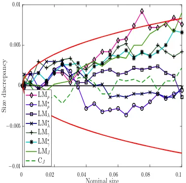
106

3

The GMM Estimation Approach

In this section, we summarize the GMM estimation approach for (2.3) under both largeT and finite

T scenarios. The model in (2.3) indicates that IVs are needed forWnjYnt∗,Y

(∗,−1)

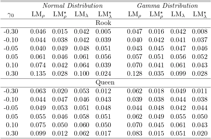
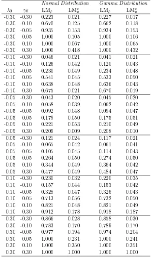
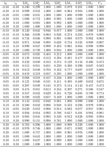
n,t−1 , andWnjYn,t(∗,−−11)

for each t. Before, we introduce the set of moment functions, it will be convenient to introduce some further notations. LetZ_nt∗ =Y_n,t(∗,₋−₁1), Wn1Y_n,t(∗,₋−₁1), . . . , WnpY_n,t(∗,₋−₁1), Xnt∗

,Jn,T−1 =IT−1⊗Jn,

andV_n,T∗ ₋₁(θ) = V_n∗₁′(θ), . . . , V_n,T∗′ ₋₁(θ)′ whereV_nt∗(θ) =Snt(λ)Ynt∗ −Znt∗ δ−α∗tln. We consider the

following (m+q)_×1 vector of moment functions

gnT(θ) =

       

V∗_n,T′ ₋₁(θ)Jn,T−1Pn1,T−1Jn,T−1V∗n,T−1(θ)

V∗_n,T′ ₋₁(θ)Jn,T−1Pn2,T−1Jn,T−1V∗_n,T−1(θ)

.. .

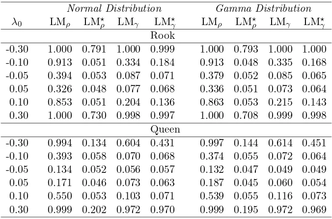
V_n,T∗′ ₋₁(θ)Jn,T−1Pnm,T−1Jn,T−1Vn,T∗ −1(θ)

Q′_n,T−1Jn,T−1V∗n,T−1(θ)

       

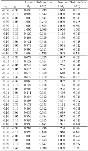
. (3.1)

In (3.1), Pnj,T−1 = IT−1 ⊗Pnj, where Pnj is the n ×n quadratic moment matrix satisfying

108

tr (PnjJn) = 0 forj= 1, . . . , m, andQn,T−1 = Q

′

n1, . . . , Q

′

n,T−1

′

is theN_×q liner IV matrix such thatq_≥kx+2p+1. Under Assumptions 1-4, it can be shown that _N1 ∂gnT_∂θ(′θ0) =DnT+RnT+O √1_nT,

110

whereDnT isO(1) andRnT isO _T1

.3

Let vecD(·) be the operator that creates a column vector from the diagonal elements of an input

square matrix. For the optimal GMM estimation, we need to calculate the covariance matrix of moment functions E g_nT′ (θ0)gnT (θ0), which can be approximated by

ΣnT =σ40 1

N∆nm,T 0m×q

0q×m _σ12 0

1

NQ

′

n,T−1Jn,T−1Qn,T−1

!

(3.2)

+ 1

N

µ4−3σ04

ω_nm,T′ ωnm,T 0m×q

0q×m 0q×m

,

where ωnm,T = vecD(Jn,T−1Pn1,T−1Jn,T−1), . . . ,vecD(Jn,T−1Pnm,T−1Jn,T−1),

112

∆nm,T = vec(Jn,T−1P

′

n1,T−1Jn,T−1), . . . ,vec(Jn,T−1P

′

nm,T−1Jn,T−1)

′

×

vec(Jn,T−1Psn1,T−1Jn,T−1), . . . ,vec(Jn,T−1Psnm,T−1Jn,T−1), where Asn = An + A

′

n for any

114

square matrix An.

Let ΣbnT be a consistent estimate of ΣnT. Then, the optimal GMME is defined by

b

θnT = argminθ∈Θg

′

nT(θ)Σb−nT1gnT(θ) (3.3)

Under Assumptions 1 - 5, Lee and Yu (2014) show that when both T and ntend to infinity4_:

√

N θbnT −θ0−→d N

0,hplim_n,T→∞D_nT′ Σ−_nT1DnT

i−1

. (3.4)

When T is finite, the GMME in (3.4) is still consistent and unbiased but its limiting covariance

116

matrix is different, since the additional termRnT =O _T1does not vanish. Hence, whenT is finite,

the asymptotic covariance matrix of√N θbnT−θ0is given byplimn→∞ DnT+RnT

′

Σ−_nT1 DnT+

118

RnT−1.

3_{The explicit forms forDnT andRnT are not required for our testing results, hence they are not given here. For}

these terms, see Lee and Yu (2014).

4 _{Lee and Yu (2014) state the identification conditions. Here, we simply assume that the parameter vector is}

4

The GMM Gradient Tests

In this section, we consider various version of the gradient test (LM test). Let r:R2p+kx+1 _→Rkr

be a twice continuously differentiable function, and assume that R(θ) = ∂r(θ)

∂θ′ has rank kr.

122

Consider the implicit restrictions denoted by the null hypothesis H0 : r(θ0) = 0. Define

b

θnT,r = argmax_{θ:r(θ)=0}Qn, where Qn =g

′

nT(θ)Σb−nT1gnT(θ), as a restricted (or constrained)

opti-124

mal GMME.

In order to give a general argument, consider the following partition of θ = β′, ψ′, φ′′, where ψ and φ are, respectively, kψ ×1 and kφ × 1 vectors such that kψ + kφ = 2p + 1.

In the context of our model, ψ and φ can be any combinations of the remaining parameters, namely, λ′, γ, ρ′′. Let Ga = _N1 ∂gnT_∂a′(θ), Ca = G

′

a(θ)Σb−nT1gnT(θ), where a ∈ {β, ψ, φ} and

g_nT = _N1gnT. Define G(θ) = Gβ(θ), Gψ(θ), Gφ(θ), and C(θ) = C

′

β(θ), C

′

ψ(θ), C

′

φ(θ)

′

, and B(θ) = G′(θ)Σb_nT−1G(θ). Finally, let _Ga = plimn,T→∞N1

∂gnT(θ0)

∂a′ for a ∈ {β, ψ, φ}. Define

G = _Gβ,Gψ,Gφ

and _H = plim_n,T→∞ DnT +Rnt

′

b

Σ−_nT1 DnT +Rnt. We consider the following

partition of B(θ) and _H:

B(θ) =  

Bβ(θ) Bβψ(θ) Bβφ(θ)

Bψβ(θ) Bψ(θ) Bψφ(θ)

Bφβ(θ) Bφψ(θ) Bφ(θ)



, _H= 

_HHψββ HHβψψ HHψφβφ

Hφβ Hφψ Hφ



. (4.1)

With the notation introduced, the standard LM test statistic for H0 :r(θ0) = 0 is defined in

the following way (Newey and West 1987):

LM =N C′ bθnT,rB−1 bθnT,rC bθnT,r. (4.2)

A similar test is the C(α) test.5 This test is designed to deal with the nuisance parameters when testing the parameter of main interest (Bera and Bilias 2001). Lee and Yu (2012b) investigate the finite sample properties of this test for a cross-sectional autoregressive model. Their simula-tion results indicate that this test can be useful to test the possible presence of spatial correlasimula-tion through a spatial lag in the spatial autoregressive (SAR) model. Here, we provide a general de-scription of this test within the context of our SDPD model. By the implicit function theorem, the set of kr restrictions on θ0 can also be stated as h(ξ0) = θ0, where h : Rq → R2p+kx+1

is continuously differentiable, ξ0 contains the free parameters, and q = 2p+kx+ 1−kr. Define

bξ_nT = argmin_φg_nT′ (h(ξ))Σb_nT−1gnT (h(ξ)). Then, we havebθnT,r =h bξnT

. Let ˜ξnT be a consistent

es-timate ofξ0. DenoteGξ(θ) = _N1 ∂g_∂ξnT′(θ),Cξ(θ) =G

′

ξ(θ)Σb−nT1gnT(θ), andBξ(θ) =G

′

ξ(θ)Σb−nT1Gξ(θ).

Following the formulation suggested by Breusch and Pagan (1980), we state theC(α) test statistic in the following way

C(α) =NC′ h( ˜ξnT)B−1 h( ˜ξnT)C h( ˜φnT)− C

′

ξ h( ˜ξnT)B_ξ−1 h( ˜ξnT)Cξ h( ˜ξnT). (4.3)

In (4.3), it is important to note that ˜ξnT can be any consistent estimator. In the case where ˜ξnT is an

126

optimal GMME, the C(α) statistic reduces to LM statistic, since Cξ

h( ˜ξnT)

= 0 by definition.6 The asymptotic distributions of C(α) andLM are given in the following proposition.

128

5_{Breusch and Pagan (1980) call this test the pseudo-LM test, since its test statistic is very similar to the form of}

the LM statistic.

6_{In the context of ML estimation, theC(α) statistic reduces to the LM statistic when the restricted MLE is used.}

Proposition 1. — Given our stated assumptions, we have the following results under H0 :

r(θ0) = 0:

LM _−→d χ2_kr, and C(α)_−→d χ2_kr. (4.4)

Proof. See Section C.1.

Next, we consider the following joint null hypothesis:

H0:λ0= 0, ρ0 = 0, γ0 = 0, HA: At least one parameter is not equal to zero. (4.5)

Under the joint null hypothesis, the model reduces to a two-way non-spatial panel data model which can be estimated by an OLSE (for the estimation of two-way models, see Baltagi (2008) and Hsiao (2014)). The joint null hypothesis can be tested either by LM orC(α). Let ˜θnT be a constrained

optimal GMME under the joint null hypothesis, and letbθnT be any other consistent estimator of

θ0 under the null hypothesis. As stated in Newey and West (1987), the LM test statistic should be

formulated with the optimal constrained GMME. Letϑ= λ′, ρ′, γ′. Then, the LM test statistic for the joint null hypothesis can be expressed as

LMJ θ˜nT=N C

′

J θ˜nTBϑ·β

˜

θnT −1CJ θ˜nT, (4.6)

where C_J′ θ˜nT = C

′

λ θ˜nT

, C_ρ′ θ˜nT, C

′

γ θ˜nT

′

, Bϑ·β θ˜nT = Bϑ θ˜nT −

Bϑβ θ˜nTB_β−1 θ˜nTBβϑ θ˜nT, Bϑβ θ˜nT = B

′

βϑ θ˜nT

= B_λβ′ θ˜nT, B

′

ρβ θ˜nT

, B_γβ′ θ˜nT

′

, and

Bϑ θ˜nT=

 

Bλ θ˜nT Bλρ θ˜nT Bλγ θ˜nT

Bρλ θ˜nT Bρ θ˜nT Bργ θ˜nT

Bγλ θ˜nT

Bγρ θ˜nT

Bγ θ˜nT



. (4.7)

Similarly, the consistent estimator bθnT can be used to formulate the following C(α) test for the

joint null hypothesis:

CJ(α) =NC

′

bθnTB−1 bθnTC bθnT−C

′

β bθnTB_β−1 θbnTCβ bθnT. (4.8)

The properties of the LM test can be investigated under a sequence of local alternatives (Bera and Bilias 2001; Bera and Yoon 1993; Bera et al. 2010; Davidson and MacKinnon 1987; Saikkonen 1989). Bera and Yoon (1993) and Bera et al. (2010) suggest robust LM tests when the alternative model is misspecified. We consider similar robust LM tests within the context of our model. In order to give a general result, we consider the LM test forH₀ψ :ψ0 = 0 when H0φ :φ0 = 0, which

can be stated as

LMψ =N C

′

ψ θ˜nTBψ·β θ˜nT−1Cψ θ˜nT, (4.9)

where Bψ·β θ˜nT

= Bψ θ˜nT

− Bψβ θ˜nT

B_β−1 θ˜nT

Bβψ θ˜nT

. We investigate the asymptotic distribution of LMψ under the sequences of local alternatives H_Aψ : ψ = ψ0 +δψ/

√

N, and

H_Aφ : φ = φ0 + δφ/

√

N, where ψ₀′, φ′₀′ is the vector of hypothesized values under the null, and δψ and δφ are bounded vectors. The distribution of (4.9), under HAψ and H

φ

A, can be

θ∗ = β₀′, ψ′₀+δ_ψ′/√N , φ′₀+δ_φ′/√N′. These expansions can be written as

√

N Cψ θ˜nT=

√

N Cψ θ∗−G

′

ψ(θ∗)Σb−nT1Gψ θ

δψ−G

′

ψ(θ∗)Σb−nT1Gφ θ

δφ (4.10)

+√N G′_ψ(θ∗)Σb−_nT1Gβ θ

_˜

βnT −β0+op(1),

√

N Cβ θ˜nT=

√

N Cβ(θ∗)−G

′

β(θ∗)Σb−nT1Gψ θ

δψ−G

′

β(θ∗)Σb−nT1Gφ θ

δφ (4.11)

+√N G′_β(θ∗)Σb−_nT1Gβ θ

_˜

βnT −β0+op(1),

where θlies between ˜θnT and θ∗. Note that θ∗ =θ0+op(1) impliesθ=θ0+op(1). By Lemma 1,

we haveB(θ∗_{) =H+op(1), andG}′

(θ∗_{)ΣbnT =G}′

ΣnT+op(1). Then, from (4.10) and (4.11), we get

the following fundamental result:

√

N Cψ θ˜nT=G

′

ψΣ−nT1 − HψβH−β1G

′

βΣ−nT1

1

√

N gnT(θ0) (4.12)

−Hψ− HψβH_β−1Hβψδψ−Hψφ− HψβH−_β1Hβφδφ+op(1).

By Lemma 1, we have √1

NgnT(θ0) d

−

→ N 0,plim_n→∞ΣnT, and thus (4.12) implies that

130

√

N Cψ θ˜nT −→d N − Hψ·βδψ − Hψφ·βδφ,Hψ·β, where Hψ·β = Hψ − HψβH−_β1Hβψ, and

Hψφ·β = Hψφ − HψβH_β−1Hβφ. Hence, LMψ θ˜nT −→d χ2_kψ(ϑ1) under H_Aψ and H_Aφ, where

132

ϑ1 = δ

′

ψHψ·βδψ +δ

′

ψHψφ·βδφ +δ

′

φH

′

ψφ·βδψ +δ

′

φH

′

ψφ·βH−ψ·1βHψφ·βδφ is the non-centrality

parame-ter.7 _{We provide the distributional results for LM}

ψ θ˜nT and its robust version in the following

134

proposition.

Proposition 2. — Given our stated assumptions, the following results hold.

136

1. UnderH_Aψ and H_Aφ, we have

LMψ θ˜nT−→d χ2kψ(ϑ1), (4.13)

whereϑ1 =δ

′

ψHψ·βδψ+δ

′

ψHψφ·βδφ+δ

′

φH

′

ψφ·βδψ+δ

′

φH

′

ψφ·βH−ψ·1βHψφ·βδφ.

2. UnderH_Aψ and H₀φ, we have

LMψ θ˜nT

d

−

→χ2_kψ(ϑ2), (4.14)

whereϑ2 =δ

′

ψHψ·βδψ.

138

3. UnderH₀ψ and H_Aφ, we have

LMψ θ˜nT−→d χ2kψ(ϑ3), (4.15)

whereϑ3 =δ

′

φH

′

ψφ·βH−ψ·1βHψφ·βδφ.

4. Let C⋆′

ψ θ˜nT

= Cψ θ˜nT −Bψφ·β θ˜nTB_φ−_·1_β θ˜nTCφ θ˜nT be the adjusted pseudo-score,

whereBψφ·β θ˜nT=Bψφ θ˜nT−Bψβ θ˜nTBβ−1 θ˜nTBβφ θ˜nT, and Bφ·β θ˜nT=Bφ θ˜nT−

Bφβ θ˜nTB_β−1 θ˜nTBβφ θ˜nT. Under H0ψ and irrespective of whether H0φ or HAφ holds, we

have

LM_ψ⋆ θ˜nT=N C⋆

′

ψ θ˜nTBψ·β θ˜nT−Bψφ·β θ˜nTB_φ−_·1_β θ˜nTB

′

ψφ·β θ˜nT−1Cψ⋆ θ˜nT d

−

→χ2_kψ. (4.16)

5. UnderH_Aψ and H₀φ, we have

LM_ψ⋆ θ˜nT−→d χ2kψ(ϑ4), (4.17)

whereϑ4 =δ

′

ψ Hψ·β− Hψφ·βH−φ·1βH

′

ψφ·β

δψ.

140

Proof. See Section C.2.

There are three important observations regarding to the results presented in Proposition 2.

142

First, the one directional test has a non-central chi-square distribution when the alternative model is misspecified, i.e., when the alternative model includes φ0. The non-centrality parameter is

144

ϑ3 = δ

′

φH

′

ψφ·βH−ψ·1βHψφ·βδφ, which would be zero if and only if Hψφ·β = 0. Second, the robust

test LM_ψ⋆ θ˜nT has a central chi-square distribution even when the alternative model is locally

146

misspecified. Finally, LM⋆

ψ θ˜nT has less asymptotic power than LMψ θ˜nT, since ϑ2 −ϑ4 ≥ 0

underH_Aψ and H₀φ.

148

Proposition 2 provides a template that can be used to determine the test statistics for the following hypotheses:

150

1. The null hypothesis for the contemporaneous spatial lag terms: Hλ

0 :λ0 = 0 in the presence

of ρ0 andγ0.

152

2. The null hypothesis for the spatial lag terms at time t₋1: H₀ρ:ρ0= 0 in the presence ofλ0

and γ0.

154

3. The null hypothesis for the time lag term: H₀γ :γ0= 0 in the presence ofλ0 and ρ0.

In the following, we provide the test statistic for each hypothesis and leave the detailed derivations to Appendix B. We start with Hλ

0 :λ0 = 0. In the context of this hypothesis, φ= ρ

′

, γ′. Then, the one directional test can be written as

LMλ θ˜nT=N C

′

λ θ˜nTBλ·β θ˜nT−1Cλ θ˜nT, (4.18)

where Bλ·β θ˜nT

= Bλ θ˜nT

−Bλβ θ˜nT

B_β−1 θ˜nT

Bβλ θ˜nT

. Then, LMλ θ˜nT

d

−

→ χ2_p(ϑ2)

un-der H_Aλ and H₀φ; and LMλ θ˜nT →−d χ2p(ϑ3) under H0λ and H

φ

A, where ϑ2 = δ

′

λHλ·βδλ and

ϑ3=δ

′

φH

′

λφ·βH−λ·1βHλφ·βδφ. The robust version is stated as

LM_λ⋆ θ˜nT=N C⋆

′

λ θ˜nTBλ·β θ˜nT−Bλφ·β θ˜nTB_φ−_·1_β θ˜nTB

′

λφ·β θ˜nT−1Cλ⋆ θ˜nT, (4.19)

where C⋆ λ θ˜nT

= Cλ θ˜nT−Bλφ·β θ˜nTB−_φ·1_β θ˜nTCφ θ˜nT is the adjusted score. Irrespective

156

of whether H₀φ or H_Aφ holds, LM_λ⋆ θ˜nT has an asymptotic χ2p distribution under H0λ by

Propo-sition 2. Finally, under H_Aλ and H₀φ, we have LM_λ⋆ θ˜nT

d

−

→ χ2_p(ϑ4), where ϑ4 = δ

′

λ Hλ·β −

158

Hλφ·βH−φ·1βH

′

λφ·β

Next, we consider H₀ρ : ρ0 = 0. In the context of this hypothesis, φ = λ

′

, γ′. The one directional test can be written as

LMρ θ˜nT=N C

′

ρ θ˜nTBρ·β θ˜nT−1Cρ θ˜nT, (4.20)

where Bρ·β θ˜nT

= Bρ θ˜nT

− Bρβ θ˜nT

B_β−1 θ˜nT

Bβρ θ˜nT

. Proposition 2 implies that

LMρ θ˜nT −→d χ2p(ϑ2) under H_Aρ and H0φ; and LMρ θ˜nT −→d χ2p(ϑ3) under H0ρ and H

φ

A, where

ϑ2=δ

′

ρHρ·βδρand ϑ3 =δ

′

φH

′

ρφ·βH−ρ·1βHρφ·βδφ. The robust version of LMρ θ˜nT

is stated as

LM_ρ⋆ θ˜nT=N C⋆

′

ρ θ˜nTBρ·β θ˜nT−Bρφ·β θ˜nTB_φ−_·1_β θ˜nTB

′

ρφ·β θ˜nT−1Cρ⋆ θ˜nT, (4.21)

where C⋆

ρ θ˜nT =Cρ θ˜nT−Bρφ·β θ˜nTB−_φ·1_β θ˜nTCφ θ˜nT. The asymptotic null distribution of

160

LM_ρ⋆ θ˜nT

is χ2_p, irrespective of whether H₀φ or H_Aφ holds. Finally, under H_Aρ and H₀φ, we have

LM_ρ⋆ θ˜nT−→d χ2p(ϑ4), where ϑ4 =δ

′

ρ Hρ·β− Hρφ·βH−φ·1βH

′

ρφ·β

δρ.

162

Finally, we consider H₀γ :γ0 = 0. Here, we have φ= λ

′

, ρ′′. The one directional test can be written as

LMγ θ˜nT=N C

′

γ θ˜nTBγ·β θ˜nT−1Cγ θ˜nT, (4.22)

where Bγ·β θ˜nT = Bγ θ˜nT−Bγβ θ˜nTBβ−1 θ˜nTBβγ θ˜nT. Then, LMγ θ˜nT −→d χ21(ϑ2)

un-der H_Aγ and H₀φ; and LMγ θ˜nT −→d χ21(ϑ3) under H0γ and HAφ, where ϑ2 = δ

′

γHγ·βδγ and

ϑ3=δ

′

φH

′

γφ·βH−γ·1βHγφ·βδφ. The robust version is stated as

LM_γ⋆ θ˜nT=N C⋆

′

γ θ˜nTBγ·β θ˜nT−Bγφ·β θ˜nTB−_φ·1_β θ˜nTB

′

γφ·β θ˜nT−1Cγ⋆ θ˜nT, (4.23)

where C⋆

γ θ˜nT =Cγ θ˜nT−Bγφ·β θ˜nTB_φ−_·1_β θ˜nTCφ θ˜nT. The asymptotic null distribution of

LM_γ⋆ θ˜nT is χ21, irrespective of whether H0φ or H

φ

A holds. Finally, under H γ

A and H φ

0, we have

164

LM_γ⋆ θ˜nT−→d χ21(ϑ4), where ϑ4 =δ

′

γ Hγ·β − Hγφ·βHφ−·1βH

′

γφ·β

δγ.

5

Monte Carlo Simulation

166

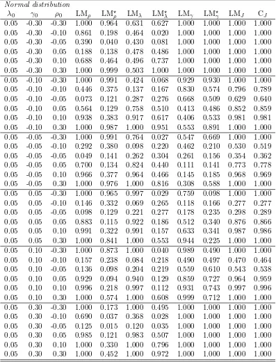
In this section, we describe the details of Monte Carlo design for our analysis. Our design is based on Lee and Yu (2014) and Yang (2015). For the model in (2.1), we will focus on the case where

p= 1:

Ynt =λ0WnYnt+γ0Yn,t−1+ρ0WnYn,t−1+Xntβ0+cn0+αt0ln+Vnt, (5.1)

fort= 1,2, . . . , T. We generate the weights matrix according to (i) Rook contiguity and (ii) Queen contiguity. Thenspatial units are randomly permuted and allocated into a lattice ofk_×msquares,

168

wherem_≥n. In the Rook contiguity, wij,n= 1 if the spatial unitj is in a square that is adjacent

(left/right/above or below) to the square of the spatial uniti. In the Queen contiguity,wij,n= 1 if

170

the spatial unitj is in a square that is adjacent to or shares a corner with the square of the spatial uniti. In both cases, Wn is row normalized.

172

We allow for two exogenous regressors. The first one is generated asX1,nt= Ψn+ 0.01t ln+Unt,

whereUnt= 0.5Un,t−1+εnt+0.5εn,t−1andεnt∼N(0n×1,2In). Furthermore, Ψn= Υn+1/(T+m+

1)PT_t=−mεnt, where Υn∼N(0n×1, In) and m= 20. Then, Xnt = X1,nt, WnX2,nt whereX2,nt∼

N(0n×1, In). We set β0 = (1.2,0.6). For the individual effects, we let cn0 = (1/T)PT_t=1X1,nt,

176

and draw αt0 from N(0,1). For the error term Vi,nt, we specify two cases: (i) Vi,nt ∼N(0,1) and

(ii) Vi,nt ∼Gamma(1,1)−1. The data generating process has 21 +T periods and the last T + 1

178

periods are used for estimation. For the sample size, we use the following nand T combinations: (n, T) =_{(100,10),(20,200)_}.8

180

Under the null model (i.e., λ0 =γ0 =ρ0 = 0), (5.1) reduces to a two-way error model (2WE).

We can employ seven different specifications for the alternative model. We choose to focus on

182

the following four specifications as they are more common in empirical applications. The first specification is a dynamic panel data model with no spatial effects (DPD), i.e., whenλ0 =ρ0 = 0

184

and γ0 6= 0 in (5.1). The second specification is a spatial static panel model (SSPD), i.e., when

λ0 6= 0 and ρ0 = γ0 = 0 in (5.1). The third specification is a spatial dynamic panel data model

186

with no spatial-time lag (SDPDW), i.e., when ρ0 = 0, λ0 6= 0 and γ0 6= 0 in (5.1). The final

specification for the alternative modes is the spatial dynamic panel data model (SDPD), i.e., when

188

ρ0 6= 0, λ0 6= 0 andγ0 6= 0 in (5.1). Note that the first three alternative models can be considered

as the null models for the one-directional tests and their robust counterparts in the following

190

way: (i) the DPD model for LMρ, LM⋆ρ, LMλ and LM⋆λ; (ii) the SSP model for LMρ, LM⋆ρ, LMγ

and LM⋆_γ; (iii) the SDPDW model for LMρ and LM⋆ρ. We let λ0, γ0 and ρ0 take values from

192

{−0.3,₋0.1, ,₋0.05,0.05,0.1,0.3_} for the alternative models. Hence, the DPD, SSPD, SDPDW and SDPD specifications yield respectively 6, 6, 16 and 216 combinations. Resampling is carried

194

out for 5,000 times.

Table 1 summarizes the null hypotheses and the respective test statistics along with the source

196

of misspecification in each hypothesis considered in the Monte Carlo study. For example, the source of misspecification for H0 :λ0 = 0 is the presence of ρ0 and γ0 in the alternative model. All test

198

statistics presented in Table 1 are computed by the estimates from the 2WE model. For the test statistics, we also need to specify the set of moment functions. The set of linear moments consists

200

of Qnt = Yn,t−1, WnYn,t−1, Wn2Yn,t−1, Xn,t∗ , WnXn,t∗ , Wn2Xn,t∗

for t = 1,2, . . . , T ₋1. For the quadratic moments, we employPn1 =Wn−tr(WnJn)/(n−1)Jn and Pn2 =Wn2−tr(Wn2Jn)/(n−

202

1)Jn. Note that we do not consider the conditional tests that require a restricted GMME (see

Proposition 1) for the computation of the test statistics. Here our aim is to compare the performance

204

of the robust tests with their non-robust counterparts once the estimates of the simple 2WE model are available.

206

5.1 Results on Size Properties

A P value discrepancy plots is generated from the empirical distribution function (edf) ofpvalues.

208

To see how, letτ denote a test statistic, andτj forj= 1, . . . ,Rbe theRrealizations ofτ generated

in a Monte Carlo experiment. Let F(x) denote the cumulative distribution function (cdf) of the

210

asymptotic distribution ofτ evaluated at the levelx. Then, thepvalue associated with τj, denoted

by p(τj), is given by p(τj) = 1−F(τj). An estimate of the cdf of p(τ) can be constructed simply

212

from the edf of p(τj). Consider a sequence of levels denoted by {xi} for i = 1, . . . , m from the

interval (0,1). Then, an estimate of the cdf of p(τ) is given by Fb(xi) =P_jR₌₁1 p(τj)≤xi/R.9

214

The P value discrepancy plot is created by plotting Fb(xi)−xi against xi under the

assump-tion that the true data generating process is characterized by the null hypothesis. To asses the

216

8_{For the sake of brevity, we only provide estimation results for (n, T) = (100,10).}

9_{We choose the following sequence and focus on the levels smaller than or equal to 0.1:{xi}}m

i=1={0.001 : 0.001 :

Table 1: Summary of test statistics

Null hypothesis Parameter Test statistic

Spatial time lag: ρ0 Time lag: γ0

H0:λ0= 0 Set to zero Set to zero LMλin (4.18)

H0:λ0= 0 Unrestricted, not estimated Unrestricted, not estimated LM⋆λin (4.19)

Contemporaneous spatial lag: λ0 Time lag: γ0

H0:ρ0= 0 Set to zero Set to zero LMρin (4.20)

H0:ρ0= 0 Unrestricted, not estimated Unrestricted, not estimated LM⋆ρin (4.21)

Contemporaneous spatial lag: λ0 Spatial time lag: ρ0

H0:γ0= 0 Set to zero Set to zero LMγin (4.22)

H0:γ0= 0 Unrestricted, not estimated Unrestricted, not estimated LM⋆γin (4.23)

H0:λ0= 0, ρ0= 0, γ0 = 0 – – LMJ in (4.6)

H0:λ0= 0, ρ0= 0, γ0 = 0 – – CJ in (4.8)

significance of discrepancies in a P value discrepancy plot, we construct a point-wise 95% confi-dence interval for a nominal size by using a normal approximation to the binomial distribution

218

(Anselin et al. 1996). Let α denote the nominal size at which the test is carried out. Using a normal approximation to the binomial distribution, a point-wise 95% confidence interval centered

220

on α would be given by α_±1.96 [α(1₋α)/_R]1/2, and thus it would include rejection rates be-tweenα₋1.96 [α(1₋α)/_R]1/2 andα+ 1.96 [α(1₋α)/_R]1/2. We use this approach to insert a 95%

222

confidence interval in a P value discrepancy plot. In the discrepancy plots, the interval will be represented by the red solid lines.

224

Table 2: Empirical sizes when H0: The DPD model and (n, T) = (100,10)

Normal Distribution Gamma Distribution

γ0 LMρ LM⋆ρ LMλ LMλ⋆ LMρ LM⋆ρ LMλ LM⋆λ

Rook

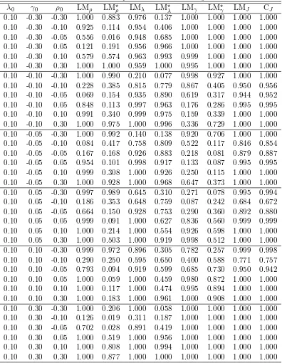
-0.30 0.046 0.015 0.042 0.005 0.047 0.016 0.042 0.008 -0.10 0.044 0.038 0.042 0.039 0.040 0.042 0.041 0.037 -0.05 0.040 0.049 0.048 0.051 0.043 0.045 0.047 0.046 0.05 0.061 0.046 0.061 0.056 0.057 0.051 0.056 0.052 0.10 0.074 0.042 0.064 0.039 0.070 0.041 0.061 0.043 0.30 0.135 0.028 0.100 0.024 0.128 0.035 0.099 0.028

Queen

-0.30 0.063 0.020 0.053 0.012 0.062 0.018 0.049 0.011 -0.10 0.044 0.047 0.046 0.043 0.039 0.038 0.044 0.038 -0.05 0.049 0.053 0.051 0.048 0.044 0.048 0.042 0.044 0.05 0.055 0.046 0.058 0.051 0.062 0.049 0.055 0.050 0.10 0.075 0.050 0.060 0.050 0.070 0.045 0.061 0.043 0.30 0.099 0.012 0.062 0.017 0.083 0.015 0.051 0.020

To save space, the size results based on the 2WE model will be presented through the P value discrepancy plots whereas the size results based on the DPD, SSPD and SDPDW models will be

226

summarized in tables. Note that in our design we allow for 6 different values for λ0, γ0 and ρ0,

which would yield 216 P value discrepancy plots for each. Hence, when the null model is one of

228

Nominal size S iz e d is c r e p an c y −0.01 −0.005 0 0.005 0.01

0 0.02 0.04 0.06 0.08 0.1 LMρ LM⋆ ρ LMλ LM⋆ λ LMγ LM⋆ γ LMJ CJ

(a) Rook weight matrix and normal errors

Nominal size S iz e d is c r e p an c y −0.01 −0.005 0 0.005 0.01

0 0.02 0.04 0.06 0.08 0.1

LMρ LM⋆ ρ LMλ LM⋆ λ LMγ LM⋆ γ LMJ CJ

(b) Rook weight matrix and non-normal errors

Nominal size S iz e d is c r e p an c y

−0.01

−0.005

0

0.005

0.01

0 0.02 0.04 0.06 0.08 0.1

LMρ LM⋆ ρ LMλ LM⋆ λ LMγ LM⋆ γ LMJ CJ

(c) Queen weight matrix and normal errors

Nominal size S iz e d is c r e p an c y

−0.01 −0.005 0 0.005 0.01 0.015

0 0.02 0.04 0.06 0.08 0.1

LMρ LM⋆ ρ LMλ LM⋆ λ LMγ LM⋆ γ LMJ CJ

(d) Queen weight matrix and non-normal errors

Figure 1: Size discrepancy plots when (n, T) = (100,10).

deviations at this level only. The general observations on the size properties of tests from Figure 1

230

and Tables 2 through 4 are listed as follows.

1. Fisgure 1 presents the size discrepancy plots when the null model is 2WE. The results show

232

that all tests have little size distortions and their size discrepancies generally lie inside the 95% confidence interval. The size discrepancies are relatively larger in the case of queen weight

234

matrix and non-normal errors.

2. Table 2 provide some evidences on the magnitude of size distortions as a function of the size

236

of local misspecification of the alternative model, the DPD model. One would expect to see robust versions of the one directional tests, LM⋆_ρ and LM⋆_λ, to perform better than LMρ and

238

be the case. For example, when the value of γ0 is 0.05 in absolute value in the true model,

240

the actual size of the robust tests are very close to the nominal size of 5%. However, as the misspecification deteriorates, this property of the robust tests vanish as expected.

242

3. Similar results hold for Table 3 as well, the robust versions of the one directional tests, LM⋆_ρ and LM⋆_γ, perform better than LMρ and LMγ, respectively, when λ0 deviates locally from

244

zero in the null model.

4. Tables 4 and 5 confirms our previous findings: LM⋆_ρperform better than LMρ, whenλ0 and

246

γ0 deviate locally from zero. For example, in Table 4, when true values ofλ0 and γ0 are 0.1,

the actual size of LM⋆_ρis 0.045 at the 5% level in the case of normal errors, whereas the actual

248

size of LMρis 0.985.

5. Recall that the robust tests use the residuals from the estimation of 2WE model and

imple-250

ments a correction on the test statistics for a local misspecification of the alternative model, i.e., ignoring the spatial component(s). The bias in these residuals depends on the strength

252

of spatial dependence as well as on the connectedness of the weights matrix. Therefore, we can expect poor performance for the robust tests as spatial parameters deviate from zero

254

substantially in the alternative model.

6. Finally, Tables 2, 4 and 5 indicate that as the temporal dependence strengthens, i.e., the

mis-256

specification inγ0 gets larger in absolute value, the performance of the robust one-directional

tests deteriorates significantly relative to their non-robust counterparts. This is not surprising

258

in the sense that the bias in the residuals from the estimation of 2WE model increase as the dependence over time strengthens.

260

Table 3: Empirical sizes when H0: The SSPD model and (n, T) = (100,10)

Normal Distribution Gamma Distribution

λ0 LMρ LM⋆ρ LMγ LMγ⋆ LMρ LM⋆ρ LMγ LM⋆γ

Rook

-0.30 1.000 0.791 1.000 0.999 1.000 0.793 1.000 1.000 -0.10 0.913 0.051 0.334 0.184 0.913 0.048 0.335 0.168 -0.05 0.394 0.053 0.087 0.071 0.379 0.052 0.085 0.065 0.05 0.326 0.048 0.077 0.068 0.336 0.051 0.073 0.064 0.10 0.853 0.051 0.204 0.136 0.863 0.053 0.215 0.143 0.30 1.000 0.730 0.998 0.997 1.000 0.708 0.999 0.998

Queen

-0.30 0.994 0.134 0.604 0.431 0.997 0.144 0.614 0.451 -0.10 0.393 0.058 0.070 0.068 0.374 0.055 0.072 0.064 -0.05 0.134 0.052 0.056 0.057 0.132 0.047 0.049 0.049 0.05 0.171 0.046 0.073 0.063 0.187 0.045 0.060 0.054 0.10 0.550 0.053 0.103 0.071 0.539 0.055 0.116 0.073 0.30 0.999 0.202 0.972 0.970 0.999 0.195 0.972 0.969

5.2 Results on Power Properties

To investigate power properties of all tests, we use the approach described in Davidson and

MacK-262

cor-Table 4: Empirical sizes when H0: The SDPDW model and (n, T) = (100,10): Rook

Normal Distribution Gamma Distribution

λ0 γ0 LMρ LM⋆ρ LMρ LM⋆ρ

-0.30 -0.30 0.580 0.299 0.578 0.310 -0.30 -0.10 0.999 0.833 1.000 0.831 -0.30 -0.05 1.000 0.831 1.000 0.830 -0.30 0.05 1.000 0.772 1.000 0.778 -0.30 0.10 1.000 0.885 1.000 0.892 -0.30 0.30 1.000 1.000 1.000 1.000 -0.10 -0.30 0.120 0.045 0.118 0.043 -0.10 -0.10 0.466 0.039 0.466 0.039 -0.10 -0.05 0.734 0.046 0.751 0.048 -0.10 0.05 0.971 0.048 0.974 0.042 -0.10 0.10 0.990 0.047 0.987 0.049 -0.10 0.30 1.000 0.739 0.999 0.739 -0.05 -0.30 0.073 0.025 0.067 0.024 -0.05 -0.10 0.128 0.044 0.137 0.045 -0.05 -0.05 0.242 0.050 0.255 0.047 -0.05 0.05 0.515 0.051 0.502 0.048 -0.05 0.10 0.612 0.049 0.610 0.046 -0.05 0.30 0.819 0.219 0.835 0.215 0.05 -0.30 0.068 0.018 0.062 0.015 0.05 -0.10 0.121 0.046 0.115 0.036 0.05 -0.05 0.207 0.049 0.208 0.053 0.05 0.05 0.474 0.051 0.469 0.053 0.05 0.10 0.557 0.042 0.585 0.045 0.05 0.30 0.598 0.022 0.597 0.017 0.10 -0.30 0.133 0.031 0.134 0.035 0.10 -0.10 0.360 0.042 0.347 0.051 0.10 -0.05 0.639 0.053 0.639 0.056 0.10 0.05 0.956 0.054 0.957 0.055 0.10 0.10 0.985 0.045 0.985 0.046 0.10 0.30 0.990 0.151 0.991 0.157 0.30 -0.30 0.763 0.296 0.764 0.302 0.30 -0.10 0.976 0.746 0.970 0.768 0.30 -0.05 1.000 0.757 1.000 0.754 0.30 0.05 1.000 0.643 1.000 0.652 0.30 0.10 1.000 0.637 1.000 0.627 0.30 0.30 1.000 1.000 1.000 1.000

responding null hypothesis. Therefore, two experiments need to be carried out. First, the data

264

generating process under the alternative hypothesis is used to generate the edf of p-values. We denote the resulting edf byFe(x). Second, the data generating process satisfies the null hypothesis,

266

and as before Fb(x) denotes the resulting edf of p-values. Then, a size-power curve is generated by plotting Fe(xi) against Fb(xi) for i= 1, . . . , m. As stated in Davidson and MacKinnon (1998), the

268

Table 5: Empirical sizes when H0: The SDPDW model and (n, T) = (100,10): Queen

Normal Distribution Gamma Distribution

λ0 γ0 LMρ LM⋆ρ LMρ LM⋆ρ

-0.30 -0.30 0.223 0.021 0.227 0.017 -0.30 -0.10 0.670 0.125 0.662 0.118 -0.30 -0.05 0.935 0.153 0.934 0.153 -0.30 0.05 1.000 0.105 1.000 0.106 -0.30 0.10 1.000 0.067 1.000 0.065 -0.30 0.30 1.000 0.418 1.000 0.432 -0.10 -0.30 0.046 0.021 0.041 0.021 -0.10 -0.10 0.126 0.042 0.120 0.043 -0.10 -0.05 0.230 0.049 0.234 0.048 -0.10 0.05 0.541 0.045 0.533 0.050 -0.10 0.10 0.638 0.048 0.636 0.043 -0.10 0.30 0.675 0.021 0.670 0.019 -0.05 -0.30 0.043 0.020 0.045 0.020 -0.05 -0.10 0.058 0.039 0.062 0.042 -0.05 -0.05 0.092 0.048 0.094 0.047 -0.05 0.05 0.179 0.050 0.175 0.051 -0.05 0.10 0.221 0.053 0.210 0.049 -0.05 0.30 0.209 0.009 0.208 0.010 0.05 -0.30 0.121 0.024 0.117 0.021 0.05 -0.10 0.065 0.042 0.061 0.041 0.05 -0.05 0.105 0.045 0.114 0.043 0.05 0.05 0.264 0.050 0.274 0.050 0.05 0.10 0.344 0.049 0.364 0.042 0.05 0.30 0.477 0.049 0.484 0.047 0.10 -0.30 0.230 0.032 0.220 0.035 0.10 -0.10 0.157 0.044 0.153 0.042 0.10 -0.05 0.328 0.047 0.326 0.043 0.10 0.05 0.713 0.056 0.732 0.050 0.10 0.10 0.821 0.048 0.821 0.049 0.10 0.30 0.912 0.178 0.918 0.187 0.30 -0.30 0.866 0.028 0.858 0.030 0.30 -0.10 0.783 0.170 0.789 0.170 0.30 -0.05 0.977 0.194 0.974 0.204 0.30 0.05 1.000 0.231 1.000 0.241 0.30 0.10 1.000 0.350 1.000 0.351 0.30 0.30 1.000 1.000 1.000 1.000

For all our proposed tests, the power curves can be generated in several ways. For example,

270

the power curves can be generated when the null model is the 2WE model, and the alternative can be one of the DPD, SSPD, SDPDW and SDPD model. We will refer to this as Case 1. However,

272

this approach would yield several plots, for instance, 216 plots for the 2WE–SDPD combination. To save space, we instead summarize the results in Tables 6 through 8, where the level for all tests

274

considered as null models for one-directional tests and their robust counterparts. Therefore, we can

276

generate size power curves for these one directional tests, where the null model is one of the DPD, SSPD and SDPDW models and the alternative model is one of the SDPDW and SDPD models.

278

We will refer to this as Case 2. For example, we could investigate the size power curves for LMλ

and LM⋆_λ where the null model is the DPD model and the alternative model is SDPDW model.

280

Similarly, for LMλ and LM⋆λ, the null of the DPD and the alternative of the SDPD would yield

another size power curve. We chose to present some representative cases in Figures 2 and 3.10

282

The general observations from Tables 6 through 8 on the power properties of our proposed tests for Case 1 are listed as follows. To save space, we only present the normally distributed error case,

284

as the results for the gamma distributed error case are similar. Also, for the case of the SDPD model, we focus on some representative tables.

286

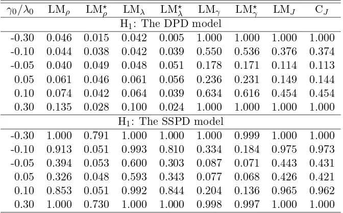
Table 6: Power of tests when H1: The DPD/SSPD model andH0: The 2WE model

γ0/λ0 LMρ LM⋆ρ LMλ LM⋆λ LMγ LM⋆γ LMJ CJ

H1: The DPD model

-0.30 0.046 0.015 0.042 0.005 1.000 1.000 1.000 1.000 -0.10 0.044 0.038 0.042 0.039 0.550 0.536 0.376 0.374 -0.05 0.040 0.049 0.048 0.051 0.178 0.171 0.114 0.113 0.05 0.061 0.046 0.061 0.056 0.236 0.231 0.149 0.144 0.10 0.074 0.042 0.064 0.039 0.634 0.616 0.454 0.454 0.30 0.135 0.028 0.100 0.024 1.000 1.000 1.000 1.000

H1: The SSPD model

-0.30 1.000 0.791 1.000 1.000 1.000 0.999 1.000 1.000 -0.10 0.913 0.051 0.993 0.810 0.334 0.184 0.975 0.973 -0.05 0.394 0.053 0.600 0.303 0.087 0.071 0.443 0.431 0.05 0.326 0.048 0.593 0.343 0.077 0.068 0.426 0.421 0.10 0.853 0.051 0.992 0.844 0.204 0.136 0.965 0.962 0.30 1.000 0.730 1.000 1.000 0.998 0.997 1.000 1.000

1. Table 6 shows that the joint test statistics and the one directional test statistics, LMγ, LM⋆γ

in the case of the DPD model and LMλ, LM⋆λ in the case of the SSPD model, have desirable

288

power.11

2. In Table 6, the robust versions of the one directional tests generally perform similar to their

290

non-robust counterparts. However, as the value ofγ0increases in the DPD model for example,

we see that the rejection frequencies of LM⋆_ρremain low whereas LMρover rejects the true null,

292

confirming the (over) size problem in Table 2. A similar finding applies to LM⋆_λ. Therefore, in case of temporal dependence in the data generating process, the robust tests are preferable.

294

In the case of the SSPD model in Table 6, LM⋆_γ and LM⋆_ρ report relatively smaller rejection frequencies and hence perform better than the non-robust counterparts. Again, in case of

296

spatial dependence in the data generating process, the robust tests are preferable.

10_{We only present results based on the rook weight matrix for the power analysis. The results based on the queen}

weight matrix are available upon request.

11_{Note that the one directional tests and their robust counterparts forλandρshould have lower rejection frequencies}

for the case where H1: The DPD model and H0: The 2WE model. Similarly, the one directional tests and their

robust counterparts forγ andρshould report lower rejection frequencies for the case where H1: The SSPD model

3. Table 7 reveals similar findings. The joint test statistics and the one directional test statistics,

298

LMγ, LM⋆γ and LMλ, LM⋆λ, have desirable power. LM⋆ρ’s rejection frequency remains low for

smaller deviations ofλ0 and γ0 from zero, whereas LMρover rejects the true null, confirming

300

the (over) size problem in Table 4. Therefore, in case of spatial and temporal dependence in the data generating process, the robust tests are preferable.

302

4. Tables 8, 9 and 10 shows that all one directional tests and the joint tests have proper power. The non-robust tests have higher power relative to their robust counterparts in some cases

304

but the differences are generally negligible.

For all our proposed tests, the power curves can be generated in several ways in Case 2. First,

306

one can obviously consider the 2WE model as the null model and the alternative can be one of the DPD, SSP, SDPDW and SDPD models. We will not generate size power curves for these cases as

308

we already summarized the results in Tables 6 through 10. Furthermore, for the one directional tests and their robust versions, one of the DPD, SSPD and SDPDW models can be the null model

310

and one of the SDPDW and SDPD models as the alternative model. For example, we can generate a size power curve for LMλ and LM⋆λ using the DPD model as the null model and the SDPDW

312

model as the alternative. Another size power curve for LMλ and LM⋆λ can be obtained from the

DPD model as the null model and the SDPD model as the alternative.12

314

In Figures 2 and 3, the lines with the red color correspond to the non-robust one directional test whereas the lines with blue color correspond to their robust counterparts. Different markers

316

are used to identify varying true values of the spatial parameter in the corresponding alternative model. The general observations on the power properties of our proposed tests are listed as follows.

318

12_{The experiments based on the gamma distributed errors are not presented, because results are similar to the}

Table 7: Power of tests when H1: The SDPDW model andH0: The 2WE model

λ0 γ0 LMρ LM⋆ρ LMλ LM⋆λ LMγ LM⋆γ LMJ CJ

Table 8: Power of tests when H1:The SDPD model andH0: The 2WE model

Normal distribution

λ0 γ0 ρ0 LMρ LM⋆ρ LMλ LM⋆λ LMγ LM⋆γ LMJ CJ

Table 9: Power of tests when H1: The SDPD model andH0: The 2WE model

λ0 γ0 ρ0 LMρ LM⋆ρ LMλ LM⋆λ LMγ LM⋆γ LMJ CJ

Table 10: Power of tests when H1: The SDPD model andH0: The 2WE model

Normal distribution

λ0 γ0 ρ0 LMρ LM⋆ρ LMλ LM⋆λ LMγ LM⋆γ LMJ CJ

Size

P

o

w

e

r

LMλ, LM⋆

λ:γ0= 0.1

0 0.2 0.4 0.6 0.8 1

0 0.2 0.4 0.6 0.8 1

λ0=−0.3

λ0=−0.1

λ0= 0.1

λ0= 0.3

(a) H0: The DPD model, H1: The SDPDW model

Size

P

o

w

e

r

LMλ, LM⋆λ:γ0= 0.1,ρ0=−0.1

0 0.2 0.4 0.6 0.8 1

0 0.2 0.4 0.6 0.8 1

λ0=−0.3

λ0=−0.1 λ0= 0.1

λ0= 0.3

(b) H0: The DPD model, H1: The SDPD model

Size

P

o

w

e

r

LMρ, LM⋆ρ:γ0= 0.1,λ0= 0.1

0

0.2

0.4

0.6

0.8

1

0 0.2 0.4 0.6 0.8 1

ρ0=−0.3 ρ0=−0.1 ρ0= 0.1 ρ0= 0.3

(c) H0: The DPD model, H1: The SDPD model

Size

P

o

w

e

r

LMγ, LM⋆γ:λ0= 0.1

0

0.2

0.4

0.6

0.8

1

0 0.2 0.4 0.6 0.8 1

γ0=−0.3

γ0=−0.1

γ0= 0.1

γ0= 0.3

(d) H0: The SSPD model, H1: The SDPDW model

Size

P

o

w

e

r

LMγ, LM⋆

γ:λ0= 0.1,ρ0=−0.1

0 0.2 0.4 0.6 0.8 1

0 0.2 0.4 0.6 0.8 1

γ0=−0.3 γ0=−0.1 γ0= 0.1

γ0= 0.3

(a) H0: The SSPD model, H1: The SDPD model

Size

P

o

w

e

r

LMρ, LM⋆ρ:λ0= 0.1,γ0= 0.1

0 0.2 0.4 0.6 0.8 1

0 0.2 0.4 0.6 0.8 1 ρ0=−0.3

ρ0=−0.1 ρ0= 0.1 ρ0= 0.3

(b) H0: The SSPD model, H1: The SDPD model

Size

P

o

w

e

r

LMρ, LM⋆_ρ:λ

0= 0.1,γ0= 0.1

0 0.2 0.4 0.6 0.8 1

0 0.2 0.4 0.6 0.8 1

ρ0=−0.3

ρ0=−0.1 ρ0= 0.1 ρ0= 0.3

(c) H0: The SDPDW model, H1: The SDPD model

Size

P

o

w

e

r

LMρ, LM⋆_{ρ:λ0= 0.3,γ0= 0.1}

0 0.2 0.4 0.6 0.8 1

0 0.2 0.4 0.6 0.8 1

ρ0=−0.3 ρ0=−0.1 ρ0= 0.1 ρ0= 0.3

(d) H0: The SDPDW model, H1: The SDPD model

1. In Figure 2(a), the null model is the DPD model and the alternative model is the SDPDW model. Both LMλ and LM⋆λ has satisfactory power. For lower values of λ0, LM⋆λ is less

320

powerful than LMλ. In Figure 2(b), the null model is the DPD model and the alternative

model is the SDPD model. Generally, LM⋆_λ is less powerful than LMλ except for the case

322

whereλ0= 0.1.

2. In Figure 2(c), the null model is the DPD model and the alternative model is again the

324

SDPD model. LM⋆_ρ is slightly less powerful than LMρ except for the case where ρ0 =−0.1.

In Figure 2(d), the null model is the SSPD model and the alternative model is again the

326

SDPDW model. LM⋆_γ and LMγ behave similarly and both lack power when γ0 =−0.1.

3. In Figure 3(a), the null model is the SSPD model and the alternative model is again the

328

SDPD model. Generally, LM⋆_γ and LMγ behave similarly. We see that when γ0 = 0.1, LM⋆γ

is more powerful than LMγ. But this picture reverses whenγ0=−0.1.

330

4. In Figure 3(b), the null model is the SSPD model and the alternative model is again the SDPD model. It confirms the results on the one directional tests of ρ0 from Table 3. LMρ

332

over rejects when the true model involves dependence over space and time. Furthermore, when spatial time lag coefficient is small on the negative side, LMρ suffers from positive size

334

distortion and lack of power. Surprisingly though, LM⋆_ρ lack power whenρ0 = 0.3.

5. In Figures 3(c) and 3(d), the null model is the SDPDW model and the alternative model is the

336

SDPD model. It confirms the results on the one directional tests ofρ0 from Table 4. Clearly,

LMρ over rejects when the true model involves dependence over space and time. Again, we

338

see that LM⋆_ρ lack power when ρ0 = 0.3. But, it does not suffer from size distortions unless

the misspecification in the alternative becomes larger.

340

6

Conclusion

In this paper, we introduce the robust LM tests within the GMM framework for a spatial dynamic

342

panel data model. These tests are robust in the sense that their asymptotic distributions under the null hypothesis are still a central chi-square distribution when the alternative model is misspecified.

344

On the other hand, when the alternative model is misspecified, the asymptotic null distributions of the standard LM tests deviate from the central chi-square distributions. Hence, the robust tests

346

obtain asymptotically the correct size. We derive the asymptotic distributions of our proposed tests under the null and the local alternative hypotheses. These tests can be used to test the presence of

348

the contemporaneous dependence over space, dependence over time and spatial time dependence. Since these tests are robust to the misspecification of the alternative models, they are much more

350

suitable for the detection of the source of dependence in a spatial dynamic panel data model. One attractive feature of our proposed tests is that their test statistics are easy to compute and

352

only require the estimates from a two-way error model. Therefore, our proposed tests can easily be made available for the practical applications by using the standard statistical softwares. In a

354

Monte Carlo study, we investigate the size and power properties of our proposed tests. Our results shows that the robust tests have good finite sample properties and would be useful for the detection

356

of the source of dependence in a spatial dynamic panel data model. The simulation results, hence, confirm our analytical results that the robust tests are valid, when the alternative models locally

358

Appendix

360

A

A Useful Lemma

Lemma 1. — Under our stated assumptions, the following results hold.

362

1. _N1EgnT(θ0)g

′

nT(θ0)

= ΣnT +o(1) and ΣbnT = ΣnT +op(1), where ΣbnT and ΣnT are stated

in the main text.

364

2. G(bθnT) =DnT+RnT+O

1

√

nT

, whereDnT isO(1), RnT isO(_T1) andbθnT is any consistent

estimator ofθ0.

366

3. G(bθnT)ΣbnTG(bθnT) = (DnT +RnT)

′

ΣnT (DnT +RnT) +op(1), where bθnT is any consistent

estimator ofθ0.

368

4. LetanT be a ka×(m+q) non-stochastic matrix. Then

1

√

NanTgnT(θ0)

d

−

→N0,plim_n→∞anTΣnTa

′

nT

(A.1)

Proof. See Lee and Yu (2014).

B

Expressions for Test Statistics

370

In this section, we provide explicit expressions for the elements of test statistics. Let thejth column ofGa(θ) be denoted byGa(θ) [:, j]. We start withG(θ) = (Gλ(θ), Gγ(θ), Gρ(θ), Gβ(θ)), where

Gλ(θ) [:, j] =−

1 N        

Y∗_n,T′ ₋₁W_nj,T′ ₋₁Jn,T−1P_ns_1,T−1Jn,T−1V∗_n,T−1(θ)

Y∗_n,T′ ₋₁W_nj,T′ ₋₁Jn,T−1Pns2,T−1Jn,T−1V∗n,T−1(θ)

.. .

Y_n,T∗′ ₋₁W′_nj,T−1Jn,T−1Psnm,T−1Jn,T−1Vn,T∗ −1(θ)

Q′_n,T−1Jn,T−1Wnj,T−1Yn,T∗ −1

        . (B.1)

Gγ(θ) =−

1 N         

V∗_n,T′ ₋₁(θ)Jn,T−1Ps_n1,T−1Jn,T−1Y_n,T(∗,−₋1)₁

V∗_n,T′ ₋₁(θ)Jn,T−1Ps_n2,T−1Jn,T−1Y_n,T(∗,−₋1)₁

.. .

V∗_n,T′ ₋₁(θ)Jn,T−1Pnm,Ts −1Jn,T−1Y(_n,T∗,−₋1)₁

Q′_n,T−1Jn,T−1Y_n,T(∗,−₋1)₁

         . (B.2)

Gρ(θ) [:, j] =−

1 N         

V∗_n,T′ ₋₁(θ)Jn,T−1Psn1,T−1Jn,T−1Wnj,T−1Y(_n,T∗,−₋1)₁

V∗_n,T′ ₋₁(θ)Jn,T−1Ps_n2,T−1Jn,T−1Wnj,T−1Y(_n,T∗,−₋1)₁

.. .

V_n,T∗′ ₋₁(θ)Jn,T−1Psnm,T−1Jn,T−1Wnj,T−1Y_n,T(∗,−₋1)₁

Q′_n,T−1Jn,T−1Wnj,T−1Y(_n,T∗,−₋1)₁

Gβ(θ) =− 1 N        

V∗_n,T′ ₋₁(θ)Jn,T−1Psn1,T−1Jn,T−1X∗n,T−1

V∗_n,T′ ₋₁(θ)Jn,T−1Ps_n2,T−1Jn,T−1X∗_n,T−1

.. .

V∗_n,T′ ₋₁(θ)Jn,T−1Ps_nm,T−1Jn,T−1X∗_n,T−1

Q′_n,T−1Jn,T−1X∗n,T−1

        . (B.4)

Using the inverse of the partitioned matrix formula (Amemiya 1985, p.460), we have

b Σ−_nT1 =

1

N

h b

σ4∆nm,T + bµ4−3σb4

ω′_nm,Tωnm,T

i

0m×q

0q×m σb2 1_NQ

′

n,T−1Jn,T−1Qn,T−1

!−1

=

O11 O12

O21 O22

, (B.5)

where O11 = Nσb4∆nm,T + µb4−3bσ4

ω_nm,T′ ωnm,T−1, O12 = O

′

21 = 0m×q, and O22 =

N

b

σ2

Q′_n,T−1Jn,T−1Qn,T−1−1. The component of C(θ) are given by

1. Cλ(θ) =G

′

λ(θ)

O11 O12

O21 O22

g_nT(θ), Cγ(θ) =G

′

γ(θ)

O11 O12

O21 O22

g_nT (θ) (B.6)

2. Cρ(θ) =G

′

ρ(θ)

O11 O12

O21 O22

g_nT(θ), Cβ(θ) =G

′

β(θ)

O11 O12

O21 O22

g_nT(θ) (B.7)

The components of B(θ) are defined in below.

1. Bλ(θ) =G

′

λ(θ)

O11 O12

O21 O22

Gλ, Bλρ(θ) =B

′

ρλ(θ) =G

′

λ(θ)

O11 O12

O21 O22

Gρ

2. Bλγ(θ) =B

′

γλ(θ) =G

′

λ(θ)

O11 O12

O21 O22

Gγ, Bλβ(θ) =B

′

βλ(θ) =G

′

λ(θ)

O11 O12

O21 O22

Gβ

3. Bρ(θ) =G

′

ρ(θ)

O11 O12

O21 O22

Gρ, Bργ(θ) =B

′

γρ(θ) =G

′

ρ(θ)

O11 O12

O21 O22

Gγ

4. Bρβ(θ) =B

′

βρ(θ) =G

′

ρ(θ)

O11 O12

O21 O22

Gβ, Bγ(θ) =G

′

γ(θ)

O11 O12

O21 O22

Gγ

5. Bγβ(θ) =B

′

βγ(θ) =G

′

γ(θ)

O11 O12

O21 O22

Gβ, Bβ(θ) =G

′

γ(θ)

O11 O12

O21 O22

Gβ.

Expressions for Hλ

0 :λ0 = 0:

C_λ⋆ θ˜nT=Cλ θ˜nT−Bλφ·β θ˜nTB_φ−_·1_β θ˜nTCφ θ˜nT, (B.8)

whereφ= ρ′, γ′,Cφ θ˜nT= C

′

ρ θ˜nT, C

′

γ θ˜nT

′

, and