Precision measurement of the Bºs Bºs oscillation frequency with the decay Bºs → Dsπ+

Original citation:

LHCb Collaboration (Including: Back, John J., Craik, Daniel, Dossett, D., Gershon, Timothy J., Harrison, Paul F., Kreps, Michal, Latham, Thomas, Pilar, T., Poluektov, Anton, Reid, Matthew M., Silva Coutinho, R., Whitehead, M. (Mark) and Williams, M. P.). (2013) Precision measurement of the Bs-0 Bs 0 oscillation frequency with the decay Bs- 0→ Dsπ -+. New Journal of Physics, Volume 15. Article number 053021

Permanent WRAP url:

http://wrap.warwick.ac.uk/57218

Copyright and reuse:

The Warwick Research Archive Portal (WRAP) makes this work of researchers of the University of Warwick available open access under the following conditions.

This article is made available under the Creative Commons Attribution- 3.0 Unported (CC BY 3.0) license and may be reused according to the conditions of the license. For more details seehttp://creativecommons.org/licenses/by/3.0/

A note on versions:

The version presented in WRAP is the published version, or, version of record, and may be cited as it appears here.

This content has been downloaded from IOPscience. Please scroll down to see the full text.

Download details:

IP Address: 137.205.202.184

This content was downloaded on 14/10/2013 at 14:14

Please note that terms and conditions apply.

Precision measurement of the B0s– oscillation frequency with the decay B0s → D−s+

View the table of contents for this issue, or go to the journal homepage for more 2013 New J. Phys. 15 053021

Precision measurement of the B

0_s

–B

0_s

oscillation

frequency with the decay B

0_s

→

D

−

_s

π

+

The LHCb Collaboration

New Journal of Physics15(2013) 053021 (15pp)

Received 18 April 2013 Published 14 May 2013 Online athttp://www.njp.org/

doi:10.1088/1367-2630/15/5/053021

E-mail:[email protected]

Abstract. A key ingredient to searches for physics beyond the Standard Model

in B0_smixing phenomena is the measurement of the B0_s– B0_s oscillation frequency, which is equivalent to the mass difference1msof the B0smass eigenstates. Using

the world’s largest B0

s meson sample accumulated in a dataset, corresponding

to an integrated luminosity of 1.0 fb−1, collected by the LHCb experiment at the CERN LHC in 2011, a measurement of1m_s is presented. A total of about 34 000 B0

s→D−sπ+signal decays are reconstructed, with an average decay time

resolution of 44 fs. The oscillation frequency is measured to be1m_s=17.768±

0.023 (stat)±0.006 (syst) ps−1_{, which is the most precise measurement to date.}

New Journal of Physics15(2013) 053021

1367-2630/13/053021+15$33.00

Contents

1. Introduction 2

2. The LHCb experiment 3

3. Signal selection and analysis strategy 4

4. Invariant mass description 5

5. Decay time description 6

6. Flavour tagging 7

7. Measurement of1ms 8

8. Systematic uncertainties 9

9. Conclusion 10

Acknowledgments 10

The LHCb Collaboration 10

References 14

1. Introduction

The Standard Model (SM) of particle physics, despite its great success in describing experimental data, is considered an effective theory valid only at low energies, below the TeV scale. At higher energies, new physics phenomena are predicted to emerge. For analyses looking for physics beyond the SM (BSM), there are two conceptually different approaches: direct and indirect searches. Direct searches are performed at the highest available energies and aim at producing and detecting new heavy particles. Indirect searches focus on precision measurements of quantum-loop-induced processes. Accurate theoretical predictions are available for the heavy quark sector in the SM. It is therefore an excellent place to search for new phenomena [1, 2], since any deviation from these predictions can be attributed to contributions from BSM.

In the SM, transitions between quark families (flavours) are possible via the charged current weak interaction. Flavour changing neutral currents (FCNC) are forbidden at lowest order, but are allowed in higher order processes. Since new particles can contribute to these loop diagrams, such processes are highly sensitive to contributions from BSM. An example FCNC transition is neutral meson mixing, where neutral mesons can transform into their antiparticles. Particle–antiparticle oscillations have been observed in the K0_–K0_{system [3], the B}0_–B0_system

[4], the B0_s–B0_s system [5,6] and the D0–D0system [7–10]. The frequency of B0_s– B0_s oscillations is the highest. On average, a B0_s meson changes its flavour nine times between production and decay. This poses a challenge to the detector for the measurement of the decay time. Another key ingredient of this measurement is the determination of the flavour of the B0

s meson at production,

which relies heavily on good particle identification and the separation of tracks from the primary interaction point.

The observed particle and antiparticle states B0_s and B0_s are linear combinations of the mass eigenstates BHand BL with massesmHandmLand decay widths0Hand0L, respectively [11].

asymmetries involving B0

s mesons, such as the B0s mixing phase φs in the decay B0s →

J/ψφ [12]. It was first observed by the Collider Detector at Fermilab (CDF) [6]. The Large Hadron Collider beauty experiment (LHCb) published a measurement of this frequency using a dataset, corresponding to an integrated luminosity of 37 pb−1, taken in 2010 [13]. This analysis complements the previous result and is obtained in a similar way, using a data sample, corresponding to an integrated luminosity of 1.0 fb−1, collected by LHCb in 2011.

2. The LHCb experiment

The LHCb experiment is designed for precision measurements in the beauty and charm hadron systems. At a centre-of-mass energy of√s₌7 TeV, about 3×1011_{bb pairs were produced in}

2011. The LHCb detector [14] is a single-arm forward spectrometer covering the pseudorapidity range from two to five. The excellent decay time resolution necessary to resolve the fast B0_s– B0_s oscillation is provided by a silicon-strip vertex detector surrounding the pp interaction region. At nominal position, the sensitive region of the vertex detector is only 8 mm away from the beam. An impact parameter (IP) resolution of 20µm for tracks with high transverse momentum (pT) is achieved.

Charged particle momenta are measured with the LHCb tracking system consisting of the aforementioned vertex detector, a large-area silicon-strip detector located upstream of a dipole magnet with a bending power of about 4 T m, and three stations of silicon-strip detectors and straw drift tubes placed downstream. The combined tracking system has momentum resolution 1p/pthat varies from 0.4% at 5 GeV/cto 0.6% at 100 GeV/c.

Since this analysis is performed with decays involving only hadrons in the final state, excellent particle identification is crucial to suppress background. Charged hadrons are identified using two ring-imaging Cherenkov detectors [15]. Photon, electron and hadron candidates are identified by a calorimeter system consisting of scintillating-pad and preshower detectors, an electromagnetic calorimeter and a hadronic calorimeter. Muons are identified by a system composed of alternating layers of iron and multiwire proportional chambers.

The first stage of the trigger [16] is implemented in hardware, based on information from the calorimeter and muon systems, and selects events that contain candidates with large transverse energy and transverse momentum. This is followed by a software stage that applies a full event reconstruction. The software trigger used in this analysis requires a two-, three-or four-track secondary vertex with a significant displacement from the primary interaction, a large sum of p_T of the tracks, and at least one track with p_T>1.7 GeV/c. In addition, an IPχ2

with respect to the primary interaction greater than 16 and a track fitχ2_{per degree of freedom}

<2 is required. The IP χ2 _{is defined as the difference between the} χ2 _{of the primary vertex}

reconstructed with and without the considered track. A multivariate algorithm is used for the identification of the secondary vertices.

3. Signal selection and analysis strategy

The analysis uses B0_s candidates reconstructed in the flavour-specific decay mode1B0_s →D−_sπ+ in five D−

s decay modes, namely D−s →φ(K+K−)π−, D−s →K∗0(K+π−)K−, D−s →K+K−π−

nonresonant, D−

s →K−π+π− and D−s →π−π+π−. To avoid double counting, events that

contain a candidate passing the selection criteria of one mode are not considered for the subsequent modes, using the order listed above. All reconstructed decays are flavour-specific final states; thus the flavour of the B0

s candidate at the time of its decay is given by the charges of

the final state particles. A combination of tagging algorithms is used to identify the B0

s flavour at

production. The algorithms provide for each candidate a tagging decision as well as an estimate of the probability that this decision is wrong (mistag probability). These algorithms have been optimized using large event samples of flavour-specific decays [24,25].

To be able to study the effect of selection criteria that influence the decay time spectrum, we restrict the analysis to those events in which the signal candidate passed the requirements of the software trigger algorithm used in this analysis. Specific features, such as the masses of the intermediateφ and K∗0 resonances or the Dalitz structure of the D−_s →π−π+π− decay mode, are exploited for the five decay modes. The most powerful quantity to separate signal from background common to all decay modes is the output of a boosted decision tree (BDT) [26]. The BDT exploits the long B0

s lifetime by using as input the IP χ2 of the daughter tracks, the

angle of the reconstructed B0

s momentum relative to the line between the reconstructed primary

vertex, and the B0

s vertex and the radial flight distance in the transverse plane of both the B0s and

the D−

s mesons. Additional requirements are applied on the sum of the pTof the B0s candidate’s

decay products as well as on particle identification variables, and on track and vertex quality. The reconstructed D−

s mass is required to be consistent with the known value [27]. After this

selection, a total of about 47 800 candidates remain in the B0_s→D−_sπ+invariant mass window of 5.32–5.98 GeV/c2.

An unbinned likelihood method is employed to simultaneously fit the B0_s invariant mass and decay time distributions of the five decay modes. The probability density functions (PDFs) for signal and background in each of the five modes can be written as

P₌Pm(m)Pt(t,q|σt, η)Pσt(σt)Pη(η), (1)

where m is the reconstructed invariant mass of the B0

s candidate, t is its reconstructed decay

time andσt is an event-by-event estimate of the decay time resolution. The tagging decisionq can be 0 if no tag is found,−1 for events with different flavour at production and decay (mixed) or +1 for events with the same flavour at production and decay (unmixed). The predicted event-by-event mistag probability η can take values between 0 and 0.5. The functions Pm and Pt describe the invariant mass and the decay time probability distributions, respectively. Pt is a conditional probability depending onσt andη. The functionsPσt andPη are required to ensure

the proper relative normalization of Pt for signal and background [28]. The functionsPσt and

P_η are determined from data, using the measured distribution in the upper B0_s invariant mass sideband for the background PDF and the sideband subtracted distribution in the invariant mass signal region for the signal PDF.

This measurement has been performed ‘blinded’, meaning that during the analysis process the fitted value of1mswas shifted by an unknown value, which was removed after the analysis

procedure had been finalized.

]

2

c ) invariant mass [MeV/

+

π −

s

(D

5350 5400 5450 5500 5550

)

2

c

candidates / (15 MeV/

0 2000 4000 data fit + π − s D → 0 s B + K − s D → 0 s B misid bkg. comb bkg. a)

LHCb

− π φ → − s D ] 2 c ) invariant mass [MeV/

+

π −

s

(D

5350 5400 5450 5500 5550

)

2

c

candidates / (15 MeV/

0 2000 data fit + π − s D → 0 s B + K − s D → 0 s B misid. bkg. comb. bkg. − K*K → − s D

LHCb

b) ] 2 c ) invariant mass [MeV/

+

π −

s

(D

5350 5400 5450 5500 5550

)

2

c

candidates / (15 MeV/

0 1000 2000 data fit + π − s D → 0 s B + K − s D → 0 s B misid. bkg. comb. bkg. − π − K + K → − s D

LHCb

c) ] 2 c ) invariant mass [MeV/

+

π −

s

(D

5350 5400 5450 5500 5550

)

2

c

candidates / (15 MeV/

0 500 data fit + π − s D → 0 s B + K − s D → 0 s B misid. bkg. comb. bkg. − π + π − K → − s D

LHCb

d) ] 2 c ) invariant mass [MeV/

+

π −

s

(D

5350 5400 5450 5500 5550

)

2

c

candidates / (15 MeV/

[image:7.595.148.526.83.445.2]

0 1000 data fit + π − s D → 0 s B + K − s D → 0 s B comb. bkg. − π − π + π → − s D

LHCb

e)

Figure 1. Invariant mass distributions for B0

s →D−sπ+ candidates with the D−s

meson decaying as (a) D−

s →φ(K+K−)π−, (b) D−s →K∗0(K+π−)K−, (c) D−s →

K+_K−π− _{nonresonant, (d) D}−

s →K−π+π− and (e) D−s →π−π+π−. The fits

and the various background components are described in the text. Misidentified backgrounds refer to background from B0_and30

bdecays with one misidentified daughter particle.

4. Invariant mass description

The invariant mass of each B0

s candidate is determined in a vertex fit constraining the D−s

invariant mass to its known value [27]. The invariant mass spectra for the five decay modes after all the selection criteria are applied are shown in figure 1. The fit to the five distributions takes into account contributions from signal, combinatorial background and b-hadron decay backgrounds. The signal components are described by the sum of two Crystal Ball (CB) functions [29], which are constrained to have the same peak parameter. The parameters of the CB function describing the tails are fixed to values obtained from simulation, whereas the mean and the two widths are allowed to vary. These are constrained to be the same for all five decay modes. It has been checked on data that the mass resolution is compatible among all modes.

[image:8.595.151.491.148.252.2]

Table 1. Number of candidates and B0_s signal fractions in the mass range 5.32–5.98 GeV/c2.

Decay mode (D−

sπ+) candidates fB0

s→D−sπ+ fB0s→D∓sK±

D−_s →φ(K+K−)π− 14 691 0.834±0.008

D−

s →K∗0(K+π−)K− 10 866 0.857±0.009

D−

s →K+K−π−nonresonant 11 262 0.595±0.009

D−

s →K−π

+_{π− 4288 0.437}

±0.014

D−

s →π−π+π− 6674 0.599±0.008 0.019±0.010

Total 47 781 0.714±0.004 0.019±0.010

different b-hadron decay backgrounds are allowed to vary individually for each of the five decay modes. Another component originates from B0_s→D∓

sK± decays, in which the kaon is

misidentified as a pion. This contribution is treated as a signal in the decay time analysis. The requirement that the invariant mass be larger than 5.32 GeV/c2 rejects background candidates from B0_s decays with additional particles in the decay not reconstructed, such as B0_s →D∗−_s π+(D_s∗−→D−_sπ0 or D−_sγ). The fitted number of signal candidates does not change with respect to a fit in a larger mass window. The high mass sideband region 5.55–5.98 GeV/c2 provides a sample of mainly combinatorial background candidates. The mass distribution is described by an exponential function, whose parameters are allowed to vary individually for the five decay modes. By including this region in the fit, we are able to determine the decay time distribution as well as the tagging behaviour of the combinatorial background.

The number of used candidates along with the signal fractions extracted from the two-dimensional fit in mass and decay time are reported in table 1. One complication arises from the fact that the shape of the invariant mass distribution of the B0_s →D∓

sK± events is very

similar to that of the B0 background. Therefore, the fraction of B0_s→D∓

sK± candidates has

been determined in a fit to the D−_s →π−π+π−mode only, in which no B0background is present. Subsequently this value is used for all the other modes.

5. Decay time description

The decay time of a particle is measured as

t ₌ Lm

p , (2)

where L is the distance between the production vertex and the decay vertex of the particle, m its reconstructed invariant mass and pits reconstructed momentum. We use the decay time calculated without the D−

s mass constraint to avoid a systematic dependence of the B0s decay time

on the reconstructed invariant mass. The theoretical distribution of the decay time, t, ignoring the oscillation and any detector resolution, is

Pt ∝0se−0st cosh 10

s

2 t

where 0s is the B0s decay width and 10s the decay width difference between the light and

heavy mass eigenstates2_{. The value for}10

sis fixed to the latest value measured by LHCb [12]

10s=0.106±0.011±0.007 ps−1. It is varied within its uncertainties to assess the systematic

effect on the measurement of1m_s. The Heaviside step functionθ(t)restricts the PDF to positive decay times.

To account for detector resolution effects, the decay time PDF is convolved with a Gaussian distribution. The width σt is taken from an event-by-event estimate returned by the fitting algorithm that reconstructs the B0_s decay vertex. Due to tracking detector resolution effects,σt needs to be calibrated. A data-driven method, combining prompt D−

s mesons from the primary

interaction with random π+ _{mesons, forms fake B}0

s candidates. The decay time distribution of

these candidates, each divided by its event-by-eventσt, is fitted with a Gaussian function. The width provides a scale factor S_{σt =}1.37, by which eachσt is multiplied, such that it represents the correct resolution. By inspecting different regions of phase space of the fake B0

s candidates,

the uncertainty range on this number is found to be 1.25<S_σt <1.45. The variation is taken into account as part of the1m_ssystematic studies. The resulting average decay time resolution is S_{σt × h}σti =44 fs.

Some of the selection criteria influence the shape of the decay time distribution, e.g. the requirement of a large IP for B0_s daughter tracks. Thus, a decay time acceptance functionEt(t) has to be taken into account. Its parametrization is determined from simulated data and the parameter describing its shape is allowed to vary in the fit to the data, while 0s is fixed to the

nominal value [27]. Taking into account resolution and decay time acceptance, the PDF given in equation (3) is modified to

Pt(t|σt)∝

0se−0st cosh 10

s

2 t

θ(t)

⊗G(t_;0,S_σtσt)Et(t) (4)

with G(t_;0,S_σtσt) being the resolution function determined by the method mentioned above. The decay time PDFs for the B0and30b backgrounds are identical to the signal PDF, except for 10 being zero, and0sbeing replaced by their respective decay widths [27]. The shape of the

decay time distribution of the combinatorial background is determined with high mass sideband data. It is parametrized by the sum of two exponential functions multiplied by a second-order polynomial distribution. The exponential and polynomial parameters are allowed to vary in the fit and are constrained to be the same for the five decay modes.

6. Flavour tagging

To determine the flavour of the B0_s meson at production, both opposite-side (OST) and same-side (SST) tagging algorithms are used. The OST exploits the fact that b quarks at the LHC are predominantly produced in quark–antiquark pairs. By partially reconstructing the second b hadron in the event, conclusions on the flavour at production of the signal B0_s candidate can be drawn. The OST has been optimized on large samples of B+

→J/ψK+, B_→µ+_D∗−_{X and}

B0

→D−_π+_{decays [24].}

The SST takes advantage of the fact that the net strangeness of the pp collision is zero. Therefore, thesquark needed for the hadronization of the B0

smeson must have been produced in

association with ansquark, which in about 50% of the cases hadronizes to form a charged kaon.

2 _10sand1m

By identifying this kaon, the flavour at production of the signal B0

s candidate is determined. The

optimization of the SST was performed on a data sample of B0

s →D−sπ+ decays, which has a

large overlap with the sample used in this analysis [25]. However, since the oscillation frequency is not correlated with the parameters describing tagging performance, this does not bias the1m_s measurement.

The decisions given by both tagging algorithms have a probabilityωto be incorrect. Each tagging algorithm provides an estimate for the mistag probability η; which is the output of a neural network combining various event properties. The true mistag probability ω can be parametrized as a linear function of the estimateη[24,25]:

ω= p₀+p_1×(η_{− h}η_i) (5)

withhηibeing the mean of the distribution ofη. This parametrization is chosen to minimize the correlations between p0and p1. The calibration is performed separately for the OST and SST.

The sets of calibration parameters(p0,p1)OSTand(p0,p1)SSTare allowed to vary in the fit.

The figure of merit of these tagging algorithms is called the effective tagging efficiencyεeff. It

gives the factor by which the statistical power of the sample is reduced due to imperfect tagging decisions. In this analysis,εeffis found to be(2.6±0.4)% for the OST and(1.2±0.3)% for the

SST. Uncertainties are statistical only.

7. Measurement of1ms

Adding the information of the flavour tagging algorithms, the decay time PDF for tagged signal candidates is modified to

Pt(t|σt)∝

0se−0st

1 2

cosh

10 s

2 t

+q[1−2ω(ηOST, ηSST)] cos(1mst)

θ(t)

⊗G(t,S_σtσt)Et(t) , (6) where gives the fraction of candidates with a tagging decision. Signal candidates without a tagging decision are still described by equation (4) multiplied by an additional factor(1−)to ensure relative normalization.

The information provided by the opposite-side and same-side taggers for the signal is combined to a single tagging decisionqand a single mistag probabilityω(ηOST,ηSST)using their

respective calibration parameters p0OST/SST and p1OST/SST. The individual background components show different tagging characteristics for candidates tagged by the OST or SST. The bhadron backgrounds show the same opposite-side tagging behaviour (q and ω) as the signal, while the combinatorial background shows random tagging behaviour. For same-side tagged events, we assume random tagging behaviour for all background components. We introduce tagging asymmetry parameters to allow for different numbers of candidates being tagged as mixed or unmixed, and other parameters to describe the tagging efficiencies for these backgrounds. As expected, the fitted values of these asymmetry parameters are consistent with zero within uncertainties.

decay time [ps]

0 1 2 3 4

candidates / (0.1 ps)

0 200 400

Tagged mixed

Tagged unmixed

Fit mixed

Fit unmixed

[image:11.595.148.412.101.265.2]

LHCb

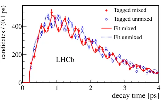
Figure 2. Decay time distribution for the sum of the five decay modes for candidates tagged as mixed (different flavour at decay and production; red, continuous line) or unmixed (same flavour at decay and production; blue, dotted line). The data and the fit projections are plotted in a signal window around the reconstructed B0_s mass of 5.32–5.55 GeV/c2.

8. Systematic uncertainties

With respect to the first measurement of 1m_s at LHCb [13], all sources of systematic uncertainties have been reevaluated.

The dominant source is related to the knowledge of the absolute value of the decay time. This has two main contributions. First, the imperfect knowledge of the longitudinal (z) scale of the detector contributes to the systematic uncertainty. It is obtained by comparing the track-based alignment and survey data and evaluating the track distribution in the vertex detector. This results in 0.02% uncertainty on the decay time scale and thus an absolute uncertainty of

±0.004 ps−1 _on1m s.

The second contribution to the uncertainty of the decay time scale comes from the knowledge of the overall momentum scale. This has been evaluated by an independent study using mass measurements of well-known resonances. Deviations from the reference values [27] are measured to be within 0.15%. However, since both the measured invariant mass and momentum enter the calculation of the decay time, this effect cancels to some extent. The resulting systematic uncertainty on the decay time scale is evaluated from simulation to be 0.02%. This again translates to an absolute uncertainty of±0.004 ps−1_on1m

s.

The next largest systematic uncertainty is due to a possible bias of the measured decay time given by the track reconstruction and the selection procedure. This is estimated from simulated data to be less than about 0.2 fs, and results in±0.001 ps−1systematic uncertainty on1ms.

Various other sources contributing to the systematic uncertainty have been studied such as the decay time acceptance, decay time resolution, variations of the value of 10s, different

signal models for the invariant mass and the decay time resolution, variations of the signal fraction and the fraction of B0

s→D∓sK± candidates. They are all found to be negligible. The

[image:12.595.147.350.148.224.2]

Table 2.Systematic uncertainties on the1m_smeasurement. The total systematic uncertainty is calculated as the quadratic sum of the individual contributions.

Source Uncertainty (ps−1)

z-scale 0.004

Momentum scale 0.004

Decay time bias 0.001

Total systematic uncertainty 0.006

9. Conclusion

A measurement of the B0_s– B0_s oscillation frequency 1m_s is performed using B0_s →D−_sπ+ decays in five different D−_s decay channels. Using a data sample corresponding to an integrated luminosity of 1.0 fb−1collected by LHCb in 2011, the oscillation frequency is found to be

1ms=17.768±0.023(stat)±0.006(syst)ps−1,

in good agreement with the first result reported by the LHCb experiment [13] and the current world average, 17.69±0.08 ps−1 _{[27]. This is the most precise measurement of} 1_m

s to date,

and will be a crucial ingredient in future searches for BSM physics in B0

s oscillations.

Acknowledgments

We express our gratitude to our colleagues in the CERN accelerator departments for the excellent performance of the LHC. We thank the technical and administrative staff at the LHCb institutes. We acknowledge support from CERN and from the national agencies: CAPES, CNPq, FAPERJ and FINEP (Brazil); NSFC (China); CNRS/IN2P3 and Region Auvergne (France); BMBF, DFG, HGF and MPG (Germany); SFI (Ireland); INFN (Italy); FOM and NWO (The Netherlands); SCSR (Poland); ANCS/IFA (Romania); MinES, Rosatom, RFBR and NRC ‘Kurchatov Institute’ (Russia); MinECo, XuntaGal and GENCAT (Spain); SNSF and SER (Switzerland); NAS Ukraine (Ukraine); STFC (UK); and NSF (USA). We also acknowledge the support received from the ERC under FP7. The Tier1 computing centres are supported by IN2P3 (France), KIT and BMBF (Germany), INFN (Italy), NWO and SURF (The Netherlands), PIC (Spain) and GridPP (UK). We are thankful for the computing resources put at our disposal by Yandex LLC (Russia), as well as to the communities behind the multiple open source software packages that we depend on.

The LHCb Collaboration

R Aaij40_{, C Abellan Beteta}35,73_{, B Adeva}36_{, M Adinolfi}45_{, C Adrover}6_{, A Affolder}51_,

A Berezhnoy31_{, R Bernet}39_{, M-O Bettler}46_{, M van Beuzekom}40_{, A Bien}11_{, S Bifani}44_{, T Bird}53_,

A Bizzeti17,67_{, P M Bjørnstad}53_{, T Blake}37_{, F Blanc}38_{, J Blouw}11_{, S Blusk}57_{, V Bocci}24_,

A Bondar33, N Bondar29, W Bonivento15, S Borghi53, A Borgia57, T J V Bowcock51, E Bowen39, C Bozzi16, T Brambach9, J van den Brand41, J Bressieux38, D Brett53, M Britsch10, T Britton57, N H Brook45, H Brown51, I Burducea28, A Bursche39, G Busetto21,76, J Buytaert37, S Cadeddu15, O Callot7, M Calvi20,69, M Calvo Gomez35,73, A Camboni35, P Campana18,37, D Campora Perez37, A Carbone14,62, G Carboni23,70, R Cardinale19,68, A Cardini15, H Carranza-Mejia49, L Carson52, K Carvalho Akiba2, G Casse51, M Cattaneo37, Ch Cauet9_{, M Charles}54_{, Ph Charpentier}37_{, P Chen}3,38_{, N Chiapolini}39_{, M Chrzaszcz}25_,

K Ciba37_{, X Cid Vidal}37_{, G Ciezarek}52_{, P E L Clarke}49_{, M Clemencic}37_{, H V Cliff}46_,

J Closier37_{, C Coca}28_{, V Coco}40_{, J Cogan}6_{, E Cogneras}5_{, P Collins}37_{, A Comerma-Montells}35_,

A Contu15,37_{, A Cook}45_{, M Coombes}45_{, S Coquereau}8_{, G Corti}37_{, B Couturier}37_{, G A Cowan}49_,

D C Craik47_{, S Cunliffe}52_{, R Currie}49_{, C D’Ambrosio}37_{, P David}8_{, P N Y David}40_,

I De Bonis4_{, K De Bruyn}40_{, S De Capua}53_{, M De Cian}39_{, J M De Miranda}1_{, L De Paula}2_,

W De Silva56_{, P De Simone}18_{, D Decamp}4_{, M Deckenhoff}9_{, L Del Buono}8_{, D Derkach}14_,

O Deschamps5, F Dettori41, A Di Canto11, H Dijkstra37, M Dogaru28, S Donleavy51, F Dordei11, A Dosil Su´arez36, D Dossett47, A Dovbnya42, F Dupertuis38, R Dzhelyadin34, A Dziurda25, A Dzyuba29, S Easo48,37, U Egede52, V Egorychev30, S Eidelman33, D van Eijk40, S Eisenhardt49, U Eitschberger9, R Ekelhof9, L Eklund50,37, I El Rifai5, Ch Elsasser39, D Elsby44, A Falabella14,64, C F¨arber11, G Fardell49, C Farinelli40, S Farry12, V Fave38, D Ferguson49_{, V Fernandez Albor}36_{, F Ferreira Rodrigues}1_{, M Ferro-Luzzi}37_{, S Filippov}32_,

M Fiore16_{, C Fitzpatrick}37_{, M Fontana}10_{, F Fontanelli}19,68_{, R Forty}37_{, O Francisco}2_{, M Frank}37_,

C Frei37_{, M Frosini}17,65_{, S Furcas}20_{, E Furfaro}23,70_{, A Gallas Torreira}36_{, D Galli}14,62_,

M Gandelman2_{, P Gandini}57_{, Y Gao}3_{, J Garofoli}57_{, P Garosi}53_{, J Garra Tico}46_{, L Garrido}35_,

C Gaspar37_{, R Gauld}54_{, E Gersabeck}11_{, M Gersabeck}53_{, T Gershon}47,37_{, Ph Ghez}4_{, V Gibson}46_,

V V Gligorov37_{, C G¨obel}58_{, D Golubkov}30_{, A Golutvin}52,30,37_{, A Gomes}2_{, H Gordon}54_,

M Grabalosa G´andara5_{, R Graciani Diaz}35_{, L A Granado Cardoso}37_{, E Graug´es}35_{, G Graziani}17_,

A Grecu28, E Greening54, S Gregson46, O Gr¨unberg59, B Gui57, E Gushchin32, Yu Guz34,37, T Gys37, C Hadjivasiliou57, G Haefeli38, C Haen37, S C Haines46, S Hall52, T Hampson45, S Hansmann-Menzemer11, N Harnew54, S T Harnew45, J Harrison53, T Hartmann59, J He37, V Heijne40, K Hennessy51, P Henrard5, J A Hernando Morata36, E van Herwijnen37, E Hicks51, D Hill54, M Hoballah5, C Hombach53, P Hopchev4, W Hulsbergen40, P Hunt54, T Huse51, N Hussain54, D Hutchcroft51, D Hynds50, V Iakovenko43, M Idzik26, P Ilten12, R Jacobsson37, A Jaeger11_{, E Jans}40_{, P Jaton}38_{, F Jing}3_{, M John}54_{, D Johnson}54_{, C R Jones}46_{, B Jost}37_,

M Kaballo9_{, S Kandybei}42_{, M Karacson}37_{, T M Karbach}37_{, I R Kenyon}44_{, U Kerzel}37_{, T Ketel}41_,

A Keune38_{, B Khanji}20_{, O Kochebina}7_{, I Komarov}38_{, R F Koopman}41_{, P Koppenburg}40_,

M Korolev31_{, A Kozlinskiy}40_{, L Kravchuk}32_{, K Kreplin}11_{, M Kreps}47_{, G Krocker}11_,

P Krokovny33_{, F Kruse}9_{, M Kucharczyk}20,25,69_{, V Kudryavtsev}33_{, T Kvaratskheliya}30,37_,

V N La Thi38_{, D Lacarrere}37_{, G Lafferty}53_{, A Lai}15_{, D Lambert}49_{, R W Lambert}41_,

E Lanciotti37_{, G Lanfranchi}18_{, C Langenbruch}37_{, T Latham}47_{, C Lazzeroni}44_{, R Le Gac}6_,

A Massafferri1_{, R Matev}37_{, Z Mathe}37_{, C Matteuzzi}20_{, E Maurice}6_{, A Mazurov}16,32,37,64_,

J McCarthy44_{, A McNab}53_{, R McNulty}12_{, B Meadows}56,54_{, F Meier}9_{, M Meissner}11_,

M Merk40, D A Milanes8, M-N Minard4, J Molina Rodriguez58, S Monteil5, D Moran53, P Morawski25, M J Morello22,78, R Mountain57, I Mous40, F Muheim49, K M¨uller39, R Muresan28, B Muryn26, B Muster38, P Naik45, T Nakada38, R Nandakumar48, I Nasteva1, M Needham49, N Neufeld37, A D Nguyen38, T D Nguyen38, C Nguyen-Mau38,75, M Nicol7, V Niess5, R Niet9, N Nikitin31, T Nikodem11, A Nomerotski54, A Novoselov34, A Oblakowska-Mucha26, V Obraztsov34, S Oggero40, S Ogilvy50, O Okhrimenko43, R Oldeman15,63, M Orlandea28_{, J M Otalora Goicochea}2_{, P Owen}52_{, A Oyanguren} 35,74_{, B K Pal}57_,

A Palano13,61_{, M Palutan}18_{, J Panman}37_{, A Papanestis}48_{, M Pappagallo}50_{, C Parkes}53_,

C J Parkinson52_{, G Passaleva}17_{, G D Patel}51_{, M Patel}52_{, G N Patrick}48_{, C Patrignani}19,68_,

C Pavel-Nicorescu28_{, A Pazos Alvarez}36_{, A Pellegrino}40_{, G Penso}24,71_{, M Pepe Altarelli}37_,

S Perazzini14,62_{, D L Perego}20,69_{, E Perez Trigo}36_{, A P´erez-Calero Yzquierdo}35_{, P Perret}5_,

M Perrin-Terrin6_{, G Pessina}20_{, K Petridis}52_{, A Petrolini}19,68_{, A Phan}57_{, E Picatoste Olloqui}35_,

B Pietrzyk4_{, T Pilaˇr}47_{, D Pinci}24_{, S Playfer}49_{, M Plo Casasus}36_{, F Polci}8_{, G Polok}25_,

A Poluektov47,33, E Polycarpo2, D Popov10, B Popovici28, C Potterat35, A Powell54, J Prisciandaro38, V Pugatch43, A Puig Navarro38, G Punzi22,77, W Qian4, J H Rademacker45, B Rakotomiaramanana38, M S Rangel2, I Raniuk42, N Rauschmayr37, G Raven41, S Redford54, M M Reid47, A C dos Reis1, S Ricciardi48, A Richards52, K Rinnert51, V Rives Molina35, D A Roa Romero5, P Robbe7, E Rodrigues53, P Rodriguez Perez36, S Roiser37, V Romanovsky34, A Romero Vidal36_{, J Rouvinet}38_{, T Ruf}37_{, F Ruffini}22_{, H Ruiz}35_{, P Ruiz Valls}35,74_,

G Sabatino24,70_{, J J Saborido Silva}36_{, N Sagidova}29_{, P Sail}50_{, B Saitta}15,63_{, C Salzmann}39_,

B Sanmartin Sedes36_{, M Sannino}19,68_{, R Santacesaria}24_{, C Santamarina Rios}36_{, E Santovetti}23,70_,

M Sapunov6_{, A Sarti}18,71_{, C Satriano}24,72_{, A Satta}23_{, M Savrie}16,64_{, D Savrina}30,31_{, P Schaack}52_,

M Schiller41_{, H Schindler}37_{, M Schlupp}9_{, M Schmelling}10_{, B Schmidt}37_{, O Schneider}38_,

A Schopper37_{, M-H Schune}7_{, R Schwemmer}37_{, B Sciascia}18_{, A Sciubba}24_{, M Seco}36_,

A Semennikov30_{, K Senderowska}26_{, I Sepp}52_{, N Serra}39_{, J Serrano}6_{, P Seyfert}11_{, M Shapkin}34_,

I Shapoval16,42, P Shatalov30, Y Shcheglov29, T Shears51,37, L Shekhtman33, O Shevchenko42, V Shevchenko30, A Shires52, R Silva Coutinho47, T Skwarnicki57, N A Smith51, E Smith54,48, M Smith53, M D Sokoloff56, F J P Soler50, F Soomro18, D Souza45, B Souza De Paula2, B Spaan9, A Sparkes49, P Spradlin50, F Stagni37, S Stahl11, O Steinkamp39, S Stoica28, S Stone57, B Storaci39, M Straticiuc28, U Straumann39, V K Subbiah37, S Swientek9, V Syropoulos41, M Szczekowski27, P Szczypka38,37, T Szumlak26, S T’Jampens4, M Teklishyn7, E Teodorescu28, F Teubert37_{, C Thomas}54_{, E Thomas}37_{, J van Tilburg}11_{, V Tisserand}4_{, M Tobin}38_{, S Tolk}41_,

D Tonelli37_{, S Topp-Joergensen}54_{, N Torr}54_{, E Tournefier}4,52_{, S Tourneur}38_{, M T Tran}38_,

M Tresch39_{, A Tsaregorodtsev}6_{, P Tsopelas}40_{, N Tuning}40_{, M Ubeda Garcia}37_{, A Ukleja}27_,

D Urner53_{, U Uwer}11_{, V Vagnoni}14_{, G Valenti}14_{, R Vazquez Gomez}35_{, P Vazquez Regueiro}36_,

S Vecchi16_{, J J Velthuis}45_{, M Veltri}17,66_{, G Veneziano}38_{, M Vesterinen}37_{, B Viaud}7_,

D Vieira2_{, X Vilasis-Cardona}35,73_{, A Vollhardt}39_{, D Volyanskyy}10_{, D Voong}45_{, A Vorobyev}29_,

V Vorobyev33_{, C Voß}59_{, H Voss}10_{, R Waldi}59_{, R Wallace}12_{, S Wandernoth}11,79_{, J Wang}57_,

1_{Centro Brasileiro de Pesquisas F´ısicas (CBPF), Rio de Janeiro, Brazil}

2_{Universidade Federal do Rio de Janeiro (UFRJ), Rio de Janeiro, Brazil}

3_{Center for High Energy Physics, Tsinghua University, Beijing, People’s Republic of China}

4_{LAPP, Universit´e de Savoie, CNRS/IN2P3, Annecy-Le-Vieux, France}

5_{Clermont Universit´e, Universit´e Blaise Pascal, CNRS/IN2P3, LPC, Clermont-Ferrand, France}

6_{CPPM, Aix-Marseille Universit´e, CNRS/IN2P3, Marseille, France}

7_{LAL, Universit´e Paris-Sud, CNRS/IN2P3, Orsay, France}

8_{LPNHE, Universit´e Pierre et Marie Curie, Universit´e Paris Diderot, CNRS/IN2P3, Paris,}

France

9_{Fakult¨at Physik, Technische Universit¨at Dortmund, Dortmund, Germany}

10_{Max-Planck-Institut f¨ur Kernphysik (MPIK), Heidelberg, Germany}

11_{Physikalisches Institut, Ruprecht-Karls-Universit¨at Heidelberg, Heidelberg, Germany}

12_{School of Physics, University College Dublin, Dublin, Ireland}

13_{Sezione INFN di Bari, Bari, Italy}

14_{Sezione INFN di Bologna, Bologna, Italy} 15_{Sezione INFN di Cagliari, Cagliari, Italy}

16_{Sezione INFN di Ferrara, Ferrara, Italy}

17_{Sezione INFN di Firenze, Firenze, Italy}

18_{Laboratori Nazionali dell’INFN di Frascati, Frascati, Italy}

19_{Sezione INFN di Genova, Genova, Italy}

20_{Sezione INFN di Milano Bicocca, Milano, Italy}

21_{Sezione INFN di Padova, Padova, Italy}

22_{Sezione INFN di Pisa, Pisa, Italy}

23_{Sezione INFN di Roma Tor Vergata, Roma, Italy}

24_{Sezione INFN di Roma La Sapienza, Roma, Italy}

25_{Henryk Niewodniczanski Institute of Nuclear Physics Polish Academy of Sciences, Krak´ow,}

Poland

26_{AGH—University of Science and Technology, Faculty of Physics and Applied Computer}

Science, Krak´ow, Poland

27_{National Center for Nuclear Research (NCBJ), Warsaw, Poland}

28_{Horia Hulubei National Institute of Physics and Nuclear Engineering, Bucharest-Magurele,}

Romania

29_{Petersburg Nuclear Physics Institute (PNPI), Gatchina, Russia}

30_{Institute of Theoretical and Experimental Physics (ITEP), Moscow, Russia}

31_{Institute of Nuclear Physics, Moscow State University (SINP MSU), Moscow, Russia}

32_{Institute for Nuclear Research of the Russian Academy of Sciences (INR RAN), Moscow,}

Russia

33_{Budker Institute of Nuclear Physics (SB RAS) and Novosibirsk State University, Novosibirsk,}

Russia

34_{Institute for High Energy Physics (IHEP), Protvino, Russia} 35_{Universitat de Barcelona, Barcelona, Spain}

36_{Universidad de Santiago de Compostela, Santiago de Compostela, Spain}

37_{European Organization for Nuclear Research (CERN), Geneva, Switzerland}

38_{Ecole Polytechnique F´ed´erale de Lausanne (EPFL), Lausanne, Switzerland}

39_{Physik-Institut, Universit¨at Z¨urich, Z¨urich, Switzerland}

41_{Nikhef National Institute for Subatomic Physics and VU University Amsterdam, Amsterdam,}

The Netherlands

42_{NSC Kharkiv Institute of Physics and Technology (NSC KIPT), Kharkiv, Ukraine}

43_{Institute for Nuclear Research of the National Academy of Sciences (KINR), Kyiv, Ukraine}

44_{University of Birmingham, Birmingham, UK}

45_{H H Wills Physics Laboratory, University of Bristol, Bristol, UK}

46_{Cavendish Laboratory, University of Cambridge, Cambridge, UK}

47_{Department of Physics, University of Warwick, Coventry, UK}

48_{STFC Rutherford Appleton Laboratory, Didcot, UK}

49_{School of Physics and Astronomy, University of Edinburgh, Edinburgh, UK}

50_{School of Physics and Astronomy, University of Glasgow, Glasgow, UK}

51_{Oliver Lodge Laboratory, University of Liverpool, Liverpool, UK}

52_{Imperial College London, London, UK}

53_{School of Physics and Astronomy, University of Manchester, Manchester, UK}

54_{Department of Physics, University of Oxford, Oxford, UK} 55_{Massachusetts Institute of Technology, Cambridge, MA, USA}

56_{University of Cincinnati, Cincinnati, OH, USA}

57_{Syracuse University, Syracuse, NY, USA}

58_{Pontif´ıcia Universidade Cat´olica do Rio de Janeiro (PUC-Rio), Rio de Janeiro, Brazil,}

associated to Universidade Federal do Rio de Janeiro (UFRJ), Rio de Janeiro, Brazil

59_{Institut f¨ur Physik, Universit¨at Rostock, Rostock, Germany, associated to Physikalisches}

Institut, Ruprecht-Karls-Universit¨at Heidelberg, Heidelberg, Germany

60_{P N Lebedev Physical Institute, Russian Academy of Science (LPI RAS), Moscow, Russia}

61_{Universit`a di Bari, Bari, Italy}

62_{Universit`a di Bologna, Bologna, Italy}

63_{Universit`a di Cagliari, Cagliari, Italy}

64_{Universit`a di Ferrara, Ferrara, Italy</sub> 65<sub>Universit`a di Firenze, Firenze, Italy}

66_{Universit`a di Urbino, Urbino, Italy}

67_{Universit`a di Modena e Reggio Emilia, Modena, Italy}

68_{Universit`a di Genova, Genova, Italy}

69_{Universit`a di Milano Bicocca, Milano, Italy}

70_{Universit`a di Roma Tor Vergata, Roma, Italy}

71_{Universit`a di Roma La Sapienza, Roma, Italy}

72_{Universit`a della Basilicata, Potenza, Italy}

73_{LIFAELS, La Salle, Universitat Ramon Llull, Barcelona, Spain}

74_{IFIC, Universitat de Valencia-CSIC, Valencia, Spain}

75_{Hanoi University of Science, Hanoi, Vietnam}

76_{Universit`a di Padova, Padova, Italy}

77_{Universit`a di Pisa, Pisa, Italy}

78_{Scuola Normale Superiore, Pisa, Italy}

79_{Author to whom any correspondence should be addressed.}

References

[1] Adeva B et al (LHCb Collaboration) 2009 Roadmap for selected key measurements of LHCb

[2] Aaij Ret al(LHCb Collaboration) 2013 Implications of LHCb measurements and future prospectsEur. Phys.

J.C732373

[3] Lande Ket al1956 Observation of long-lived neutral V, particlesPhys. Rev.1031901

[4] Albrecht Het al(ARGUS Collaboration) 1987 Observation of B0_–anti-B0_{mixingPhys. Lett.B192245}

[5] Abazov Vet al(D0 Collaboration) 2006 First direct two-sided bound on the B0_s oscillation frequencyPhys.

Rev. Lett.97021802

[6] Abulencia A et al (CDF Collaboration) 2006 Observation of B0_s–anti-B0_s oscillations Phys. Rev. Lett.

97242003

[7] Aubert Bet al(BaBar Collaboration) 2009 Measurement of D0–D0mixing from a, time-dependent amplitude

analysis of D0_→K+_π−_π0_{decaysPhys. Rev. Lett.103211801}

[8] Staric Met al(Belle Collaboration) 2007 Evidence for D0_–D0_{mixingPhys. Rev. Lett.98211803}

[9] Aaltonen Tet al(CDF Collaboration) 2008 Evidence for D0–D0mixing using the CDF II detectorPhys. Rev.

Lett.100121802

[10] Aaij Ret al(LHCb Collaboration) 2013 Observation of D0–D0oscillationsPhys. Rev. Lett.110101802

[11] Lenz A and Nierste U 2007 Theoretical update of Bs–BsmixingJ. High Energy Phys.JHEP06(2007)072

[12] Aaij R et al(LHCb Collaboration) 2013 Measurement of C P violation and the B0_s meson decay width

difference with B0

s→J/ψK+K−and B0s →J/ψπ+π−decaysPhys. Rev.D submitted (arXiv:1304.2600)

[13] Aaij Ret al (LHCb Collaboration) 2012 Measurement of the B0

s–B 0

s oscillation frequency 1ms in B0s→

D−

s(3)πdecaysPhys. Lett.B709177

[14] Alves A A Jret al(LHCb Collaboration) 2008 The LHCb detector at the LHCJ. Instrum.3S08005

[15] Adinolfi M et al 2012 Performance of the LHCb RICH detector at the LHC Eur. Phys. J. C submitted

(arXiv:1211.6759)

[16] Aaij Ret al2013 The LHCb trigger and its performance in 2011J. Instrum.8P04022

[17] Sj¨ostrand T, Mrenna S and Skands P 2006 PYTHIA 64 physics and manual J. High Energy Phys.

JHEP05(2006)026

[18] Belyaev Iet al2010 Handling of the generation of primary events inGaussthe LHCb simulation framework

Nuclear Science Symp. Conf. Record (NSS/MIC)(Piscataway, NJ: IEEE) p 1155

[19] Lange D J 2001 The EvtGen particle decay simulation packageNucl. Instrum. MethodsA462152

[20] Golonka P and Was Z 2006 PHOTOS Monte Carlo: a, precision tool for QED corrections inZ andW decays

Eur. Phys. J.C4597

[21] Allison Jet al(GEANT4 Collaboration) 2006 Geant4 developments and applicationsIEEE Trans. Nucl. Sci.

53270

[22] Agostinelli Set al (GEANT4 Collaboration) 2003 GEANT4: a, simulation toolkitNucl. Instrum. Meth.A

506250

[23] Clemencic Met al2011 The LHCb simulation applicationGauss: design evolution and experienceJ. Phys.:

Conf. Ser.331032023

[24] Aaij Ret al(LHCb Collaboration) 2012 Opposite-side flavour tagging ofBmesons at the LHCb experiment

Eur. Phys. J.C722022

[25] LHCb Collaboration 2012 Optimization and calibration of the same-side kaon tagging algorithm using

hadronic B0_sdecays in 2011 data LHCb-CONF-2012-033

[26] Breiman L, Friedman J H, Olshen R A and Stone C J 1984Classification and Regression Trees(Belmont,

CA: Wadsworth International Group)

[27] Beringer Jet al2012 (Particle Data Group) Review of particle physicsPhys. Rev.D86010001

[28] Punzi G 2003 Comments on likelihood fits with variable resolution eConf C030908 WELT002

[29] Skwarnicki T 1986 A study of the radiative cascade transitions between the upsilon-prime

and upsilon resonances PhD Thesis Institute of Nuclear Physics Krakow DESY-F31-86-02