Original citation:
Bird, Alex, Wall, Mark J. and Richardson, Magnus J. E.. Bayesian inference of synaptic quantal parameters from correlated vesicle release. Frontiers in Computational.
Permanent WRAP URL:
http://wrap.warwick.ac.uk/84059
Copyright and reuse:
The Warwick Research Archive Portal (WRAP) makes this work of researchers of the University of Warwick available open access under the following conditions.
This article is made available under the Creative Commons Attribution 4.0 International license (CC BY 4.0) and may be reused according to the conditions of the license. For more details see: http://creativecommons.org/licenses/by/4.0/
A note on versions:
The version presented in WRAP is the published version, or, version of record, and may be cited as it appears here.
Bayesian inference of synaptic quantal parameters
from correlated vesicle release
Alexander D. Bird1, 2, 3*, Mark J. Wall4, Magnus J. Richardson3
1Ernst Strungmann Institute for Neuroscience in cooperation with Max Planck Society,
Germany, 2Frankfurt Institute for Advanced Studies, Germany, 3Systems Biology Centre, University of Warwick, United Kingdom, 4School of Life Sciences, University of Warwick, United Kingdom
Submitted to Journal:
Frontiers in Computational Neuroscience
ISSN: 1662-5188
Article type: Methods Article
Received on: 26 Aug 2016
Accepted on: 28 Oct 2016
Provisional PDF published on: 28 Oct 2016
Frontiers website link:
www.frontiersin.org
Citation:
Bird AD, Wall MJ and Richardson MJ(2016) Bayesian inference of synaptic quantal parameters from correlated vesicle release. Front. Comput. Neurosci. 10:116. doi:10.3389/fncom.2016.00116
Copyright statement:
© 2016 Bird, Wall and Richardson. This is an open-access article distributed under the terms of the
Creative Commons Attribution License (CC BY). The use, distribution and reproduction in other forums is permitted, provided the original author(s) or licensor are credited and that the original publication in this journal is cited, in accordance with accepted academic practice. No use, distribution or reproduction is permitted which does not comply with these terms.
This Provisional PDF corresponds to the article as it appeared upon acceptance, after peer-review. Fully formatted PDF and full text (HTML) versions will be made available soon.
Bayesian inference of synaptic quantal
parameters from correlated vesicle release
Alex D. Bird1,2,3∗, Mark J. Wall4and Magnus J. E. Richardson1,51Warwick Systems Biology Centre, University of Warwick, CV4 7AL, United Kingdom
2 Ernst Str ¨ungmann Institute for Neuroscience, Max Planck Society, Frankfurt 60528,
Germany
3 Frankfurt Institute for Advanced Studies, Frankfurt 60438, Germany
4School of Life Sciences, University of Warwick, CV4 7AL, United Kingdom
5 Warwick Mathematics Institute, University of Warwick, CV4 7AL, United Kingdom
Correspondence*: Alex D. Bird
ABSTRACT
2
Synaptic transmission is both history-dependent and stochastic, resulting in varying responses
3
to presentations of the same presynaptic stimulus. This complicates attempts to infer synaptic
4
parameters and has led to the proposal of a number of different strategies for their quantification.
5
Recently Bayesian approaches have been applied to make more efficient use of the data collected
6
in paired intracellular recordings. Methods have been developed that either provide a complete
7
model of the distribution of amplitudes for isolated responses or approximate the amplitude
8
distributions of a train of post-synaptic potentials, with correct short-term synaptic dynamics but
9
neglecting correlations. In both cases the methods provided significantly improved inference
10
of model parameters as compared to existing mean-variance fitting approaches. However, for
11
synapses with high release probability, low vesicle number or relatively low restock rate and for
12
data in which only one or few repeats of the same pattern are available, correlations between
13
serial events can allow for the extraction of significantly more information from experiment: a
14
more complete Bayesian approach would take this into account also. This has not been possible
15
previously because of the technical difficulty in calculating the likelihood of amplitudes seen
16
in correlated post-synaptic potential trains; however, recent theoretical advances have now
17
rendered the likelihood calculation tractable for a broad class of synaptic dynamics models. Here
18
we present a compact mathematical form for the likelihood in terms of a matrix product and
19
demonstrate how marginals of the posterior provide information on covariance of parameter
20
distributions. The associated computer code for Bayesian parameter inference for a variety of
21
models of synaptic dynamics is provided in the supplementary material allowing for quantal and
22
dynamical parameters to be readily inferred from experimental data sets.
23
Keywords: correlation, Bayesian, EPSP, synapse, quantal, stochastic, plasticity
24
1
INTRODUCTION
The statistics and dynamics of stochastic synaptic filtering determine how information is communicated 25
between neurons. Synapses act as activity-dependent filters on the transfer of neuronal signals, suppressing 26
or amplifying trains of inputs to the postsynaptic cell relative to isolated stimuli, in a phenomenon known as 27
short-term plasticity or synaptic dynamics (Zucker and Regehr, 2002; Abbott and Regehr, 2004; Mongillo 28
et al, 2008). An action potential in the presynaptic cell triggers an influx of Ca2+into synaptic terminals, 29
causing a probabilistic all-or-none release of neurotransmitter at each active vesicle docking site on the 30
presynaptic membrane. The neurotransmitter binds to channels on the postsynaptic cell resulting in, for 31
example, an excitatory post-synaptic potential (EPSP) ‘built up statistically of the all-or-none events that 32
are similar in size and distribution to spontaneous miniature’ postsynaptic potentials (del Castillo and 33
Katz, 1954). Depletion of vesicles available at active sites can cause an activity-dependent reduction in 34
synaptic efficacy (Eccles et al, 1941) whereas a build-up of Ca2+in the presynaptic terminal can increase 35
the probability of neurotransmitter release (Dudel and Kuffler, 1961). Synaptic transmission is thus both 36
fundamentally stochastic (Fatt and Katz, 1954; del Castillo and Katz, 1954; Stein, 1965) and history 37
dependent (Furukawa et al, 1982; Abbott, 1997; Tsodyks and Markram, 1997). 38
Initial analyses of paired-cell data used the amplitude distribution of isolated EPSPs to identify quantal 39
peaks corresponding to sums of similar mini amplitudes (Boyd and Martin, 1956; Liley, 1956; Kuno, 1964; 40
Kuno and Weakly, 1972; Bennett and Florin, 1974; Bekkers, 1994); for a review see Bennett and Kearns 41
(2000). While this was an effective approach for extracting the properties of neuromuscular synapses 42
(del Castillo and Katz, 1954) the greater variation in mini amplitudes at central synapses (Hanse and 43
Gustafsson, 2001; Franks et al, 2003; Hardingham et al, 2010) necessitated different techniques to recover 44
robust results in the central nervous system. Mean-variance analysis was developed to obtain estimates of 45
the maximum number of vesicles that can be released by a single stimulus (Silver et al, 1998; Clements, 46
2003; Silver, 2003). Initial applications relied on conducting experiments under a variety of conditions, in 47
particular varying the extracellularCa2+concentration to alter the vesicle release probability (Foster and 48
Regehr, 2004; Bir`o et al, 2005). Br´emaud et al (2007) and Loebel et al (2009) increased the practicality of 49
the method by using short-term vesicle depletion to vary the effective release probability under a single 50
experimental condition. Their analyses showed that multiquantal release underlies the wide range of EPSP 51
amplitudes observed (Song et al, 2005; Lefort et al, 2009) and that, in general, it is not the case that the 52
number of distinct anatomical contacts equals the maximum number of readily-releasable vesicles as was 53
put forward by thesingle-vesicle hypothesis(Kuno, 1971; Korn et al, 1981). 54
More recent approaches have introduced a principled Bayesian approach to infer synaptic parameters. 55
Bayesian inference determines the extent to which experimental evidence supports a given set of model 56
parameters. This relies on the fact that the probability of a certain model being correct given observed data 57
is proportional to the probability of observing that data given that the model is correct. As such it makes 58
maximal use of data, including every observation rather than extracting moments as in previous approaches. 59
This framework was first applied to neurophysiological synaptic data by Turner and West (1993) to extract 60
the number of components in a unitary EPSP. More recently, McGuinness et al (2010) used Bayesian 61
analysis to measure presynaptic Ca2+ concentrations and Bhumbra and Beato (2013) used an exact 62
Bayesian approach to extract quantal parameters from measurements of isolated EPSPs, demonstrating that 63
accurate parameter estimates could be obtained from less data than with existing mean-variance methods. 64
Inference on isolated EPSPs, however, does not allow recovery of synaptic parameters associated with 65
short-term plasticity. Costa et al (2013) addressed this issue in a Bayesian framework using the Tsodyks-66
Markram model of short-term plasticity (Tsodyks et al, 1998) with a likelihood that approximated synaptic 67
amplitude distributions during patterned input as uncorrelated Gaussians around the mean amplitudes. 68
Though this approach does not account for correlations between closely-timed synaptic events, the method 69
nevertheless allowed for accurate inference of a number of synaptic parameters. However, correlations 70
between successive PSPs, which can be significant even at stimulation rates below 10Hz, (del Castillo 71
and Katz, 1954; Thomson et al, 1993; Fuhrmann et al, 2002) can provide a useful source of additional 72
information for inferring model parameters. This is particularly the case for data sets that feature only a 73
few repreated stimulations or only one series of patterned PSPs such as would be the case for spontaneous 74
in-vivorecordings. 75
The main barrier to extending the Bayesian approach to a model that allows simultaneous recovery of both 76
quantal and dynamic properties is the calculation of the likelihood of seeing a particular train of amplitudes 77
in response to a certain pattern of presynaptic stimuli. This probability is dependent on the correlated vesicle 78
releases during previous events and the number of possibilities therefore grows exponentially with the 79
number of PSPs. Naively, this would appear to make the problem intractable. However, two independent 80
studies (Barri et al, 2016; Bird, 2016) recently provided a solution to this problem by exploiting the 81
underlying Markovian nature of the problem thereby allowing for the computation of the exact probability 82
of a given set of observed amplitudes with a complexity that grows only linearly with PSP number. Here 83
we develop the method, originally presented in Bird (2016), to show how the likelihood may be written in 84
a compact mathematical form as a matrix product. This allows for efficient calculation of the posterior 85
distribution from which, for example, the covariance of the inferred parameters can be analysed. Our 86
complete Bayesian method may be thought of as combining the method for inferring quantal parameters 87
for isolated PSPs developed by Bhumbra and Beato (2013) with the method for inferring mean synaptic 88
dynamics (without including correlations) developed by Costa et al (2013). As well as describing the 89
mathematical solution we additionally provide the software code to perform Bayesian inference for a 90
variety of models of synaptic dynamics as part of this publication. 91
2
METHODS
In this section we define the general class of synaptic models our inference procedure applies to before 92
specifying a commonly used depression-facilitation model of neurotransmitter release that will be used for 93
illustrative purposes. The coupling of the presynaptic model to the post-synaptic voltage response is then 94
defined. 95
2.1 The class of synaptic dynamics models
96
The method presented here is applicable to a broad class of synaptic models. The synapses this method 97
can be applied to are assumed to have a numbernof vesicle release sites to which neurotransmitter vesicles 98
can dock. On arrival of themth presynaptic spike at timetm neurotransmitter is released independently
99
from each docked vesicle with probabilityum. The binary occupancy variablex(t)for single release site
100
obeys 101
dx
dt = (1−x)
X
{tr}
δ(t−tr)−x X
{tm}
δmδ(t−tm) (1)
wheretr are restock events (which occur at a rate that may be dependent on the presynaptic action potential
102
times) andδm is a binary random variable signifying release of neurotransmitter that is equal to1with
103
probabilityumand0otherwise. The stochasticity intr andδmis considered to be statistically independent
104
across thenvesicle release sites. Note also that in this formulation any dynamic quantity (such asx(t)) 105
multiplying a Dirac-delta function is evaluated just before the arrival of the impulse. The expected change 106
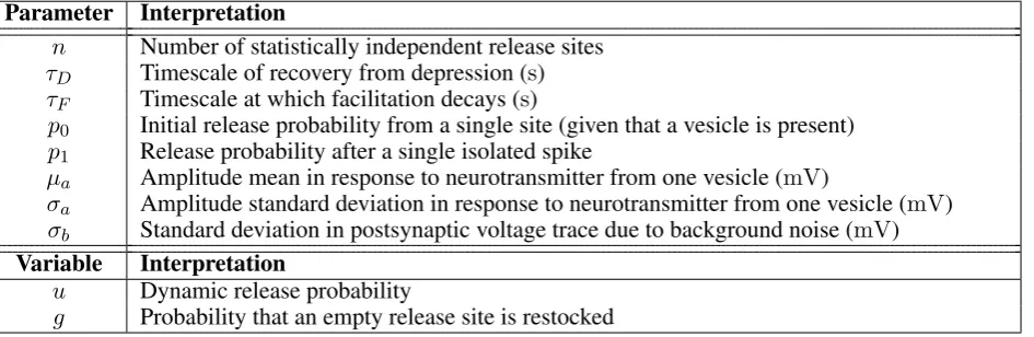
Parameter Interpretation
n Number of statistically independent release sites
τD Timescale of recovery from depression (s)
τF Timescale at which facilitation decays (s)
p0 Initial release probability from a single site (given that a vesicle is present) p1 Release probability after a single isolated spike
µa Amplitude mean in response to neurotransmitter from one vesicle (mV)
σa Amplitude standard deviation in response to neurotransmitter from one vesicle (mV)
σb Standard deviation in postsynaptic voltage trace due to background noise (mV)
Variable Interpretation
u Dynamic release probability
[image:6.595.52.525.75.229.2]g Probability that an empty release site is restocked
Table 1. Table of inferred parameters (top) and dynamic variables (bottom) used in the model of synaptic dynamics.
in occupancy before and after a presynaptic action potential can be straightforwardly derived to give 107
hxi⊕m =hxim−umhxim (2)
wherehximis the probability that a release site is occupied just before andhxi⊕mjust after themth spike. 108
Similarly, the probability of occupancy just before(m+ 1)th AP can be related to the occupancy just after 109
themth AP as 110
hxim+1= 1−(1− hxi⊕m)(1−gm) (3)
wheregmis the restock probability. For certain modelsgm can depend on the history of the presynaptic
111
APs. Together the recursion relations (2) and (3) give the occupancy probability for an arbitrary train 112
of presynaptic action potentials. The initial condition is typically taken as being hxi1 = 1, where all 113
release sites are stocked. These dynamics cover a range of models such as vesicle depression (Tsodyks 114
and Markram, 1997), depression with facilitation (Varela et al, 1997; Tsodyks et al, 1998; Fuhrmann et 115
al, 2002), frequency-dependent recovery (Fuhrmann et al, 2004) and and augmented recovery (Wang and 116
Kaczmarek, 1998; Hosoi et al, 2007). For an in-depth discussion, see Appendix A. 117
2.2 Illustrative synaptic model with depression and facilitation
118
To provide an example of the method we use a commonly used model that combines a depression 119
mechanism caused by vesicle release and a constant restock rate with a facilitation mechanism that models 120
the effect of increased release probability due to transient increases in calcium concentrations in the 121
presynaptic terminal (Varela et al, 1997; Tsodyks et al, 1998; Fuhrmann et al, 2002). The restock process is 122
Poissonian and has constant rate1/τD, whereτD is commonly referred to as the depression time constant;
123
therefore the restock probability required for equation (3) is simply 124
gm = 1−e−Tm/τD (4)
whereTm =tm+1−tmis the time between themth and(m+ 1)th APs. Letp0be the baseline value of 125
the probability of release, andp1be the facilitated release probability immediately after an isolated spike. 126
Letu(t)be the time-dependent release probability. In the absence of stimulus,u(t)decays back top0with 127
timescaleτF. The dynamics ofu(t)therefore obeys
128
du dt =
1
τF(p0−u) + (1−u)
p1−p0
1−p0
X
tm
δ(t−tm) (5)
where the(1−u)prefactor of the Delta functions prevents the probability going above unity. In this 129
setupu=p0if the previous spike was a long time ago, then on the arrival of a spike it jumps tou=p1. 130
Because it is a facilitation model we havep0 < p1<1. Note that this formulation of parameters allows the 131
facilitated release probabilityp1to be fixed independently of the initial release probabilityp0and maps 132
directly to the original quantal facilitating and depressing synaptic model of Fuhrmann et al (2002) with 133
p0 = USE and p1 = USE+ (1−USE)U1 using that paper’s notation. The values of u(t)just after the 134
mth and before the(m+ 1)th action potentials (u⊕mandum+1respectively) are defined by the following 135
recursion relations 136
u⊕m =um+ (1−um)
p1−p0
1−p0
and um+1 =p0+ (u⊕m−p0)e−Tm/τF (6)
where the initial conditions are thatu1=p0andu⊕1 =p1. This gives the release probability before each 137
presynaptic spike required for equation (2). The dynamics of the restock probabilitygare unaffected and 138
are given by equation (4). A special case of this model that has one less free parameter is when the release 139
probability doubles after an isolated spike and sop1 = 2p0(Tsodyks et al, 1998). 140
2.3 EPSP amplitude distribution
141
The post-synaptic amplitude statistics for single vesicle release of neurotransmitter is modelled by a 142
gamma distribution with meanµaand standard deviationσa. This is preferred over a normal distribution on
143
empirical grounds and ensures that amplitudes are always positive (Robinson, 1976; Hanse and Gustafsson, 144
2001; Bhumbra and Beato, 2013). However, it is reasonable to assume that background noise is normal 145
with standard deviationσb and is independent of EPSP amplitude. Note that this choice of amplitude
146
generation is identical to that described for isolated EPSPs in Bhumbra and Beato (2013). With this choice, 147
ifkvesicles release neurotransmitter from among thenpossible release sites, the observed EPSP amplitude 148
Ais written A = ψ+φ whereψ is the release-dependent component andφthe independent Gaussian 149
noise. Because ψ is the sum ofk individual quantal amplitudes, each of which are identically gamma 150
distributed, its distribution is also gamma-distributed with 151
P[ψ] = λ β
Γ(β)e
−λψψβ−1 where β =kµ2a σ2
a
and λ= µa σ2
a
. (7)
The distribution for the measured EPSP amplitudeA, givenk release events, is therefore a convolution 152
between the gamma and normally distributed components of the noise 153
P[A|k] = λ β
Γ(β) 1
(2πσb2)12
Z ∞
0
dye−λyyβ−1e
−(A−y)2
2σ2
b . (8)
An approach for numerically calculating this integral efficiently is provided in Appendix B. 154
2.4 Computational methods and code
155
An exhaustive grid-based derivation of the likelihood function for the depression-only model (see 156
Appendix) is just within the capabilities of easily accessible computers at the time of writing. However, 157
for more involved models with a greater number of parameters this becomes impracticable and a Markov 158
Chain Monte Carlo (MCMC) approach was used instead. Here priors are taken to be flat (uninformative) 159
for all parameters for illustrative reasons: more informative priors can be included as required. For the 160
MCMC implementation, parameter space is discretised into a grid and the sampler is initialised at a random 161
point consistent with any restrictions on the model parameters. Moves are proposed to each adjacent 162
grid point with equal probability and accepted or rejected based on the log-likelihood ratio of the current 163
and proposed points. Convergence of the sampler was examined by comparing the distributions resulting 164
from chains initiated in different locations. It is straightforward to extend this transparent implementation 165
in our code to include more sophisticated methods such as slice sampling. We provide MATLAB and 166
JULIA code for the Bayesian inference of synaptic parameters from measurements of synaptic amplitudes 167
using the Metropolis-Hastings sampling method (Metropolis et al, 1953; Hastings, 1970) described above 168
as part of the Supplementary Material. The code covers the major synaptic dynamics models including: 169
depression only, depression-facilitation, release-independent depression and frequency-dependent recovery. 170
The models are described in the Appendix. 171
2.5 Synthetic and experimental data
172
To test the model we used both artificial and experimental data sets. Synthetic data with known parameters 173
was generated from the synaptic-dynamics models and consisted of a series of stimulation times and 174
stochastically determined EPSP amplitudes. For experimental data sets the data analysed consisted of 175
EPSP amplitudes combined with their arrival times. The data, comprising paired whole-cell patch-clamp 176
recordings of layer-5 pyramidal neurons, was taken from a previous study (Kerr et al, 2013). Here data 177
obtained in control conditions and in the presence of100µMbath-applied adenosine was used. Presynaptic 178
cells were stimulated with square-pulse currents of5ms duration and magnitude sufficient to reliably 179
induce a single action potential without causing bursting. Stimulation consisted of10spikes at20−50Hz 180
with10s between traces ensuring sufficient time for full recovery and statistical independence for the next 181
sweep. For each presentation of the same presynaptic stimulus the amplitudes of the individual EPSPs 182
were extracted from the postsynaptic voltage trace using the voltage deconvolution method (Richardson 183
and Silberberg, 2008) providing a vector of 10 EPSP amplitudes. 184
3
RESULTS
In this section we first summarise the broad class of synaptic models our methodology applies to. We then 185
describe the nature of the computational problem involved in calculating exact correlated likelihoods. We 186
go on to show how the probability of observing a set of numbered release events for a chain of presynaptic 187
action potentials can be calculated using a Markovian property. By coupling this result to the miniature PSP 188
distribution, the full likelihood for an observed PSP amplitude train is then derived in the form of a matrix 189
multiplication. Finally, we demonstrate the method on both synthetic and experimental data, recovering the 190
shift in synaptic dynamics caused by the neuromodulator adenosine. 191
3.1 Synaptic models
192
We consider synaptic models that are quantal, stochastic and exhibit short-term plasticity. The synaptic-193
dynamics models featurensites where a vesicle can be present for release. If a vesicle is present just before 194
themth pulse then it is released with probabilityum. Between themth and(m+ 1)th pulses an empty
195
vesicle site can be restocked with probabilitygm. Both release (given a presynaptic AP) and restock events
196
are independent between release sites. The probabilities themselves are deterministic in that they depend 197
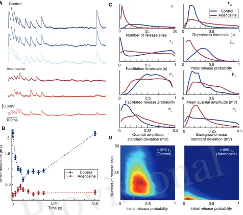
on the model parameters only and can be calculated in advance if the times of the action-potentialstm are
198
known. This formulation encompasses a very broad range of models of short-term plasticity. 199
When a vesicle is released, the size of the mini PSP it produces in the postsynaptic cell is modelled by 200
a gamma-distributed random variable (see Methods). The mini PSPs induced by different vesicles are 201
assumed to be independently identically distributed. The mean quantal amplitude isµaand the standard
202
deviation isσa. In addition there is a normally-distributed background noise with standard deviationσb
203
that is uncorrelated with EPSP amplitude. 204
For illustrative purposes we focus on a model of synaptic dynamics that features depression and facilitation 205
(Tsodyks and Markram, 1997; Fuhrmann et al, 2002), though other models for which computer code is 206
also provided are described in Appendix A. Activity reduces synaptic efficacy through vesicle depletion; 207
however, the build-up of Ca2+in a presynaptic terminal means that the probability of release given that a 208
vesicle is presentuis increased by presynaptic activity. Thus the response to sustained activity can involve 209
larger individual PSPs than the response to isolated spikes. Here, the model has a probabilityp0of release 210
for an isolated pulse; immediately after a presynaptic action potential the release probability increases to 211
p1. The release probabilityureturns to its initial valuep0 with a timescaleτF. Empty release sites are
212
restocked on a timescale ofτD. The model is fully defined in Methods and its parameters are summarised
213
in Table 1. 214
3.2 The nature of the computational problem
215
We now discuss the aim of Bayesian inference and the difficulties correlations cause in calculating the 216
necessary quantities. We consider that the data is in the form of a set of presynaptic action-potential times 217
t1,t2, · · ·,tM and post-synaptic amplitudesA1,A2 · · · AM. The aim of the inference procedure is to
218
calculate the probability densities of the parameters of the modelθ ={n, p0, p1, τD· · · }given the observed
219
presynaptic action potential times {t1,· · ·, tM} and postsynaptic amplitudes{A1,· · · AM}. Bayesian
220
inference utilizes the fact that the probability of a particular set of parameters being true, given some 221
observed data, is proportional to the probability of observing that data given that those parameters are 222
correct: 223
P(θ|AM, AM−1,· · · , A1)∝ L(AM, AM−1,· · ·, A1|θ). (9)
The termLon the right-hand side is referred to as the likelihood function. A-priori calculating the likelihood 224
appears computationally infeasible as naively it might be expected to grow exponentially with the number 225
of observed amplitudesM. For example, consider a case withnpossible release sites and a pair (M = 2of 226
presynaptic spikes. Then the likelihoodLis given by 227
L(A2, A1|θ) =
n X
k2=0 n X
k1=0
P[A2|k2]P[A1|k1]P[k2, k1] (10)
wherekm is the number of vesicles released by the mth spike. Because of the nested sums there are
228
(n+ 1)2additive terms in this expansion, and more generally the number of terms in the expansion grows 229
exponentially with the number of presynaptic action potentials∼(n+ 1)M. Written in this form it is clear 230
that the problem becomes computationally prohibitive for long trains of presynaptic spikes and this is 231
what makes calculation of the likelihood difficult for the complete model. The complexity arises from the 232
quantal part of the likelihoodP[k2, k1]; the individual amplitudesAm are dependent only on the number of
233
vesicleskm released by each action potential.
234
Note that if correlations are ignored and the approximation P(k2, k1) ' P(k2)P(k1) made, then the 235
likelihood factorises and reduces to a product form 236
L(A2, A1|θ) =
n X
k2=0
P[A2|k2]P[k2]
n X
k1=0
P[A1|k1]P[k1]
(11)
that is much more computationally tractable in that only2(n+ 1)terms are required. This approach was 237
taken by Costa et al (2013) and combined with an additional approximation that neglected quantal synaptic 238
components to focus on the mean effects of short-term plasticity. For the full probability density in which 239
correlations are retained, it is not possible to factorise the likelihood into a scalar product in this way. 240
However, we will show in the following sections that it is possible to use a Markovian property of this 241
likelihood to factorise the calculation into a matrix product. 242
3.3 Joint probability for serial release events
243
The quantal component of the likelihood is most problematic; to illustrate the method of tractably 244
calculating the full likelihood we will first consider the joint probability of paired release eventsP(k2, k1). 245
The generalisation to a train of many presynaptic action potentials is straightforward. Note that knowing the 246
number of release events at a particular action potential does not specify the state of the system; however, 247
knowing the number of occupied release sites before a spike does fully specify the state of system. This is 248
the Markovian property that makes likelihood calculation possible. We callym the number of available
249
vesicles present just before themth action potential. Note that the expected value ofym,E[ym] =nhxim,
250
wherehximobeys Eq. (2). Using this notation we can write the paired release probability in a more verbose 251
form 252
P(k2, k1) =
n X
y2=0 n X
y1=0
P(k2, y2, k1, y1). (12)
It is now possible to factorise the probability on the right-hand-side of the above equation. First we use the 253
product rule to expand as follows 254
P(k2, y2, k1, y1) = P(k2, y2, k1|y1)P(y1) (13)
= P(k2, y2|k1, y1)P(k1|y1)P(y1) (14)
= P(k2|y2, k1, y1)P(y2|k1, y1)P(k1|y1)P(y1) (15)
= P(k2|y2)P(y2|k1, y1)P(k1|y1)P(y1) (16)
where in the last step we have used the Markovian property of the occupancy variable. Note also that this is 255
an iterative procedure, in which we can factorise the joint probability starting with the first action potential 256
and then the second, that can be continued for joint probabilities that are comprised of an arbitrary number 257
of spikes. For example, for the case of three action potentials it is only necessary to multiply the two-spike 258
case byP(k3|y3)P(y3|k2, y2)with the generalisation to higher numbers of spike trains obvious. Inserting 259
the final result in equation (16) of this factorisation into equation (12) results in the following form for the 260
two-spike case 261
P(k2, k1) =
n X
y2=0 n X
y1=0
[P(k2|y2)] [P(y2|k1, y1)P(k1|y1)] [P(y1)] (17)
where the square parentheses have been used to isolate components depending onk2ork1or neither. This 262
form looks like an inner product and can be written in matrix-vector form (using bra-ket notation) as 263
P(k2, k1) = hl2|q1|r0i (18)
wherehl2|is a row vector dependent onk2,q1is an(n+ 1)by(n+ 1)matrix dependent onk1and|r0iis 264
a column vector that comprises the initial conditions. TypicallyP(y1) =δy1,nso that|r0ihas one non-zero
265
entry to indicate that the synapse is initially fully stocked with vesicles. Note also that the case of three 266
action potentials is straightforward 267
P(k3, k2, k1) =hl3|q2q1|r0i (19)
with obvious generalisation to higher numbers of spikes. The joint release probability can therefore be 268
reduced to matrix multiplication. The entries of the left row vector and matrices generally comprise two 269
forms. The first form is simply the number of release eventskmchosen from the occupancyym, using the
270
current probability of releaseum and is therefore binomial
271
P(km|ym) =
ym km
ukm
m (1−um)ym−km. (20)
The second form gives the occupancyym+1givenkmreleases from an occupancyym at the previous action
272
potential. This implies that there weren−ym+kmempty release sites just after themth pulse. We require
273
there to ben−ym+1empty sites just before the(m+ 1)th pulse which means thatym+1−ym+kmsites
274
were restocked. Letgmbe the restock probability of a single empty release site between timetm andtm+1 275
P(ym+1|km, ym) =
n−ym+km ym+1−ym+km
gmym+1−ym+km(1−gm)n−ym+1 (21)
where this quantity depends on the time between spikes for the synaptic-dynamics model (and all other 276
common synaptic models). 277
3.4 Joint probability for serial EPSP amplitudes
278
We can now use the factorised form for the serial quantal release events to calculate the full likelihood, 279
which is the joint probability density of seeing amplitudesA1andA2given the parameter set. 280
L(A2, A1|θ) =
X
y2 X
y1
n X
k2=0
P[A2|k2]P[k2|y2]
n X
k1=0
P[y2|k1, y1]P[A1|k1]P[k1|y1]
[P(y1)]. (22)
The probabilitiesP[A1|k1]andP[A2|k2]for the observed amplitudes given that a certain number of vesicles 281
were released are defined by Eq. (8). The form of Eq. (22) can again be interpreted as an inner product 282
n τD
τF p0
p1 µa
σa σb
Number of release sites Depression timescale (s)
Facilitation timescale (s) Initial release probability
Facilitated release probability Mean quantal amplitude (mV)
Quantal amplitude standard deviation (mV)
Background noise standard deviation (mV)
Pro
b
a
b
ili
ty
0 10 20 0 0.5 1
0 0.25 0.5 0 0.5 1
0 0.5 1 0 0.25 0.5
[image:12.595.180.491.74.446.2]0 0.1 0.2 0 0.1 0.2
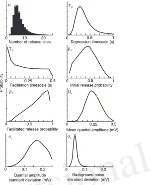
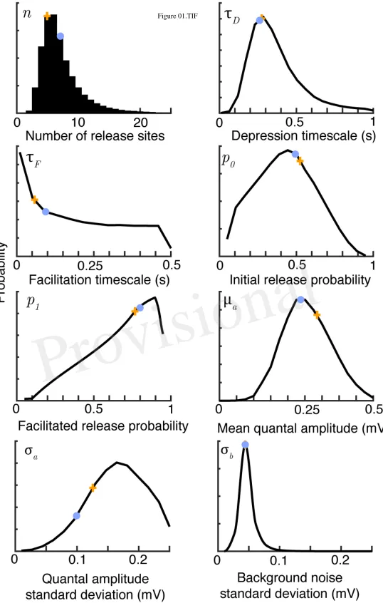
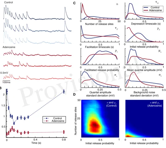
Figure 1. Bayesian inference provides parameter distributions from five sweeps of synthetic data comprising30regular spikes at30Hz. Marginal posterior distributions (black), maximuma-posteriori
estimates (orange crosses) and true parameter values (light blue dots) for the parameters of the facilitating synaptic model summarised in Table 1. Posteriors shown after 106 Metropolis-Hastings samples.The true values weren = 7,τD = 0.25s,τF = 0.1s,p0 = 0.6,p1 = 0.8,µa = 0.25mV,σa = 0.1mV and σb= 0.05mV.
which can be written in bra-ket notation 283
L(A2, A1|θ) =hL2|Q1|R0i (23)
wherehL2|is a row vector dependent onA2,Q1 is a matrix dependent onA1and|R0iis a column vector 284
with the initial configuration before the first action potential. This quantity is relatively straightforward to 285
compute and, importantly, does not grow exponentially in computational complexity for higher numbers of 286
action potentials. For example, for three spikes we have 287
L(A3, A2, A1|θ) = hL3|Q2Q1|R0i (24)
with the generalisation to higher numbers of presynaptic spikes straightforward. 288
3.5 Inferring quantal parameters from synthetic data
289
The methodology just described is first applied to synthetic data to test how well the correlated likelihood 290
function can recover quantal and dynamic parameters (Fig. 1). Here the synaptic-dynamics model is used 291
to generate sweeps of synthetic amplitude trains. For this model, the eight parameters to infer are the 292
release site numbern, initial release probabilityp0, facilitated release probability after an isolated spike 293
p1, depression timescaleτD, facilitation timescaleτF, mean quantal amplitudeµa, standard deviation in
294
quantal amplitudeσa, and standard deviation of background noiseσb.
295
Figure 1 shows marginal posterior distributions of these eight parameters given five simulated sweeps, 296
each of30regular spikes at30Hz. The posterior distributions reflect the true parameters well for all synaptic 297
parameters with the exception of the facilitation timescaleτF and quantal amplitude standard deviationσa.
298
These parameters have been observed to be hard to estimate in previous studies, with Costa et al (2013) 299
finding broad distributions forτF, and Bhumbra and Beato (2013) and Barri et al (2016) noting similar
300
uncertainties in their estimates of quantal variability. The correlated Bayesian method does not qualitatively 301
change these results, but makes the best use of available data to accurately estimate the uncertainty. The 302
posterior distributions narrow with more data, but it is also possible to change experimental protocols 303
to improve estimates. Costa et al (2013) note that when the stimulation process is Poisson, rather than 304
periodic, estimates of the time constantsτD andτF using their method are improved due to the broader
305
range of interspike intervals. This is equally true of the correlated Bayesian method. Estimates ofσa could
306
be improved by a very high stimulation rate that typically caused either 0 or 1 vesicles to release with each 307
spike. Note that with typical delays between sweeps of 15 seconds, collecting this dataset required just 308
over a minute of experimental time, giving a relatively sparse dataset that nevertheless still allows good 309
estimates of the underlying synaptic parameters. 310
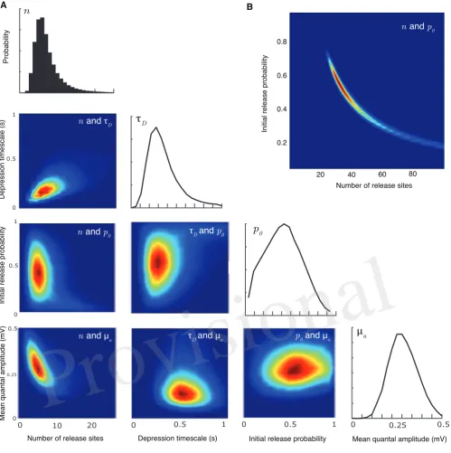
A major advantage of the Bayesian method over a maximum likelihood approach is that it can recover the 311
full distribution of parameters. This allows determination of the covariances between different parameters. 312
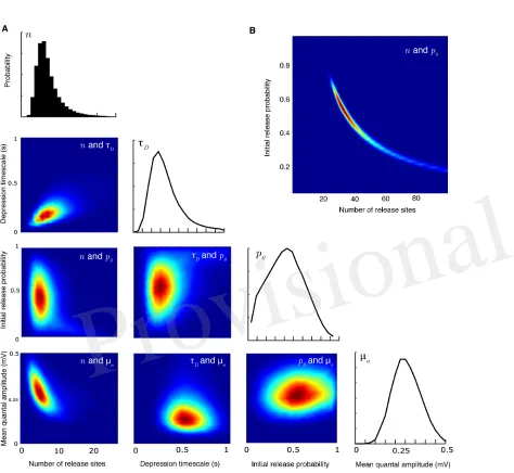
Figure 2 plots the joint posterior distributions of certain pairs of parameters (in total there are28possible 313
pairs for the synaptic-dynamics model considered here). Figure 2A shows the relationship between release 314
site numbern, depression timescaleτD, initial release probabilityp0, and mean quantal amplitudeµa. The
315
inverse relationship between estimates ofn andµa can be anticipated beause the mean EPSP size will
316
always depend on the product of these two quantities. Note in particular that the relationship between 317
release probability and bothnandτD has a characteristic curved shape that is not apparent from looking at 318
the individual marginal distributions. This is even more apparent (Fig. 2B) for larger values ofnthat can 319
be seen in some central synapses (Loebel et al, 2009, 2013). 320
3.6 Experiment: changing synaptic dynamics under adenosine application
321
The neuromodulator adenosine is implicated (Kerr et al, 2013) in the developmental shift from dominant 322
depression at juvenile synapses to weak facilitation at mature synapses (Reyes and Sakmann, 1999). 323
Adenosine acts viaA1receptors to ultimately reduce the probability of vesicle release (Dunwiddie and 324
Fredholm, 1989). Measurement of synaptic dynamics under control conditions and then during bath-325
application of adenosine therefore provides a convenient experimental protocol to test the inference method. 326
For the control case an initially depressing juvenile connection was stimulated40times with nine periodic 327
presynaptic spikes at40Hz and20Hz (see Fig. 3A) followed by a recovery spike, with the postsynaptic 328
response recorded. Adenosine (100µM) was then bath-applied to the slice (see Methods) and the stimulus 329
protocol repeated. 330
Figure 3A plots individual postsynaptic voltage traces before and after the application of adenosine; 331
Figure 3B shows the change in average EPSP size. The marginal maximum-likelihood estimates for the 332
depression timescaleτD and mean quantal amplitudeµa are similar between the control and adenosine
333
datasets (Fig 3C). However, the suppressive effect of adenosine on synaptic transmission is clearly visible 334
in the effective number of release sitesnand the initial release probabilityp0that drives the shift from 335
predominantly depressing to weakly facilitating synapses. It is also possible to examine the changes in 336
covariance between pairs of parameters inferred from the experimental data (Fig. 3D). Considering active 337
release sitesnand initial release probabilityp0together makes particularly apparent the shift in synaptic 338
transmission. 339
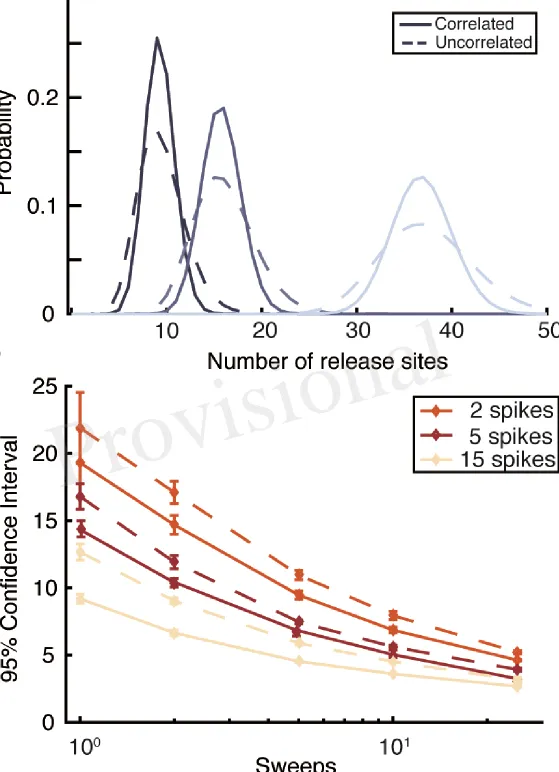
3.7 Comparison with methods that neglect serial correlations
340
Previous Bayesian inference methods have demonstrated that an uncorrelated likelihood function can 341
accurately infer the quantal (Bhumbra and Beato, 2013) and mean dynamic (Costa et al, 2013) parameters 342
of a synapse. It can therefore be asked under what conditions does the exact likelihood function, which 343
accounts for correlations, provide an improvement over existing methods. Synapses with low numbers of 344
release sitesn, high release probabilitiesu, or long depression timescalesτDhave the strongest correlations
345
between EPSPs. High release probabilitiesucan arise either at strongly depressing synapses, with a high 346
value ofp0, or facilitating synapses where the stimulation protocol causes large values ofu(t)to arise. In 347
addition to these, at least partly, physiological factors, the correlated likelihood function is superior in 348
conditions of sparse data. When only a few PSPs are available per sweep or, more importantly, only a 349
few sweeps are available correlations within a spike train are relatively more important. To quantify this, 350
we compared the full likelihood function described above with an approximated likelihood calculated by 351
ignoring correlations (calculated using forms like Eq. 11). The approximate likelihood did not account 352
for the observed previous PSP amplitudes within a sweep, only their distribution of probabilities given 353
by the model parameters and previous spike times. As expected, the uncorrelated likelihood function 354
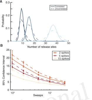
gave broader posterior distributions (Fig. 4A) with this effect diminishing as more data is added, either in 355
the form of more EPSPs per sweep or more independent sweeps (Fig. 4B). Overall, the exact likelihood 356
function that accounts for correlations provides superior inference on synaptic parameters. It is possible to 357
obtain accurate constraints on synaptic parameters with only a few sweeps, meaning that experiments could 358
capture a snapshot of synaptic properties in a small time window during protocols that change synaptic 359
properties on timescales of tens of seconds rather than tens of minutes. 360
4
DISCUSSION
We have presented a method for exactly and efficiently calculating the probability of a given train of PSP 361
amplitudes for dynamical synapses with the utility and robustness of the method demonstrated on synthetic 362
and experimental data. This method, presented earlier in Bird (2016) is equivalent to that simultaneously 363
and independently discovered by Barri et al (2016) in their expectation-maximization approach, and 364
represents a combination and extension of the recent work of Bhumbra and Beato (2013) on the exact 365
likehood of isolated events and Costa et al (2013) on the approximated likelihood of serial events. By 366
considering quantal and dynamic properties together, the method described accounts for information that is 367
necessarily neglected when each component is examined in isolation. The advance renders the calculation 368
of the likelihood required for Bayesian inference practical for a variety of models of short-term synaptic 369
plasticity. Moreover, unlike approaches that have relied on mean-variance analysis, it is applicable to 370
single-sweep experiments and so is suitable forin-vivoscenarios where presynaptic firing is uncontrolled, 371
but can be monitored. 372
The likelihood calculation that makes this inference possible is flexible and can be extended to a number 373
of common synaptic models, allowing for examination of augmented recovery (Wang and Kaczmarek, 374
1998; Hosoi et al, 2007), release-independent depression with frequency-dependent recovery (Fuhrmann et 375
al, 2004), and receptor desensitisation (Otis et al, 1996; Jones and Westbrook, 1996). Four such models are 376
described in Appendix A with associated computer code in the MATLAB and JULIA environments to be 377
found in the supplementary material. Another natural and straightforward extension of the methodology 378
presented here is to not assume that all sites are initially occupied but have the initial state of the system 379
as a parameter to be inferred. This scenario is relevant forin-vivoexperiments where there is no natural 380
break in the presynaptic activity: in this case the release site occupancy and state of the dynamic release 381
probability would be unknown. 382
CONFLICT OF INTEREST STATEMENT
The authors declare that the research was conducted in the absence of any commercial or financial 383
relationships that could be construed as a potential conflict of interest. 384
AUTHOR CONTRIBUTIONS
ADB and MJER wrote the paper, ADB and MJER derived the equations, ADB made the figures, ADB 385
wrote the MATLAB code and MJER wrote the JULIA code, MJW supervised experimental data collection. 386
FUNDING
We acknowledge funding through a Warwick Systems Biology Doctoral Training Centre fellowship to 387
Alex D. Bird, funded by the UK BBSRC funding agency (BBSRC Grant No. BB/G530233/1), and funding 388
to Magnus J. E. Richardson under BBSRC Grant No. BB/J015369/1. 389
ACKNOWLEDGMENTS
Data under adenosine was gathered by Dr Michael Kerr. Thanks to Dr Adam Newton (Warwick) and Dr 390
Peter Jedlicka (Frankfurt) for helpful comments on the manuscript. MJER thanks Dr Christophe Ladroue 391
for useful discussions. 392
SUPPLEMENTAL DATA
Supplementary Material comprises MATLAB and JULIA code to run Bayesian inference using the 393
depression (DEP), depression and facilitation (FAD), independent depression (RID) and release-394
independent depression with frequency-dependent recovery (FDR) synaptic models described, in the 395
Methods and Appendix A. 396
REFERENCES
Abbott LF. Synaptic depression and cortical gain control. Science 275, no. 5297: 221-224 397
doi:10.1126/science.275.5297.221, 1997. 398
Abbott L and W Regehr. Synaptic computation. Nature431: 796-803, 2004. 399
Barri A, Wang Y, Hansel D, and G Mongillo. Quantifying repetitive transmission at chemical synapses: a 400
generative-model approach. eNeuro, 2016. 401
Bekkers J. Quantal analysis of synaptic transmission in the central nervous system. Curr Opin Neurobiol
402
4: 360-365, 1994. 403
Bennett MR and T Florin. Statistical analysis of the release of acetylcholine at newly formed synapses in 404
striated muscle. J. Physiol238, no. 1: 93-107, 1974. 405
Bennett MR and JL Kearns. Statistics of transmitter release at nerve terminals. Prog. Neurobio.60, no. 6: 406
545-606, 2000. 407
Bird AD. Temporal and spatial factors affecting synaptic transmission in cortex. [PhD Thesis]. [Coventry 408
(UK)]: University of Warwick, 2016. 409
Bir`o A, Holderith N, and Z Nusser. Quantal size is independent of the release probability at hippocampal 410
excitatory synapses. J. Neurosci.25: 223-232, 2005. 411
Bhumbra GS and M Beato. Reliable evaluation of the quantal determinants of synaptic efficacy using 412
Bayesian analysis. J. Neurophysiol.109, no. 2: 603-620 doi:10.1152/jn.00528.2012, 2013. 413
Boyd IA and AR Martin. The end-plate potential in mammalian muscle. J. Physiol. 132, no. 1: 74 -91, 414
1956. 415
Br´emaud A, West D, and A Thomson. Binomial parameters differ across neocortical layers and with 416
different classes of connections in adult rat and cat neocortex. PNAS104: 1413414139, 2007. 417
Clements JD. Variance-mean analysis: a simple and reliable approach for investigating 418
synaptic transmission and modulation. J. Neurosci. Meth. 130, no. 2: 115-125 419
doi:10.1016/j.jneumeth.2003.09.019, 2003. 420
Costa RP, Sj¨ostr¨om PJ, and MCW van Rossum. Probabilistic inference of short-term synaptic plasticity in 421
neocortical microcircuits. Front. Comp. Neuro.7, no. 75 doi:10.3389/fncom.2013.00075, 2013. 422
del Castillo J, and B Katz. Quantal components of the end-plate potential. J. Physiol.124, no. 3: 560-573, 423
1954. 424
Dudel J and S Kuffler. Mechanism of facilitation at the crayfish neuromuscular junction. J. Physiol155: 425
530-42, 1961. 426
Dunwiddie TV and BB Fredholm. Adenosine A1 receptors inhibit adenylate cyclase activity and 427
neurotransmitter release and hyperpolarise pyramidal neurons in rat hippocampus. J. Pharmacol.
428
Exp. Ther.249(1): 31-7, 1989. 429
Eccles JC, Katz B, and Kuffler SW. Nature of the endplate potential in curarized muscle. J. Neurophysiol.
430
4, no. 5: 362-387, 1941. 431
Fatt P and B Katz. Spontaneous subthreshold activity at motor nerve endings. J. Physiol. 117, no. 1: 432
109-128, 1952. 433
Foster K and W Regehr. Variance-mean analysis in the presence of a rapid antagonist indicates vesicle 434
depletion underlies depression at the climbing fiber synapse. Neuron43, 119-131, 2004. 435
Franks K, Stevens C, and T Sejnowski. Independent sources of quantal variability at single glutamatergic 436
synapses. J. Neurosci.23 (8): 3186-3195, 2003. 437
Fuhrmann G, Segev I, Markram H, and Tsodyks M. Coding of temporal information by activity-dependent 438
synapses. J. Neurophysiol.87, no. 1: 140-148, doi:10.1152/jn.00258.2001, 2002. 439
Fuhrmann G, Cowan A, Segev I, Tsodyks M and Stricker C. Multiple mechanisms govern the 440
dynamics of depression at neocortical synapses of young rats. J. Physiol. 557, no. 2: 415-438, 441
doi:10.1113/jphysiol.2003.058107, 2004. 442
Furukawa T, Kuno M, and S Matsuura. Quantal analysis of a decremental response at hair cell-afferent 443
fibre synapses in the goldfish sacculus. J. Physiol.322: 181-195, 1982. 444
Hanse E and B Gustafsson. Quantal variability at glutamatergic synapses in area CA1 of the rat neonatal 445
hippocampus. J Physiol., 531, 2:467-480, 2001. 446
Hardingham NR, Read JCA, Trevelyan AJ, Nelson JC, Jack JJB, and NJ Bannister. Quantal analysis 447
reveals a functional correlation between presynaptic and postsynaptic efficacy in excitiatory connections 448
from rat neocortex. J. Neurosci., 30(4):1441-1451, doi:10.1523/jneurosci.3244-09.2010, 2010. 449
Hastings WK. Monte Carlo sampling methods using Markov chains and their applications. Biometrika57: 450
97-109, 1970. 451
Hosoi N, Sakaba T, and E Neher. Quantitative analysis of calcium-dependent vesicle recruitment and its 452
functional role at the Calyx of Held synapse. Journal of Neuroscience27(52): 14286-14298, 2007. 453
Jones MV and GL Westbrook. The impact of receptor desensitization on fast synaptic transmission. Trends
454
Neurosci19, no. 3: 96-101, 1996. 455
Kerr M, Wall M, and MJE Richardson. Adenosine a 1-receptor activation mediates the developmental 456
shift at Layer-5 pyramidal-cell synapses and is a determinant of mature synaptic strength. J. Physiol.
457
doi:10.1113/jphysiol.2012.244392., 2013. 458
Korn H, Triller A, Mallet A, and DS Faber. Fluctuating responses at a central synapse:nof binomial fit 459
predicts number of stained presynaptic boutons. Science213, no. 4510: 898-901, 1981. 460
Kuno M. Quantal components of excitatory synaptic potentials in spinal motoneurones. J. Physiol.175: 461
81-99 doi:10.1016/j.ceca.2007.02.008, 1964. 462
Kuno M. Quantum aspects of central and ganglionic synaptic transmission in vertebrates. Physiol. Rev.51, 463
no. 4: 647-678, 1971. 464
Kuno M and JN Weakly. Quantal components of the inhibitory synaptic potential in spinal mononeurones 465
of the cat. J. Physiol.224, no. 2: 287-303, 1972. 466
Lefort S, Tomm C, Sarria JCF, and CCH Petersen. The excitatory neuronal network of the C2 barrel column 467
in mouse primary somatosensory cortex. Neuron61, no. 2: 301-316 doi:10.1016/j.neuron.2008.12.020, 468
2009. 469
Liley AW. The quantal components of the mammalian end-plate potential. J. Physiol.133, no. 3: 571-587, 470
1956. 471
Loebel A, Silberberg G, Helbig D, Markram H, Tsodyks M, and MJE Richardson. Multiquantal release 472
underlies the distribution of synaptic efficacies in the neocortex. Front. Comp. Neuro. 3, no. 27 473
doi:10.3389/neuro.10.027.2009, 2009. 474
Loebel A, Le B`e JV, Richardson MJ, Markram H, and AV Herz. Matched pre- and post-475
synaptic changes underlie synaptic plasticity over long time scales. J. Neurosci. 33(15):6257-66 476
doi:10.1523/JNEUROSCI.3740-12.2013, 2013. 477
McGuinness L, Taylor C, Taylor RDT, Yau C, Langenhan T, Hart ML, Christian H, Tynan PW, Donnelly 478
P, and NJ Emptage. Presynaptic NMDARs in the hippocampus facilitate transmitter release at theta 479
frequency. Neuron68, no. 6: 1109-1127 doi:10.1016/j.neuron.2010.11.023, 2010. 480
Metropolis N, Rosenbluth AW, Rosenbluth MN, Teller AH, and E Teller. Equation of state calculations by 481
fast computing machines. J. Chem. Phys.21:1087-1092, 1953. 482
Mongillo G, Barak O, and M Tsodyks. Synaptic theory of working memory. Science319: 1543-1546, 483
2008. 484
Otis T, Zhang S, and LO Trussel. Direct measurement of AMPA receptor desensitization induced by 485
glutamatergic synaptic transmission. J. Neurosci.16, no. 23: 7496-7504, 1996. 486
Reyes A and B Sakmann. Developmental switch in the short-term modification of unitary EPSPs evoked in 487
layer 2/3 and layer 5 pyramidal neurons of rat neocortex. J. Neurosci., 19:3827-3835, 1999. 488
Richardson MJE and G Silberberg. Measurement and analysis of postsynaptic potentials using a novel 489
voltage-deconvolution method. J. Neurophysiol.99, no. 2: 1020-1031 doi:10.1152/jn.00942.2007, 2008. 490
Robinson J. Estimation of parameters for a model of transmitter release at synapses. Biometrics, 32:61-68, 491
1976. 492
Silver R, Momiyama A, and S Cull-Candy. Locus of frequency- dependent depression identified with 493
multiple-probability fluctuation analysis at rat climbing fibre-Purkinje cell synapses. J. Physiol 510:881-494
902, 1998. 495
Silver R. Estimation of nonuniform quantal parameters with multiple-probability fluctuation 496
analysis: theory, application and limitations. J. Neurolsci. Meth. 130, no. 2: 127-141 497
doi:10.1016/j.jneumeth.2003.09.030, 2003. 498
Song S, Sj¨ostr¨om PJ, Reigl M, Nelson S, and DB Chklovskii. Highly nonrandom features of synaptic 499
connectivity in local cortical circuits. PLoS Biology3, no. 3:68 doi:10.1371/journal.pbio.0030068.st001, 500
2005. 501
Stein RB. A theoretical analysis of neuronal variability. Biophys. J.5, no. 2: 173-194 doi:10.1016/S0006-502
3495(65)86709-1, 1965. 503
Thomson AM, Deuchars J, and DC West. Large, deep layer pyramid-pyramid single axon EPSPs in slices 504
of rat motor cortex display paired pulse and frequency-dependent depression, mediated presynaptically 505
and self-facilitation, mediated postsynaptically. J. Neurophysiol.70, no. 6: 2354-2369, 1993. 506
Tsodyks MV and H Markram. The neural code between neocortical pyramidal neurons depends on 507
neurotransmitter release probability. PNAS94, no. 2: 719-723 doi:10.2307/41270, 1997. 508
Tsodyks MV, Pawelzik K, and H Markram. Neural networks with dynamic synapses. Neural Comp.10, 509
no. 4: 821-835, 1998. 510
Turner D and M West. Bayesian analysis of mixtures applied to post-synaptic potential fluctuations. J.
511
Neurosci. Meth.47:1-21, 1993. 512
Varela JA, Sen K, Gibson J, Fost J, Abbott LF, and SB Nelson. A quantitative description of short-term 513
plasticity at excitatory synapses in layer 2/3 of rat primary visual cortex. J. Neurosci. 17, no. 20: 514
7926-7940, 1997. 515
Wang L and L Kaczmarek. High-frequency firing helps replenish the readily releasable pool of synaptic 516
vesicles. Nature, 394: 384-388, 1998. 517
Zucker RS and WG Regehr. Short-term synaptic plasticity. Annu. Rev. Physiol
518
doi:10.1146/annurev.physiol.64.092501.114547, 64: 355-405, 2002. 519
APPENDIX A. EXTENSION TO OTHER SYNAPTIC MODELS
The likelihood calculation that was illustrated in the main text for a model with depression and facilitation 520
can be straightforwardly adapted to other commonly used models of synaptic dynamics. These comprise 521
models in which the restock probability gm between presynaptic action potentials m and m+ 1 and
522
probability of release at the arrival of themth action potentialumdepends only on the pattern of presynaptic
523
activity. As part of the supplementary material we provide computer code for four such models, which are 524
now described below with the synaptic parameters and dynamic variables tabulated in Table 2. 525
(i) Depression only - DEP model
526
This is perhaps the simplest model of short-term synaptic plasticity and features only vesicle depletion and 527
restock (Tsodyks and Markram, 1997; Fuhrmann et al, 2002). The occupation of a single release site is 528
governed by the stochastic differentional equation (1). The mean-occupancy recursion relations for the 529
model are given by equations (2) and (3) with a constant release probabilityum =p0. The Poissonian 530
restock of empty release sites occurs at a constant rate1/τD and so in this case the restock probabilitygm
531
is given by Eq. (4). 532
(ii) Depression and facilitation - DAF model
533
This is the model described in the main text (Varela et al, 1997; Tsodyks et al, 1998; Fuhrmann et al, 2002) 534
applies to facilitating synapses. The probability of restock is defined by Eq. (4) and the probability of 535
releaseum is given by recursion equations (6).
536
(iii) Release-independent depression - RID model
537
This model was introduced (Fuhrmann et al, 2004) for synapses that do not display facilitation and 538
considers a different form of depression which is uncorrelated with the preceding EPSP amplitudes. 539
Release-independent depression is a reduction in release probabilityumcaused by spiking activity which
540
decays on a timescale τI0 (it can be thought of as a kind of anti-facilitation). The release probability
541
immediately after an isolated pulse is again called p1 but in contrast to facilitation p1 < p0. In this 542
formalism the release probabilityu(t)obeys 543
du dt =
p0−u
τI0
− u p0
(p0−p1)
X
tm
δ(t−tm) (25)
wheretmare the times of the presynaptic action-potentials. The values ofu(t)just after themth and before
544
the(m+ 1)th action potentials (u⊕m andum+1respectively) are defined by the following recursion relations 545
u⊕m =um−um
p0−p1
p0
and um+1 =p0+ (u⊕m−p0)e−Tm/τI0. (26)
The restock probabilitygmis given by equation (4) and is common to the previous two models.
546
(iv) Release-independent depression with frequency dependent recovery - FDR model
547
The recovery from release-independent depression is often seen to be frequency dependent (Fuhrmann et 548
al, 2004). To account for this the timescaleτI(t)is now a dynamic variable with initial valueτI0, has a
549
magnitude after an isolated spike ofτI1 and decay timescaleςI. The relevant equations are now
550
du
dt =
p0−u
τI
− u p0
(p0−p1)
X
tm
δ(t−tm) (27)
dτI
dt =
τI0−τI
ςI
− τI τI0
(τI0 −τI1) X
tm
δ(t−tm) (28)
The dynamicRIDrecovery timescale τI(t)obeys Eq. (28). The values of τI(t) just after the mth and
551
before the(m+ 1)th action potentials (τIm⊕ andτIm+1respectively) are defined by the following recursion 552
relations 553
τIm⊕ =τIm−τIm
τI0−τI1
τI0
and τIm+1=τI0+ (τ
⊕
Im−τI0)e
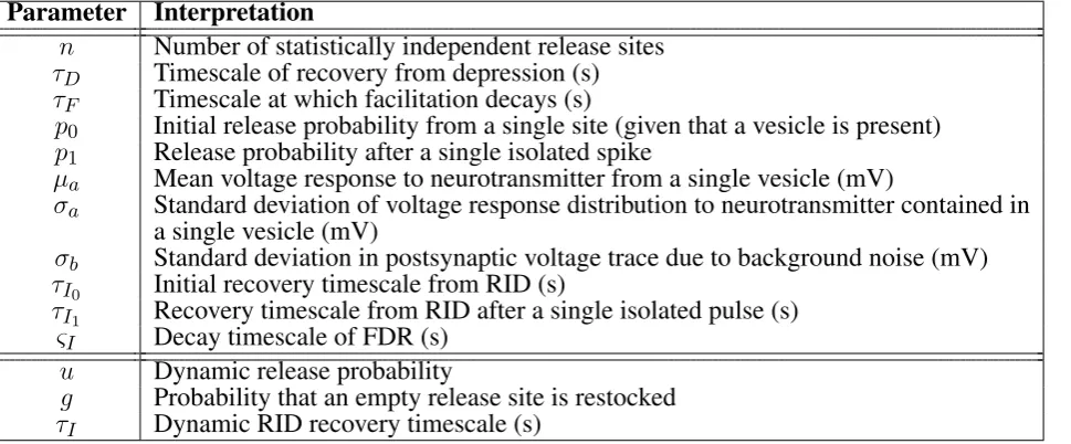
Parameter Interpretation
n Number of statistically independent release sites τD Timescale of recovery from depression (s) τF Timescale at which facilitation decays (s)
p0 Initial release probability from a single site (given that a vesicle is present)
p1 Release probability after a single isolated spike
µa Mean voltage response to neurotransmitter from a single vesicle (mV)
σa Standard deviation of voltage response distribution to neurotransmitter contained in
a single vesicle (mV)
σb Standard deviation in postsynaptic voltage trace due to background noise (mV) τI0 Initial recovery timescale from RID (s)
τI1 Recovery timescale from RID after a single isolated pulse (s) ςI Decay timescale of FDR (s)
u Dynamic release probability
[image:20.595.51.536.75.276.2]g Probability that an empty release site is restocked τI Dynamic RID recovery timescale (s)
Table 2. Extended table of inferred parameters (top) and dynamic variables (bottom) used in the synaptic models discussed in Appendix A.
The release probabilityu(t)obeys Eq. (27) and can also be defined recursively, with um+1the release 554
probability at the(m+ 1)th spike at timetm+1given by 555
um+1 =p0+
u⊕m−p0 τIm⊕ ςI τI0
τIm⊕ −τI0
1−e
Tm ςI
ςI τI0
(30)
whereu⊕m =um−um
p0−p1 p0
is the release probability immediately following themth spike. 556
APPENDIX B - THE LIKELIHOOD CONVOLUTION INTEGRAL
The convolution integral for the amplitude distribution Eq. (8) must be computed a large number of times. 557
There are two difficulties in doing this efficiently: (i) evaluating a gamma distribution for large shape 558
parameters and (ii) finding reasonable bounds for the range of integration. 559
Evaluating a gamma distribution
560
Whenµa σa, the argument of the gamma function in the denominator of Eq. (8) can grow very large in
561
order to normalise the distribution. To avoid issues with this, we note that Stirling’s approximation allows 562
evaluation of the gamma function with large arguments 563
Γ(z)≈
r 2π
z
z e
z
1 + 1 12z +
1 288z2 −
139 51840z3 −
571 2488320z4
and defineκ(z)such that 564
κ(z) = 1 Γ(z)
r 2π z z e z (32) ≈ 1 + 1
12z + 1 288z2 −
139 51840z3 −
571 2488320z4
−1
. (33)
For small values ofz,κ(z)can be evaluated exactly, whereas for larger arguments this approximation is 565
used. 566
Bounding the range of integration
567
The second difficulty involves finding bounds for the range of integration in Eq. (8). Usingκas above, the 568
integralI(k, Ai, µa, σa, σb)
569
I =
µa σ2a
k
µ2a σ2a
Γ(kµ2a σ2a)
1 √
2πσb
R∞
0 s
kµ 2
a σa2−1e−
µas σa2 e
−(Ai−s)2
2σ2
b dz (34)
can be rewritten as 570
I = κ(α−1)β ασα−1
b 2παα−1/2e−α e
−Aiβ+
(σbβ)2 2
Z ∞
0
zθe−(z−22φ) 2
dz (35)
where the variable of integration has been rescaled such thatz = σs
b, the gamma distribution parameters 571
are grouped so thatα = kµ2a
σa2 andβ =
µa
σa2, and we have introducedθ =k
µ2a
σ2a −1and φ =
Ai
σb −
µaσb
σ2a to 572
reduce the integral to two parameters. The integrand has a maximum atz =z∗wherez∗ =φ+
p
φ2+θ. 573
We seek to compute the integral over a range where the integrand takes a non-negligible proportion of its 574
value atz∗. Iff(z) =zθe−
(z−2φ) 2
2
is the integrand, we find the interval wheref(z)> e−10f(z∗)using the
575
Newton-Raphson method. The integral can then be accurately evaluated over this region. 576
n
τD
p0
µa
Initial release probability Mean quantal amplitude (mV) Depression timescale (s)
Number of release sites
40 60 80
20
B
0.8
0.6
0.4
0.2
Number of release sites
In
it
ia
l
re
le
a
se
p
ro
b
a
b
ili
ty
A
n andp0
n andτD
n andμa
τD andp0
τD andμa p0andμa
n andp0
Pro
b
a
b
ili
ty
D
e
p
re
ssi
o
n
t
ime
sca
le
(s)
In
it
ia
l
re
le
a
se
p
ro
b
a
b
ili
ty
Me
a
n
q
u
a
n
ta
l
a
mp
lit
u
d
e
[image:22.595.47.547.76.578.2](mV)
Figure 2. Joint parameter estimates for the synaptic-dynamics model.APairwise and individual posterior marginals for release-site numbern, depression timescaleτD, initial release probabilityp0, and mean
quantal amplitudeµa. True parameter values and data are the same as Fig. 1. Colourbars for the values of
the posterior distributions are not shown; the relative differences in value show the shape and sharpness of the pairwise posteriors for each pair of parameters.BPairwise posterior marginal for release site numbern and initial release probabilityp0for a case where the true values weren = 35andp0 = 0.50showing a
strong anticorrelation. All posteriors shown after106Metropolis-Hastings samples.
100ms 0.5mV
Adenosine Control
2
1 1.5
0.5
Control Adenosine
0 0.4 0.8
Time (s)
EPSP
a
m
p
lit
u
d
e
(mV)
A
n τD
τF p0
p1 µa
σa σb
Number of release sites Depression timescale (s)
Facilitation timescale (s) Initial release probability
Facilitated release probability Mean quantal amplitude (mV)
Quantal amplitude standard deviation (mV)
Background noise standard deviation (mV)
0 25 50 0 0.5 1
0 0.5 1 0 0.5 1
0 0.5 1 0 0.5 1
0 0.25 0.5 0 0.25 0.5
Control Adenosine
n and p0 (Control)
n and p0 (Adenosine)
Initial release probability
0 0.5 1
Initial release probability
0 0.5 1
N
u
mb
e
r
o
f
re
le
a
se
si
te
s
25 50 B
C
[image:23.595.44.521.75.496.2]D
Figure 3. Bayesian inference captures the shift in synaptic dynamics under application of adenosine.A
Individual postsynaptic voltage traces under control (top) and adenosine (bottom) conditions.B Mean EPSP size for each spike in the stimulation protocol under control (blue) and adenosine (red) conditions. Bars show standard error.CMarginal posterior distributions for the parameters of the synaptic model in the control (blue) and adenosine (red) conditions.DPairwise posterior marginals for number of active release sitesnand initial release probabilityp0before (left) and after (right) application of adenosine. Posteriors
shown after5×106Metropolis-Hastings samples.
Number of release sites 0
0.1 0.2 0.3
Pro
b
a
b
ili
ty
Correlated Uncorrelated
Sweeps 0
5 10 15 20 25
9
5
%
C
o
n
fi
d
e
n
ce
I
n
te
rva
l 5 spikes2 spikes
15 spikes
A
B 10 20 30 40 50
[image:24.595.179.493.77.421.2]100 101