from bags of words to strings of words
Luc Schoot Uiterkamp
Supervisor:
Prof. Dr. Frank van der Velde
Second reader: Dr. Martin Schmettow
Cognitive Psychology and Ergonomics Faculty of behavioural and manage-ment sciences, University of Twente, P.O. Box 217, 7500 AE Enschede, The Netherlands
Master thesis, august 2019
01100110 01110010 01101111 01101101 00100000 01100010 01100001 01100111 01110011 00100000 01101111 01100110 00100000 01110111 01101111 01110010 01100100 01110011 00100000
Abstract
Natural language as we use it daily is often ambiguous, as words and sentences can
have different meanings depending on the context in which they are used. Humans
derive meaning from words using contextual information and word relations, which is
something we do automatically. Most computer algorithms rely on rules and an absence
of ambiguity to process information. Since the contextual cues we use to communicate
meaning cannot be readily captured in rules, such algorithms cannot reliably interpret
natural language. Machine learning algorithms enable computers to model in some way
what human-made texts mean. In this thesis, a machine learning algorithm is used
to estimate whether reviews of movies and tv shows taken from imdb give a positive
or negative appraisal of their respective movie or show. The reviews are represented
as vectors of numbers to enable the machine learning algorithm to process the text.
The method of representing these reviews that is currently standard, the ‘bag of words’
representation, represents the reviews in terms of how frequently each word in a predefined
word list occurs in each review. The original arrangement of the words in the review is
lost, as the representation is ordered in terms of the predefined word list. This limits the
use of contextual information and word relations, which forms a barrier to interpreting
what was meant. An alternative to the bag of words text representation is presented,
which enables the original arrangement of the words in a text to be used. The alternative
‘string of words’ representation represents texts in terms of the original words of a text,
in the original order. This differs from the bag of words representation, which represents
the text in the order of the words that are known to the model. To find out if a machine
learning classifier can be improved by the string of words representation, it is tested
against the bag of words representation in a neural network that classifies movie and tv
show reviews into two categories: positive and negative reviews. For both conditions in
the comparison between word representations, the same neural network layers were used
as a basis for the machine learning model.
To compare the two representations, performance and time measures were taken. The
performance was measured as the MCC value, a combined confusion matrix measure, of
the classifier model that was yielded using that representation. The impact of
representa-tion length of the string of words representarepresenta-tion and the lengths of the classified reviews
The string of words representation outperforms the bag of words in time measures as well
as performance measures but does come with its own limitations. The string of words
representation performs best with texts that deviate little in length from the training
texts and offers an advantage over the bag of words representation only if the text length
is shorter than the number of words known to a machine learning model.
Contents
Abstract 2
1 Introduction 7
2 Sentiment analysis 8
3 Machine learning 10
3.1 Vocabulary . . . 11
3.2 Neural networks . . . 13
3.3 Feature extraction . . . 14
3.4 Bag of Words . . . 14
3.4.1 Loss of word arrangement . . . 15
3.4.2 Sparsity of data . . . 16
3.5 String of words . . . 18
3.5.1 Advantages of SOW . . . 20
4 Neural network 22 4.1 Overview . . . 22
4.2 Importing and normalization . . . 24
4.3 Processing . . . 27
4.4 Neural network layers . . . 29
4.4.1 Embedding . . . 30
4.4.2 LSTM . . . 31
4.4.3 Fully connected . . . 34
4.4.4 Regression . . . 35
4.4.5 Updating weights . . . 35
5 Research 35 5.1 Hypotheses . . . 35
5.2 Dataset . . . 36
5.3 Model implementation . . . 37
5.3.1 Training variables . . . 37
5.3.3 Design . . . 39
5.4 Data visualization . . . 39
5.5 Model comparison methods . . . 40
5.6 Comparison of measures . . . 41
5.7 Exploratory analysis: Truncation length and text length . . . 42
6 Results 43 6.1 Data properties . . . 43
6.1.1 Review lengths . . . 43
6.1.2 Part of speech tags . . . 43
6.2 Analysis results . . . 44
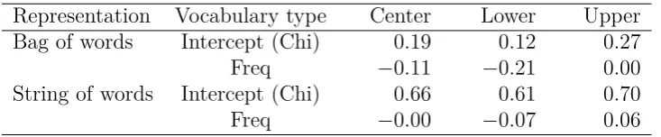
6.2.1 Vocabulary type . . . 44
6.2.2 MCC values . . . 45
6.2.3 Time measures . . . 45
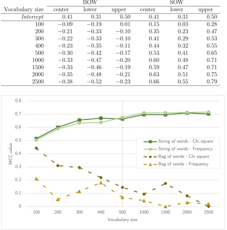
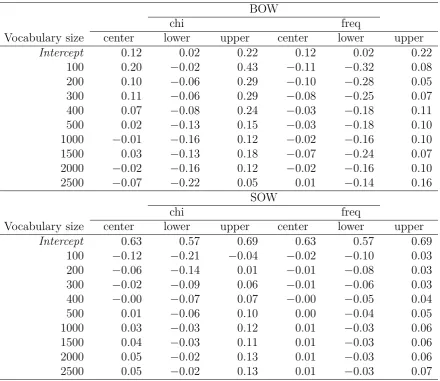
6.3 Truncation length and text length . . . 47
7 Discussion 51 7.1 Vocabulary types . . . 51
7.2 BOW vs SOW . . . 52
7.3 Durations . . . 52
7.4 Model performance . . . 53
7.5 Truncation length . . . 55
7.6 Assumptions . . . 55
7.7 Limitations . . . 56
7.7.1 Limitations of sentiment analysis in general . . . 56
7.7.2 Limitations to this study . . . 56
7.7.3 Limitations of the string of words model . . . 57
7.8 Future research . . . 57
8 Summary 59 8.1 Conclusions . . . 59
Appendix A Background reading on probabilistic classifiers 64
A.1 Generative classifiers . . . 64
A.1.1 Bayesian classifiers . . . 64
A.1.2 Training Bayesian classifiers . . . 65
A.2 Discriminative classifiers . . . 67
A.2.1 Logistic regression classifier . . . 67
A.2.2 Training logistic regression classifiers . . . 68
Appendix B Other word representation structures 70 B.2 Tree-like structures . . . 70
B.3 N-grams and n-grams as bag of words . . . 71
B.4 N-grams as feature vector . . . 72
Appendix C Worked out example of the model 74
Appendix D R markdown 75
Appendix E List of unused reviews 80
1 Introduction
Natural language is language as we use it in our day-to-day lives. It is often ambiguous;
words and sentences can have different meanings, dependent on the context in which
they are used (Jurafsky & Martin, 2017). Most humans have very little trouble with
disambiguating natural language and interpreting it. We achieve this by using contextual
cues and previously learned information.
This can be very simple: the sentence “I saw her duck” can be interpreted in two ways. Firstly, someone might have seen a duck belonging to a girl or woman or, secondly,
someone might have seen a girl or woman bend or crouch down. If a person would be
asked what this sentence meant, they would use contextual cues to figure out the meaning.
If the girl or woman in question was about to be hit by, say, a paper airplane, this would
indicate that she was crouching down. Contrarily, if the girl or woman is known to own
a duck, the likelihood of the first meaning of the sentence would increase.
The use of contextual cues and previous knowledge to disambiguate sentences such as “I
saw her duck” is something people do automatically. We learn language by doing, and
get better at it by coming into contact with language around us. Even though we do
learn some explicit grammar rules, intuition plays a big part in our language processing.
Our procedural knowledge of language is very high, it is not difficult to recognize the two
meanings of “I saw her duck” but it is more difficult to explain exactly why there are two
meanings, and why one would be more likely than another. It requires more than just
the grammatical rules of our language to do this.
Unlike humans, computers rely on rules and unambiguous information to process an
input. Although our language is structured, in a grammatical sense, what is meant by a
sentence may not be obvious from the grammatical rules alone, as could be seen in the
duck example. For this reason, computer programs that are solely based on rules have
a limited ability of determining the correct interpretation of a certain piece of natural
language. Hence, to enable computer programs to extract meaning from natural language,
algorithms that are not solely rule based are required.
In this thesis, the automated interpretation of one aspect of the meaning of a piece of
natural language called ‘sentiment analysis’ is investigated. Reviews from movies and tv
shows taken from imdb1 are classified as either positive or negative reviews, based on the
content of the review. A neural network based machine learning algorithm will be used
to perform the sentiment analysis in this study. To enable the reviews to be processed by
the machine learning model, they are represented as a vector. This is often done using
the so called ‘bag of words’ method, with which it is not possible evaluate words in their
original arrangement. This hinders the use of context to determine the meaning of a
piece of text which is problematic because, as we have seen in the duck-example, context
is very important for a correct interpretation.
An alternative to the bag of words representation is presented and tested. This ‘string
of words’ representation is developed to operate more similarly to how humans process
language and to improve the ability of machine learning models to take context into
account.
The goal of the thesis is to find out which of the two word representations performs
better in a number of conditions. Performance is measured as the ratio of true versus
false predictions made by a machine learning model. The machine learning model will be
tested with both the bag of words and string of words representations, and performance
measures will be compared using a Bayesian linear model. Time measures are also taken
into consideration and divided into preparation time, training time and total time.
In section 2 some background is given on the main topic of this thesis, which is sentiment
analysis. Machine learning, described in section 3, will be used for this. The Bag of Words
(BOW) word representation is explained in section 3.4 and some problems are identified.
Previous solutions to these problems are identified in section B and the String of Words
(SOW) solution is presented in section 3.5. Some examples of traditional classification
algorithms are given in section A to give a background on machine learning classifiers,
which relate to the machine learning model that stands at the core of this thesis, which
is described in sections 4.1 and 4.4. The methods for evaluating the word representations
are presented in section 5, the results in section 6.
2 Sentiment analysis
The “I saw her duck” example is a fairly simple and straightforward piece of natural
language, where the correct interpretation out of two options needed to be determined.
This is an example of language disambiguation: there are multiple interpretations for a
One step further in extracting meaning from a text is ‘sentiment analysis’, the extraction
of the author’s feeling towards what is described in the text. Sentiment analysis tries to
capture what an author is trying to get across using the natural language as a medium.
This analysis can be done on multiple levels of abstraction, from identifying the emotional
connotation of a sentence - for example answering the question ‘does the author feel happy
or sad regarding the subject of the text?’ - to identifying whether the stance of an author
regarding the subject of their text is positive or negative.
Sentiment analysis can be seen as an estimation task, in which sentiment can be estimated
on a continuous scale ranging from for example positive to negative, or as a classification
task, in which a text is classified as either ‘positive’ or ‘negative’. In this thesis, a sentiment
analysis task is performed but is limited to classifying stance toward the subject of a text
into one of two classes: positive or negative. This analysis is carried out on reviews of
movies and tv shows, generated by imdb users. The dataset used was compiled by Maas
et al. (2011) and made available for research in machine learning. The reviews have been
selected by Maas et al. (2011) to represent extremes of the scale, only distinctly positive
or distinctly negative reviews are used. Reviews were considered positive if they had a
rating of seven out of ten or higher and negative if they had a rating of four out of ten
or lower. Reviews with scores between four and seven were not included in the dataset.
Because of this dichotomy in the dataset, a binary classification task was performed
instead of a continuous scaling. Figure 1 shows an example of a positive review (1a) and
a negative review (1b) as they are used in this thesis.
It is often difficult for us to make explicit why we interpret language in a certain way,
even for ourselves. Humans process language in a procedural manner, not in an explicitly
descriptive manner. This means that we have the ability to correctly apply language rules
and interpret meaning in language correctly, but that it is difficult to specify exactly how
we come to the correct conclusions. In the examples of movie reviews in figure 1 it is quite
easy to determine in which class - positive or negative - both reviews belong. When trying
to point out why, the positive and negative words in both reviews might be mentioned.
However, looking at what words are used in both reviews might be misleading. The
positive review features words like ‘coaxed’, ‘reluctant’ and ‘wrong’, seemingly negative
words. The negative review on the other hand features words like ‘legendary’, ‘lovely’ and
(a) Positive review example
I went and saw this movie last night after being coaxed to by a few friends of mine. I’ll admit that I was reluctant to see it because from what I knew of Ashton Kutcher he was only able to do comedy. I was wrong. Kutcher played the character of Jake Fischer very well, and Kevin Costner played Ben Randall with such professionalism. The sign of a good movie is that it can toy with our emotions. This one did exactly that. The entire theater (which was sold out) was overcome by laughter during the first half of the movie, and were moved to tears during the second half. While exiting the theater I not only saw many women in tears, but many full grown men as well, trying desperately not to let anyone see them crying. This movie was great, and I suggest that you go see it before you judge.
(b) Negative review example
Blake Edwards’ legendary fiasco, begins to seem pointless after just 10 minutes. A combination of The Eagle Has Landed, Star!, Oh! What a Lovely War!, and Edwards’ Pink Panther films, Darling Lili never engages the viewer; the aerial sequences, the musical numbers, the romance, the comedy, and the espionage are all ho hum. At what point is the viewer supposed to give a damn? This disaster wavers in tone, never decides what it wants to be, and apparently thinks it’s a spoof, but it’s pathetically and grindingly square. Old fashioned in the worst sense, audiences understandably stayed away in droves. It’s awful. James Garner would have been a vast improvement over Hudson who is just cardboard, and he doesn’t connect with Andrews and vice versa. And both Andrews and Hudson don’t seem to have been let in on the joke and perform with a miscalculated earnestness. Blake Edwards’ SOB isn’t much more than OK, but it’s the only good that ever came out of Darling Lili. The expensive and professional look of much of Darling Lili, only make what it’s all lavished on even more difficult to bear. To quote Paramount chief Robert Evans, "24 million dollars worth of film and no picture".
Figure 1. Examples of a positive and negative reviews from the dataset from imdb as collected by Maas et al. (2011)
on the wrong track by words like these, as a purely rule based algorithm relates positive
words to positive reviews because positive words are often related to positive reviews. However, in some contexts they might indicate a negative tone, like the legendary fiasco
in the negative review example. More than a rule based approach is required to take this
context into account, and machine learning is used to do this.
3 Machine learning
As rule-based algorithms for interpreting language are not desirable, and since humans
learn to interpret language in a procedural manner, it makes sense to employ a similar
procedural strategy for letting computers understand language. This means letting a
algorithms are known as machine learning models and are mostly based on probability
theory or neural networks.
Machine learning algorithms are programs that can derive parameters, called weights,
from a dataset. This process is called training. Each entry in the imdb dataset used in
this thesis is labeled with the correct category. Training using such a labeled dataset is
referred to as supervised learning. Training on unlabeled datasets, called unsupervised
learning, is also possible but yields classes that are unlabeled as well, it resembles a
principle component analysis in this way2. In this thesis, training refers to supervised
training on a fully labeled dataset. There are multiple methods for the determination of
weights, usually based on gradient descent or maximum likelihood estimation. In short,
these two methods come down to iteratively adjusting weights until a minimum in error
is reached or determining probability from frequency data. These methods are elaborated
upon further in the additional background reading on probabilistic classifiers in appendix
A. Before these weights can be learned however, a set of words needs to be learned, in
order for the model to interpret them.
3.1 Vocabulary
The construction of a set of ‘known’ words is necessary for machine learning models to
process natural language such as theimdb reviews, because much like we as humans, the
models need to learn words before it can interpret sentences. In the context of machine
learning models ‘known words’ are words that were encountered during the training of
the model and which have a known relation to the categories that the model learns about.
These categories are positive and negative reviews in the case of the model used in this
thesis. This set of known words is called the vocabulary of the model and is usually
between a few hundred and a few thousand words. As these words occur in the training
data, the model learns what relation each word has to the two categories. These are
the words that will be used when reviews that were not included in the training are to
be evaluated when the machine learning model is used in practice. The words that are
known are used to determine the meaning of the new data.
The words in the vocabulary can be defined as either the most prevalent words, which
would be the most occurring words in the positive and negative reviews combined, or as
a set of words that have the highest ability to distinguish between positive and negative
reviews (Jurafsky & Martin, 2017).
Frequency. If the former definition is used, the most prevalent words are taken from
all categories in the dataset. This means that the most used words from both the positive
and negative film reviews form the vocabulary. This approach to building a vocabulary
is called the ‘frequency’ approach and will be referred to as such from now on. The
frequency approach forms a vocabulary which is ordered according to the frequency with
which each word in the training corpus occurs. The length of the vocabulary is defined
beforehand based on how long and complex the texts that are to be processed are, what
size the training data set is, and what a balance between computational efficiency and
classifier precision is desired.
Information gain. If the latter definition is used, the vocabulary is build up based
on how well the words distinguish between positive and negative reviews. A formula such
as the chi-square formula is used to define the distinguishing ability of different words.
This vocabulary contains words that are indicative of one or the other category and is
sorted by how indicative they are. Words that occur often in the positive reviews and
little in the negative reviews are indicative of the positive reviews and will get a high
chi-square score. Similarly, words that occur often in negative reviews and little in positive
reviews will also get a high chi-square score. These words have a high differentiating
ability for the used classes, which in turn should result in a more reliable classification.
The vocabulary is composed of the list of words with the highest chi-square scores and
is ordered by the chi square scores. Alternatively, the vocabulary may be pre-made with
words that are known to be relevant or at least prevalent in the context that the model
is applied to. Maas et al. (2011), who published the imdb dataset, did not publish such
a vocabulary.
Each type of vocabulary has its own advantages. The most frequently used words are
likely to also occur in future data, even if that future data differs from the training data.
The frequency vocabulary may be useful if the future data is expected to differ in word
use from the training set. The chi-square vocabulary will contain words that have a higher
differentiating capability and will likely form better predictors of classes (Englebienne,
and string of words representations differently, both the frequency and information gain
approach to vocabulary building are tested in this thesis.
The machine learning model used in this thesis is a neural network, but before considering
how the text representations are used in neural networks, an overview of more traditional3
machine learning algorithms is given as background for the deep neural network type
machine learning algorithm elaborated upon later.
3.2 Neural networks
Neural network classifiers are usually considered discriminative classifiers, like the logistic
regression classifier mentioned above. While they do differ a lot in both complexity and
performance, the similarities between logistic regression and neural networks can be found
at the root of all neural networks: the perceptron. The first neural algorithms consisted
of a single formula for combining a number of inputs with a number of weights, much
like the logistic regression classifier. The weights are updated during training by adding
the difference between the correct class and estimated class times a learning rate and the
input, which resembles the logistic regression classifier but with a simpler loss function.
θt+1 =θt+η(y−yˆ)x (1)
Perceptrons were inspired by how biological neurons function, giving certain outputs
based on an array of inputs. Modern neural networks still adhere to this principle but
use multiple layers that can perform different transformations on the input. Layers can
be combined in different ways to make a neural network behave in a certain way. Weights
are still updated during training using gradient descent, but because of the multitude of
layers, much more weights need to be changed, making training a neural network much
more difficult than training a simple perceptron. As with the logistic regression classifier,
a loss function is calculated using the estimated and correct classes, which is used to assess
the performance of the model. The weights in the model are updated iteratively through
gradient descent until a minimum in loss is reached or a certain number of training steps
has been reached.
The models that are elaborated upon in this section are only a selection of natural
guage processing algorithms that exist, and of the selected algorithms, there is much more
to say than can be said in this thesis. For more estimation algorithms, more classification
algorithms and a more mathematical background on the classification algorithms that
are listed here, refer to Bishop (2011) and Jurafsky and Martin (2017).
Neural networks are considered to be more flexible than the traditional machine learning
models and perform better in natural language classification tasks. This greater
flexibil-ity is due to the relatively many degrees of freedom in the functions they approximate
compared to Bayesian and regression models. They are considered the state of the art in
machine learning and for this reason a neural network will be used to compare the string
of words representation with the bag of words one in this thesis.
3.3 Feature extraction
Before neural networks can be trained, they need something to train on. As can be seen
in the examples in figure 1, it is not trivial to extract elements out of a text to be used to
determine whether a review is positive or negative. These elements, called ‘features’, are
dependent on the context in which they occur. The word ‘legendary’ on its own would
indicate a positive sentiment, but ‘legendary fiasco’ indicates a negative sentiment. There
are also longer and more ambiguous word relations, like the ‘expensive and professional
look’, which sounds positive on its own, but is referred to by ‘even more difficult to bare’
which makes the whole sentence negative (examples from figure 1b).
Even though it might seem advantageous for the features to be as large as possible to
capture these contexts, the likelihood of observing such a word combination in a new
piece of text diminishes as the number of words in one feature increases. For this reason,
each word is considered one feature for the models used in this thesis.
3.4 Bag of Words
To represent the reviews using these features in such a way that machine learning
algo-rithms can process the reviews, the so called bag of words representation is often used.
The bag of words representation represents texts in terms of the vocabulary, which is
vi-sualized in figure 2. The frequency with which each word in the vocabulary is encountered
in review is logged. These frequency values are listed in a vector, where each dimension
text. A more elaborate buildup can be found in appendix A.1.2, where this representation
is used in context of a bayesian classifier.
The bag of words representation has a few important disadvantages, despite being used
often for several types of machine learning and neural network classifiers.
3.4.1 Loss of word arrangement. Because each dimension in a bag of words vector
corresponds to a word in the vocabulary, the original arrangement of the words in the
re-view is lost. The rere-views are treated as a bag of words, without taking into consideration
how these words are arranged with regards to each other. This loss of word arrangement
makes it impossible for a machine learning model to use contextual information to
differ-entiate between the meaning of the word legendary on its own and the word legendary in
‘legendary fiasco’. The bag of words representation, as the name implies, functions as if
the words are independent of each other and bear no relation to one another. However,
real sentences are not merely bags of words. The order in which words are arranged
are important, for example the sentences “The quick brown fox jumps over the lazy dog.”
and “The quick brown dog jumps over the lazy fox.” obviously mean different things but
“The quick brown fox jumps over the lazy dog”
[ 1 0 0 1 0 0 0 0 0 1 0 0 0 0 0 0 0 0 0 0 1 0 1 0 0 0 0 0 0 2 0 0 0 1 0 0 0 0 0 ] BOW
Vocabulary:
How many times in the text?
[ dog, cat, wolf, fox, cow, pig, horse, chicken, jumping, jumps, running, runs, sleeping, sleeps, hunting, hunts, slow, slower, fast, faster, lazy, energetic, quick, dumb, smart, clever, clean, dirty, it, the, him, her, under, over, in, out, next, up, down ]
missing
these two sentences would be represented in exactly the same way in the bag of words
representation.
In this example, if the words known to the model are:
[ dog, cat, wolf, fox, cow, pig, horse, chicken, jumping, jumps, running, runs,
sleeping, sleeps, hunting, hunts, slow, slower, fast, faster, lazy, energetic, quick,
dumb, smart, clever, clean, dirty, it, the, him, her, under, over, in, out, next,
up, down ]
(2)
then both the sentence “The quick brown fox jumps over the lazy dog.” and “The quick brown dog jumps over the lazy fox.” would be represented as:
[ 1 0 0 1 0 0 0 0 0 1 0 0 0 0 0 0 0 0 0 0 1 0 1 0 0 0 0 0 0 2 0 0
0 1 0 0 0 0 0 ]
(3)
The reason for this is that the bag of words representation is arranged in the order of
the vocabulary of the model. The bag of words vector is a direct representation of the
vocabulary, where each dimension in the vector represents the frequency with which each
word in the vocabulary occurred in the review. The difference in word order makes a
large difference to the interpretation of the sentence as this example shows. The impact
of the absence of word order information on interpretability increases as texts get longer.
While the bag of words representation has yielded good results (Dreiseitl &
Ohno-Machado, 2002), machine learning performance could be improved if the word
repre-sentation keeps the arrangement of the words into account.
3.4.2 Sparsity of data. Apart from the loss of word arrangement information, the
bag of words representation is very sparse, especially for shorter texts. Because each
representation of a text has the length of the entire vocabulary, which could be thousands
of words long, the representation of the text could be many times longer than the actual
text. If, as most film reviews are, a text is only a few hundred words long, the vast
majority of the bag of words representation will consist of zeros, as the vast majority of
the words in the vocabulary will not be used.
These sparse representations are difficult and computationally expensive to train for
ma-chine learning models. Mama-chine learning models train best on representations in which
rep-resentations with a high information density.
Embedding layers are often used to transform vectors into more useful representations by
mapping each dimension of a vector to a vector itself, a word embedding vector. Lookup
tables are used in which the word vectors are defined. These word vectors are created
during training of the model and represent words that co-occur in the same contexts often
as similar word vectors. The reason for this is that words that co-occur often are often
similar in meaning. To give an example, if a review is represented by
[ 1 0 2 0 0 1 0 0 0 ] (4)
and the following word vectors were generated during training:
0 [ 0.156784, 0.083149, 0.734812 ]
1 [ -0.006543, 0.0134820, 0.0370049 ]
2 [ -0.016843, -0.045467, 0.003598 ]
(5)
it would be mapped to the following embedding matrix:
[ [ -0.006543, 0.0134820, 0.0370049 ],
[ 0.156784, 0.083149, 0.734812 ],
[ -0.016843, -0.045467, 0.003598 ],
[ 0.156784, 0.083149, 0.734812 ],
[ 0.156784, 0.083149, 0.734812 ],
[ -0.006543, 0.0134820, 0.0370049 ],
[ 0.156784, 0.083149, 0.734812 ],
[ 0.156784, 0.083149, 0.734812 ],
[ 0.156784, 0.083149, 0.734812 ] ]
(6)
For each value in ann-dimensional vector, nbeing 9 the example above, annxm matrix
is created. mdepends on the output dimension parameter that is given for the embedding
layer and usually vary between 32 and 128, although they may be larger as is the case
in the Word2Vec embedding which has an output dimension of 300 (Abadi et al., 2015).
that appear in close proximity to each other, appear in close proximity in the vector
space. This increases the information that is captured in sparse representations. More
information how this process works can be found in section 4.4.
Pre-trained machine learning algorithms such as Word2Vec are in essence a pre-made
word embeddings and therefore yield a similar result to using an embedding layer. If,
like Word2Vec, this embedding is trained on millions of sentences, it can become quite
capable of capturing closeness in meaning in terms of closeness in vector space.
While these methods do improve the performance of machine learning models, the amount
of data that is used to represent small texts is disproportionate to the size of the text.
For example if a vocabulary contains 1000 words, a representation using the Word2Vec
embedding would yield a 1000 by 300 matrix to represent a text, as the Word2Vec model
uses 300 features per word. If a text is only a few hundred words long, as is the case with
the texts from figure 1 that are used in this thesis, the representation is not very efficient.
On top of that, making the representation less sparse does not solve the initial problem:
the word arrangement information is still lost. Embedding layers and Word2Vec therefore
do not offer a solution to the problem at hand, which is the inability of machine learning
algorithms to effectively use word order to determine contextual information.
There have been attempts to retain the original word arrangement when processing
natu-ral language. They turn out to be either not very genenatu-ralizable, not very effective, or not
very efficient. Two general types of proposed solutions are elaborated upon in appendix
B.
3.5 String of words
In order to enable machine learning models to utilize contextual information, a text
representation which retains the original arrangement of the words in the reviews is
developed in this thesis. Rather than indicating what the frequency of each word in
the vocabulary is, it indicates the corresponding vocabulary item for each word in the
review. This process is visualized in figure 3. The ‘string of words’ (SOW) representation
captures what words were mentioned where in the text, which enables machine learning models to make use of contextual cues. The string of words approach is more similar to
how humans process text, regarding it as a string of words belonging together in a certain
Vocabulary:
[ dog, cat, wolf, fox, cow, pig, horse, chicken, jumping, jumps, running, runs, sleeping, sleeps, hunting, hunts, slow, slower, fast, faster, lazy, energetic, quick, dumb, smart, clever, clean, dirty, it, the, him, her, under, over, in, out, next, up, down ]
“The quick brown fox jumps over the lazy dog” Where in the
vocabulary?
missing
[ 10 17 0 36 30 6 10 19 39 ] Inverted SOW
[ 30 23 0 4 10 34 30 21 1 ] Non-inverted SOW
Figure 3. Example of the string of words representation (SOW). The SOW
representation consists of references to the vocabulary in the original order of the review. These references are the index (starting at 0) for the non-inverted SOW representation and the vocabulary size minus the index for the inverted SOW representation.
each review is represented by one vector, just like with the bag of words representation,
but each dimension in the vector corresponds to the word in the piece of text instead of
a word in the vocabulary.
The value of each dimension is defined by the index of the represented word in the
vocabulary, instead of the frequency of each word from the vocabulary as is the case
in the bag of words representation. Figure 3 shows this (non-inverted) string of words
method. The index starts at 1 (dog in figure 3) and ends at 39 (down). The number 0 is reserved for missing words (brown). Since words ranked higher in the vocabulary have a lower value for their index, this means that words that are missing (like brown) are represented in the representation by a value lower than the words highest in the
vocabulary. This implies that the words that are missing from the vocabulary were more
distinguishing (if the chi square vocabulary is used) or more frequent (if the frequency
vocabulary is used) than the most distinguishing or frequent words.
directly but using the inverse. This is achieved by using the length of the vocabulary
minus the index of the word as values. If the index is taken to start at 0 instead of
1, this results in the very first word in the vocabulary being represented by the length
of vocabulary and the very last word by the value 1. The value 0 can still be used for
words that are not featured in the vocabulary but it now implies that missing words
are less distinguishing or frequent than the least distinguishing or frequent words in
the vocabulary. This inverted SOW representation is also shown in figure 3. Since
this inverted representation captures the meaning of missing words better than the
non-inverted representation, the string of words representation refers to the non-inverted variant
throughout this thesis.
If we take the same vocabulary from example 2 on page 16, then the sentence "The quick brown fox jumps over the lazy dog." would be represented as
[ 10 17 0 36 30 6 10 19 39 ] (7)
which is a much denser representation of the same text than the bag of words
repre-sentation as seen in example 3, which is not only much longer, but consists mostly of
zeros. Additionally, the sentence "The quick brown dog jumps over the lazy fox." would be represented differently, namely as
[ 10 17 0 39 30 6 10 19 36 ] (8)
Figure 4 shows an overview of the difference in buildup of the two representations. The
main difference is that the bag of words representation is vocabulary based, while the
string of words is based on the input text. The numbers in the string of words
represen-tation represent indices of the vocabulary that is used.
3.5.1 Advantages of SOW. Apart from being a denser representation than the bag
of words representation, the string of words representation retains the original
arrange-ment of the words from the processed texts. This enables a machine learning model that
is processing it to use contextual information in the classification of the text. For
exam-ple, because the original word arrangement is still present, negations can be processed
more accurately. In a text containing for example the words ‘not bad’, the negation by
“The quick brown fox jumps over the lazy dog”
[ 10 17 0 36 30 6 10 19 39 ] [ 1 0 0 1 0 0 0 0 0 1 0 0 0 0 0 0 0 0 0 0
1 0 1 0 0 0 0 0 0 2 0 0 0 1 0 0 0 0 0 ] SOW
BOW
Vocabulary
Vocabulary How many times
in the text?
“The quick brown fox jumps over the lazy dog”
Where in vocabulary?
Figure 4. Difference between the bag of words (left, BOW) and string of words (right, SOW) representations.
the text. This could not be done in a bag of word representation, as it is unknown if the
word ‘not’ applies or ‘bad’ or to another word.
The explicit value reserved for unknown words provides another advantage for the string
of words representation. At one point or another, every natural language classifier will
encounter words that it has not seen before. This is a problem that can be dealt with
in a number of ways. The word in question can be ignored and skipped, or it can be
taken into account when classifying the text. In the bag of words representation, words
that were not previously encountered will not be in the vocabulary and will therefore
not be represented in the vector representation of the text. An argument for doing this
may be that it is not an important word if it did not feature in the training data. This
may be a valid point in for example a very specialized interpreting algorithm made for a
very specific field. Here one could claim to know every important word for that domain.
However, this does not hold in general, as the language we use is creative and a similar
sentiment can be expressed in a number of different ways (Jurafsky & Martin, 2017).
Another approach is to explicitly define an ‘unknown word’ word feature. The string
of words representation has reserved the value 0 for words that do not occur in the
vocabulary which gives a natural place in the representation for new words. The unknown
words will not give decisive information about the classes but will help with updating
the contextual information and also the confidence of the model in its predictions. For
example, if a negation is followed by a number of unknown words, the negation might not
apply on a known word later on. If the unknown words were simply not represented, there
might be lower if a lot of unknown words are encountered, which requires the model to
keep track of the number of unknown words.
4 Neural network
4.1 Overview
The neural network used in this thesis is a recurrent neural network (RNN), which means
it has the ability to let previously encountered data weigh in on the parameter values
of certain layers. Recurrent neural networks are networks that can feed back on its own
input between steps. One set of layers is repeated a number of times, where the output
of a previous step is (part of) the input of the next step. The recurrent layers can be
seen as a linear series of layers like in non-recurrent models with the difference being that
many of the layers share their weight parameters with each other. Figure 5 visualizes
the feedback element in the specific RNN used in this thesis, which is called an Long
Short Term Memory (LSTM) RNN. Figure 5 also shows how this model with a feedback
element is essentially the same as a model model without feedback which has a repetitive
layer.
(a) A simplified representation of the LSTM layer, which uses its own output as an input for a next iteration.
(b) The same LSTM network represented as a series of feedforward layers. It is important to note that all feedforward layers share weights.
Figure 5. The feedback in the LSTM layer (as indicated in 5a) can be seen as a series of feedforward layers where all layers share one set of internal weights, as shown in 5b.
Because of this feedback, previously encountered data can be utilized by the machine
learning model. The incorporation of previously encountered data in the processing of
later data makes sense if the functioning of neural networks is compared to how humans
interpret language. We do not assess each word individually without remembering what
the last word meant. The same is true for entire sentences; we update our beliefs as we
H1
X0
H0 H2
X1
H3
X2
H4
X3
H0 Hn
LSTM
Cell state: C0 Cell state: C1 Cell state: C2 Cell state: C3
σ
Output
this movie was great
Input Embedding
Fully connected Regression
Probability positive
Probability negative
Text representation
String Vector Matrix
Vector Vector
Vector
BOW/SOW Embedding weights
The specific type of recurrent layer for the classifier used in this thesis is the so-called
long short term memory (LSTM) layer, which has the ability to selectively ‘remember’ or
‘forget’ information on a short or longer term using the so called ‘cell state’. This enables
it to use information such as negations of a certain word further along in the text.
Figure 6 shows an overview of how the model in its entirety is built up. It starts with a
movie review: This movie was great!. The review is imported and normalized (see section 4.2) to become this movie was great. This is how it enters the model, which can be seen at the bottom of figure 6. This sentence is processed into a vector using either the Bag
of Words or String of Words representation (see section 4.3).
The embedding layer turns every word into a word vector, which yields a matrix (section
4.4.1). In the LSTM layer, each word vector is processed in one timestep. The LSTM layer
keeps certain pieces of information saved in the cell state, which it uses to retain long term
contextual information. How this is done exactly is visualized in figure 9 and explained in
section 4.4.2. The output of the LSTM layer is summarized in a twodimensional vector in
the fully connected layer (section 4.4.3). This vector is then squashed to values between
0 and 1 to give probabilities of the review being positive or negative (section 4.4.4).
Appendix C gives an example of the model worked out with numerical values instead
of the node representation of figure 6. The code for the machine learning layers can be
found in figure 7, the code for the model in its entirety can be found online4.
4.2 Importing and normalization
The data used to train and test the models in this thesis were obtained from Maas et al.
(2011). They have collected 50.000 reviews from the Internet Movie Database (imdb),
with the restriction of at most thirty reviews per movie to avoid a systematic bias. Some
examples of these reviews are shown in figure 1. The reviews are split into two classes,
positive and negative reviews, based on the star rating that the reviewer on imdb gave
the review. The classes are relatively polarized, as positively rated reviews needed to be
rated seven out of ten or more and negatively rated reviews four out of ten or less for
the study in Maas et al. (2011). As the same dataset is used in this thesis, the same
restrictions apply. The dataset is balanced, with exactly 25.000 reviews for each class.
After the training data is imported, some normalization steps need to be performed on
it. Even though the neural network learns implicitly while training, the application of
some rules is required to make the training process efficient. Tokenisation, chunking
and part of speech tagging are often used to structure the data so it can be processed.
When a sentence is tokenised, it is formatted as a list of separate words called tokens.
For example, the sentence: “The quick brown fox jumps over the lazy dog.” would be tokenised into a list of items as follows:
["The", "quick", "brown", "fox", "jumps", "over", "the", "lazy", "dog."] (9)
In this thesis, the NLTK tokenization module was used to tokenize the review texts (Bird,
Klein, & Loper, 2009)(see source code4, lines 57 and 77).
Capitalization and punctuation are removed from the words, to homogenize the text and
to enable capitalized words to be recognized as the same word as its lowercase counterpart
(see source code4, lines 58, 59, 78 and 79). Punctuation marks by themselves were not
considered words and were discarded. In general, punctuation marks may provide useful
information such as the beginning and ending of sentence chunks. They may also provide
direct semantical insight in the form of emoticons such as ‘:)’. However, sentences are
not evaluated in chunks in the model used in this thesis and since punctuation does not
carry much semantic meaning in itself apart from its use as emoticon, it was removed
altogether.
Chunking and part of speech tagging are labeling techniques that provide the sentence
chunks and parts of speech of the words with their types. These algorithms can be either
rule based, where words are looked up in a manually labeled corpus or be a machine
learning algorithm itself, trained specifically to recognize parts of speech (Hardeniya,
2015). No sentence chunking was performed because the goal of this thesis is to retain
dependencies between words even if relatively many words come in between the
depen-dencies. Because dependencies might get split up into different chunks if chunking were
made up the piece of text is made into a dictionary5, and looks as follows:
{ "the" : "DT", "quick" : "JJ", "brown" : "JJ", "fox" : "NN", "jumps" : "VBZ",
"over" : "RP", "the" : "DT", "lazy" : "JJ", "dog" : "NN" } (10)
The part of speech tags associated with the words are part of the nltk standard. An
overview of all the tags used in theimdb dataset, which includes the tags used here, can
be found in appendix F.
The nltk part of speech tagger, which is a machine learning based tagger, was used
in this thesis because its performance is generally good and part of speech information
mainly used to gain insight in the type of words used in the dataset. As currently
implemented, it is possible to filter out certain parts of speech, but this was not done
in this study as this would require a priori knowledge of the influence of word types
on classification performance and this was not present for the model using the string
of words representation. This filtering may be used to delete words types that may be
uninformative or are prone to cause overfitting of the model. An example of certain parts
of speech causing overfitting for the imdb dataset used in this thesis could mentioning
of the score in the review. If reviews consistently include the corresponding score, this
might cause a model to train on only this part of the review as it yields high accuracy.
However, such overfitted models are not able to classify reviews that do not include the
score. Part of speech information could be used to remove all cardinal numbers in such
case, which would cause some information loss but (in the case of overfitting) generally
improve performance on new data.
Part of speech tags can also be included as input for a machine learning model in addition
to the words they are derived from. Words with specific parts of speech tags may for
example be given different weights in the text representation. In the BOW representation,
this can be implemented by multiplying the frequency of a word with a set value for each
POS tag but this ability does not make sense in the SOW representation. Doing this
requires a priori knowledge about which word groups may need to weigh in more and
since such knowledge was not present while making the model used in this thesis and this
functionality is not easily transferred to the SOW representation, it was not applied in the
model used. Additionally, when using neural networks, features are grouped implicitly
which decreases the need to specifically include part of speech tags as input nodes. This
implicit feature selection occurs mainly in the embedding layer, where co-occurring words
are grouped in the vector representation.
Part of speech tags provide much information about the buildup of the natural language
that is evaluated. In the model used in this thesis, it is only deployed as an optional filter
for filtering out certain parts of speech and to provide an insight in the buildup of the
language used in the imdb reviews. Additional information on part of speech tags can
be found in chapter five of Bird et al. (2009)6 and in Hardeniya (2015). A list of part of
speech tags used in the corpus used in this thesis can be found in appendix F.
In the preprocessing of natural language for machine learning applications, there
ex-ist more advanced text manipulation options such as word normalization or numerical
transliteration correction to compensate misspelled words and different word forms of the
same word. These functions were not applied because these steps were not the main focus
of this thesis and more time was spend on the development of the word representation.
4.3 Processing
During the processing of the text for the part of speech analysis, a list of all encountered
words is made in which each word and its corresponding class is saved. The vocabulary
is constructed using this list of words, using either the information gain or frequency
approach to building a vocabulary as described in section 3.1. In this thesis, both
vocab-ulary types will be tested separately as their impact on bag of words an string of words
word representations is not clear.
After the vocabulary is defined, the reviews are processed into the vectors that can be
interpreted by the machine learning model. Here, each entire review is represented as a
single vector representation. This is the step where many neural networks would use a
bag of words representation for their data, and where the string of words representation
is tested.
Bag of words. The bag of words representation consists of the frequencies of every
word in the vocabulary in the to-be-represented text. This results in a vector for each
review in the dataset. Each vector isndimensions long, wherenis equal to the vocabulary
length. The value of each dimension in the vector is defined by the number of times that
the word with the same index in the vocabulary is used in the text. A more thorough
explanation of the bag of words representation can be found in section A.1.2. Each vector
is saved in a list and every time a review is added to the list, the class of that review is
saved at the same index in a different list.
String of words model. The string of words representation consists of indices in the
vocabulary for each word in the to-be-represented review. These indices are
meaning-ful, as the vocabulary is ordered in terms of distinguishability or frequency, for the chi
square and frequency vocabularies respectively (see section 3.1). Instead of indicating
the frequency of each word in the vocabulary, the string of words representation indicates
where in the vocabulary each word in the review is located7. The process of indicating
where each word is in the vocabulary is done with the inverted string of words method, as
explained in section 3.5, and is repeated for each word, resulting in a vector with as many
dimensions as there are words in the review. There is an additional step in the string of
words model, which is to make the lengths of each vector uniform. In the string of words
representation, each vector has the length of the review it was based on instead of the
length of the vocabulary as is the case with the bag of words representation. Because
the neural network expects uniform vector sizes within one training session, the vectors
need to be either extended with zeros or truncated to fit the expected length. This is not
desirable, as extending the vector unnecessarily with zeros will diminish the beneficial
effects of a denser representation, while truncating the vector will result in a loss of
infor-mation from the text, but is unavoidable when using the Tensorflow neural network API.
The number of dimensions in the final string of words representation is manually defined
and expected to be optimal if it is close to the mean review length, as both truncation
and extension of the vector is minimal at this point. The resulting vector is saved in a
list along with their respective classes in a separate list, as was done for the bag of words
model.
Data organization. To ensure that the model is trained with heterogeneous data and
not exclusively with data from the category that was processed first, the lists with vectors
and the list with labels are shuffled randomly in such a way that the indexes from both
lists still match. In other words, the order is shuffled, but review and label match. This is
done both in the bag of words an string of words condition. Ten percent of the processed
1 if mode == " bow ": # b a g o f w o r d s
2 net = tflearn.input_data([ None , vocab_size ])
3 elif mode == " sow ": # s t r i n g o f w o r d s
4 net = tflearn.input_data([ None , max_len ])
5 net = tflearn.embedding(net , input_dim =( vocab_size + 1) ,
output_dim =128)
6 net = tflearn.lstm(net , 128 , dropout =0.8)
7 net = tflearn.fully_connected(net , 2, activation =’ softmax ’)
8 net = tflearn.regression(net , optimizer =’ adam ’, learning_rate
=0.001 , loss =’ categorical_crossentropy ’)
9 model = tflearn.DNN(net , tensorboard_verbose =2 ,
tensorboard_dir = directory )
Figure 7. A code snippet showing the buildup of the tflearn layers in the machine learning model as used in this thesis. The layers are: 1. input layer, 2. embedding layer, 3. lstm layer, 4. fully connected layer, 5. regression layer. The tflearn API is used for this model construction (Damien et al., 2016). Note that the data shape is dependent on the representation type that is used.
data is kept separate to be used as validation set and is not used in the training of the
model.
4.4 Neural network layers
Because the emphasis of this thesis is on the word representation and not mathematical
innovations, an API was used for the implementation of the neural network. The TFLearn
API for Tensorflow (Abadi et al., 2015; Damien et al., 2016) was used to construct the
neural network in the form of high-level commands, which can be seen in figure 7. The
specific lines of code are referenced as each layer in the network is discussed.
The long short term memory (LSTM) recurrent neural network (RNN) model contains,
like all RNN’s, a circularity which is dependent on its own outcome of a previous
iter-ation for the current iteriter-ation. This circularity is interrupted after a certain number of
iterations. The entirety of the recurrent layer can be viewed as a convolutional network
that shares weights across the entire network. The output of the first iteration is used
as an input in the second iteration. This process continues until a certain number of
iterations has passed. The output of the final iteration forms the output of the LSTM
layer. An ‘unfolded’ view of a recurrent layer is shown in figure 5.
Parameters for the operations in each iteration are shared between the iterations, making
shar-ing of weights is what differentiates a recurrent neural network from a large feedforward
network.
Lines 1 through 4 in figure 7 define an ‘input layer’, which is not a real neural network
layer but a TFLearn initialization step. It forms a placeholder that is used to build up
the model. The placeholder should be the same shape as the actual data will be, which
for the model used in this thesis is dependent on the word representation used. The
data represented using the bag of words model are by definition all exactly as long the
vocabulary is (figure 7, line 2). In contrast, the length is defined manually for string of
words representation and all data is either extended or truncated to be this length (figure
7, line 4). Other layers use the input shape given in the input data layer to determine
what the incoming and outgoing shape will be in their initialization.
4.4.1 Embedding. Two words that are close to each other in the vocabulary, and
therefore also have closely resembling values in the vector representation, do not
neces-sarily have similar meanings. It may be that they are both very differentiating for their
class but this may be for different classes. The embedding layer will group features that
co-occur in classes and therefore distinguish between words that are differentiating for
either the positive or negative class.
The function of the embedding layer is to transform the vector representation in such
a way that words that co-occur in the reviews resemble each other in the vector
repre-sentation. This groups certain features together, which increases the amount of useful
information when representations are sparse, as the information that is present will say something about a category of words instead of only one word. Embedding layers
transform each integer from the word representation be it bag of words or string of words
-into a vector, thereby transforming the word representation -into an n by m dimensional
matrix. The product of each dimension of the word representation vector and each
em-bedding weight vector form each word vector. This is represented in figure 8 and the
lower part of figure 6. The input this movie was great is represented as a vector by means of either the BOW or SOW method. A vector of embedding weights is trained
for each dimension of the text representation and embedding vectors are created for each
word by taking the product of the embedding weights and each dimension of the text
representation.
this movie was great
Input Text representation Embedding
Figure 8. Flow of inputthis movie is great through the text representation into word embeddings.
words that are close in meaning close to each other in representation. This is achieved by
updating the weights such that the output (word) vectors are similar if the input values
co-occur frequently.
It might for example transform the string of words representation of “The quick brown fox jumps over the lazy dog.” that we have seen before in examples 7 and 8 into:
[ [22.0 22.8] [28.6 26.7] [20.2 40.2] [8.8 7.3] [30.1 33.3] [11.0 12.9] [22.0 22.8]
[17.1 16.4] [8.0 15.4] ] (11)
like the example in section 3.4.2. This matrix contains the same information but as a list
of vectors instead of a list of integers. The vector has transformed from a 9-dimensional
vector to a 9 by 2 dimensional matrix. The embedding layer increases the dimensionality
of the data, which increases the separability of the categories. This means that a simpler
function may be used to separate the classes (Bishop, 2011). Line 5 in figure 7 shows the
implementation of the embedding layer in the program used in this thesis.
4.4.2 LSTM. The LSTM layer is the third layer in the model and is the core of the
recurrent neural network. It takes thenbym-dimensional output of the embedding layer
and processes it iteratively, one word vector at the time. The output of the LSTM layer
is again an n dimensional vector where each dimension represents one word.
The major advantage of the LSTM layer versus a regular non-recurrent layer is that it
takes into account the previously processed words. This feature is put to good use in the
that negating words influence subsequent words, something that cannot be done with the
bag of words model. Before the background of the LSTM layer is touched upon, it is
useful to name its different parts. The terminology correlates largely with Olah (2015),
whose guide to LSTM networks provides additional background information.
Naming of LSTM parts. The terminology explained here is the same as used in
figure 9 (and appendix C), which can be used to follow the steps in the LSTM layer.
The LSTM layer is a recurrent layer, the same set of formulas is executed iteratively
with a new input at each step. This input is one word vector from the word embedding
matrix, named Xi (see figure 8). Every step, the output of the previous state is used as
an input. The output of each step in general is referred to as Hi, which is the hidden
state. By extend, the previous output will be Hi−1. There is also a cell state, Ci, which
can carry information over separate steps and which is updated in each step. The cell
state is what sets LSTM layers apart from normal recurrent neural networks (RNN’s).
In normal RNN’s, each previous term is considered as an input for each subsequent term
(as seen in figure 5). While this also happens in LSTM layers, there is another input
to each step in the LSTM layer. The cell state enables information to be retained for a
longer period of time than only one step. During each step, information is removed from
and added to the cell state.
Figure 9 shows one iteration of the LSTM layer, with dashed lines indicating the flow
to the next iteration and the word vector Xi, the previous hidden state Hi−1 and the
previous cell state Ci−1 as inputs. Each iteration has an updated hidden state Hi as
output. The several steps in this figure are discussed in the next sections, which are
divided into deletion from the cell state, insertion into the cell state and generating the output.
Deletion from cell state. Every step, previously added information is evaluated and
kept in or discarded from the cell state based on the word vector Xi combined with
the output of the previous step Hi−1. A sigmoid function of the trainable weights Wdel
times concatenated vectorsXi and Hi−1 plus a trainable biasBdel defines what should be
deleted from the cell state during each step. This sigmoid function is called the deletion
formula:
Figure 9. Flow of one word vector within one iteration of the LSTM layer. Solid lines indicate flow of vectors within one iteration of the LSTM layer, dashed line indicate feedback between iterations. Merges marked ⊕ are component-wise additions and merges marked ⊗ are inner products.
The deletion formula is multiplied with the cell state of the previous iteration to form
Cdel, the elements of the previous cell state that are to be deleted:
Cdel =fdel ·Ci−1 (13)
Insertion in cell state. After deciding what information should be deleted from the
cell state, new information is added to the cell state. Firstly, information to be inserted
into the cell state should be selected. The candidate values C∼ are defined by a tangent
function of weights Wc times the concatenated vectors Xi and Hi−1 plus a bias Bc.
C ∼ =tanh(Wc[Hi−1, Xi] +Bc) (14)
The cell state values that should be updated with this information are defined by a sigmoid
function again based on weights, a bias and the concatenated vectors Xi and Hi−1. This
insertion function resembles the deletion function but serves to indicate which values
should be placed where. It has its own distinct weights Wins and bias Bins values from
the deletion function for this reason.
The product of C ∼ and fins defines what should be added in place of the data deleted
from the cell state.
Cins =fins·C∼ (16)
An element wise addition defines the current cell state.
Ci =Cdel+Cins (17)
Generating the output. One final step in the LSTM iteration remains, which is to
determine the output of the current step: hidden state Hi. First, a tangent function of
the current cell state Ci squashes information from the cell state to be incorporated into
the hidden state.
Cout =tanh(Ci) (18)
A sigmoid function weightsWo, the concatenated inputsXi andHi−1 and biasBo defines
how what parts of this squashed information should be used.
fout =σ(Wo[Hi−1, Xi] +Bo) (19)
The product of fout and Cout defines the output of the current iteration,Hi
Hi =fout·tanh(Ci) (20)
This output forms the input of the next step or the final output of the LSTM layer if the
current step is the last step.
4.4.3 Fully connected. The next layer is the fully connected layer, which maps
each dimension of the output vector of the LSTM layer to each dimension of the fully
connected output vector, making both layers ‘fully connected’. This fully connected
mapping is visualized in figure 10. The connections are not one to one, but are weighted.
The weights differ for each dimension of the input vector and the output vector hence
the two dimensional weight and bias vectorsW eighti,j and Biasi,j as shown in figure 10.
These weights are updated during training. The fully connected layer decreases the size