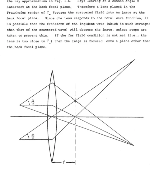
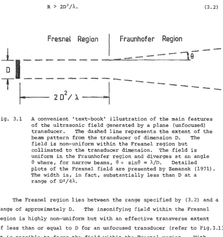
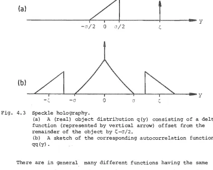
FOR ULTRASO I IMAGI
A thesis
submitted for the degree of
Doctor of Philosophy in Electrical Engineering
from the
University of Canterbury,
Christchurch, New Zealand
by
. s.
~OBINSON
. .(Hons)
ABSTRACT
A new approach to ultrasonic imaging which is designed to form
faithful images in spite of severe propagation distortions is
introduced.
The difficulties associated with the formation of faithful images
of soft mammalian tissue by conventional imaging methods are reviewed.
The degrading effects of transmission speckle are demonstrated
experimentally. The new approach is essentially statistical and
involves the formation and subsequent combination of an ensemble of
images with effectively independent distortions. Experiments show
that the distortions of an ensemble of 128 images formed over
contiguous narrow frequency bands spanning one octave (from 1.7 to
3.4 MHz) are usefully independent and isoplanatic when the propagation
medium is either water on its own or water with animal liver immersed
in it.
It is also demonstrated that, in certain circumstances, a
suit~ble ensemble may be generated entirely within a computer from a
single image. Experimental results for both one-dimensional and
two-dimensional imaging situations show that coherent combination of
such ensembles of images by either speckle interferometry or the
recently developed shift-and-add technique gives worthwhile
improvements. Processing of the images by (modified) Wiener filtering
is also beneficial. An important property of the processing, namely
its ability to reduce the effects of aberrations o~ the imaging
instrument on the processed images, is demonstrated.
The images presented pere are only of isolated objects. The
latter were chosen mainly to allow repeatability of, and unambiguous
interpretation of the results of, the experiments, rather than for
their realism in important practical applications. However, the
success of these preliminary trials suggests that it would be
TABLE OF CONTENTS ABSTRACT ACKNOWLEDGEMENTS PREFACE GLOSSARY CHAPTER CHAPTER l. 1.1 1.2 1.3 1.4 1.5 1.6 1.7 1.8
PART I
CONVENTIONAL IMAGING
A PHYSICAL BASIS FOR ACOUSTICAL IMAGING
Introduction
The Wave Equation for an Inhomogeneous Medium
Inverse and the Wave Equation
,l\pproximate Solutions of the Wave Equation
Rays
Echo-Location
Reconstruction from Projections
Fourier Imaging
1.8.1 Equivalence
1.8.2 Lenses
1. 9 Discussion
2. ULTRASONIC IMAGING PRINCIPLES
2.1 Introduction
2.1.1 Definitions
2.2 Apertures
2.3 Coherent Imaging
2.3.1 Resolution
2.3.2 Focusing
2.3.3 Bandwidth
2.3.4 Processing Sequence
2.4 Incoherent Imaging
2.5 Image Quality
2.5.1 Insonif ica tion
2.5.2 propagation Medium
2.5.3 Speckle
2.6 Discussion
CHAPTER 3. ULTRASONIC IMAGING - PRACTICE
3.1 'Introduction
3.2 Pioneering Work in Acoustical Imaging
3.3 Transduction
3.4 Imaging by Echo-Location
3.4.1 Displays
3.4.2 Scanning
3.4.3 Signal Processing
3.5 Arrays
3.6 Unconventional Im.aging Methods
3.6.1 Holography
3.6.2 Transmission Imaging
3.6.3 Other Methods
3.7 Tissue Characterisation
3.8 Clinical Aspects
3.8.1 Safety
3.8.2 Ultrasound Mammography
3.9 Discussion
PART II
A NEW APPROACH TO ULTRASONIC IMAGING
CHll.PTER 4. SPECKLE PROCESSING TECHNIQUES
4.1 Introduction
4.2 Optical Astronomical Imaging
4.3 Ensemble Formation by Spectral Decomposition
4.4 Speckle Interferometry
57 57 57 60 61 67 70 72 74 78 78 80 84 86 87 88 88 92 95 95 95 98 104
4.4.1 phase Correction 105
4.4.2 Speckle Holography 107
4.4.3 Relation to Stellar Speckle Interferometry 110
4.5 Shift-and-Add
4.6 Stochastic Processing
4.7 Wiener
4.8 Adaptive
4.9 Discussion
CHAPTER 5. THE EXPERIMENTAL IMAGING SYSTEM
5.1 Introduction
5.2 Physical Configuration
5.2.1 Data Sets
5.3 Signal Processing
5.3.1 Measured Waveforms and Spectra
5.4 Coherence
5.4.1 phase Compensation
5.5 Ca1cu1ati0n of Diffraction Patterns
5.5.1 Examples Involving Measured Data
5.6 Image Formation
5.6.1 Processing Options and Examples
5.7 Discussion
CHAPTER 6. EXPERIMENTAL RESULTS FOR ONE-DIMENSIONAL SPECKLE PROCESSING
6.1 Introduction
6.2 Speckle Interferometry
6.3 Shift-and-Add
6.4 Stochastic Processing
6.5 Wiener Filtering
6.6 Discussion
CHAPTER 7. TWO-DIMENSIONAL SPECKLE PROCESSING
7.1 Introduction
7.2 Narrow-Band Imaging
7.3 Wide-band Imaging
7.3.1 Focused Shift-and-Add
7.3.2 Two-Dimensional Shift-and-Add
7.3.3 Transverse Shift-and-Add
127 132 133 135 141 143 145 148 152 155 158 161 161 162 168 179 190 195 199 199 201 205 206 208 214
7.4 Stochastic Processing 217
7.5 Wiener Filtering 221
7.6 Temporal Reconstruction 224
7.7 Computational Requirements 230
7.8 Discussion 231
CHAPTER 8. CONCLUDING REMARKS 235
8.1 Speckle Processing of Ultrasonic Images 235
8.2 Speckle Processing in a Wider Imaging Context 236
8.3 Suggestions for FUrther Research 237
ACKNOWLEDGEMENTS
I am deeply grateful to my supervisor, Professor Richard Bates,
for his guidance, insight and enthusiasm throughout the course of this
research.
Special thaDks are due to Bill Kennedy, Andrew Seagar,
Dr Pet.e!: Gough, Dr Reg Dunlop, Richard Fright and Robert Minard, who
have all assisted in various aspects of this work. I would also like
to thank the staff of the Medical Physics Department, Christchurch
Public Hospital, for conducting very worthwhile courses on biomedical
engineering.
The Electrical Engineering Department has provided a pleasant
working environment for this research. This has been largely due to
the companionship of my colleagues, in particular Dr Graeme McKinnon,
Dr Rick Millane, Dr Pat Heffernan, Dr Jason Bates, Dr phil Bones,
Kathy Garden, Howell Round and Duncan Hall.
During the course of this work I was the grateful recipient of a
Postgraduate Scholarship from the New Zealand University Grants Committee.
Financial support for the project from the Canterbury Medical Research
Foundation is also acknowledged.
My sincere thanks go to M2"s Paula Dowell for willingly undertaking
the task of typing this thesis.
Finally, I wish to thank my paren~s for providing me with the
PREFACE
Ultrasonic imaging is playing an increasingly important role in
medical diagnosis. However, better resolution and lower artefact levels
would further increase the diagnostic usefulness of ultrasonic images.
The recent tremendous improvements in the quality of the images produced
by conventiOfial ultrasonic imaging systems can be largely attributed to
b~tter hardware (e.g. new transducer and display technology). However,
the stage has now been reached where account must be taken of the
distortions of the ultrasonic waves incurred during propagation if
further improvements in image quality are to be realised.
Mammalian soft tissue is a £ar from ideal propagation medium for
ultrasonic waves. Inhomogeneities, of both propagation velocity and
attenuation coef£icient distort the phases and amplitudes, respectively,
of the propagating wavefronts. However, conventional diagnostic imaging
systems assume the propagation medium is homogeneous. Consequently, the
resolution of the images produced by such systems is nowhere near the
theoretical limit. Furthermore, the have a characteristic
'speckly' appearance.
The work reported in this thesis is specifically concerned with new
processing techniques designed to reduce the degradation in image quality
caused by propagation distortions. These techniques are here termed
'speckle processing'. The initial motivation for this work was to assess
whether speckle processing could improve the quality of ultrasonic images
formed through soft mammalian tissue. However, the work has been found
to have significance for any kind of coherent imaging.
The thesis itself is divided into two parts. The first consists
basically of review material which is necessary to place ultrasonic
speckle processing into its proper context. The physical basis for
acoustical imaging is considered in Chapter 1. In ultrasonic imaging,
the incident radiation (i.e. insonification) is under the investigator's
control. Scattered radiation is measured. A description of the
scattering of ultrasonic waves by soft mammalian tissue is embodied in
the wave equation for an inhomogeneous medium. From knowledge o£ the
incident and scattered radiation, it is desired to determine (and
subsequently display) some material property of a body. Conceptually,
scattering. Exact solutions of inverse scattering are only known in
special circumstances and even these may not be useful practically.
Consequently, fram the point of view of 'exact' scattering theory, any
practical ultrasonic image formation process is necessarily approximate.
Various approximate approaches are discussed in Chapter 1.
Chapter 2 deals ~.,ith the principles of conventional ultrasonic
imaging. Factors affecting resolution, such as the aperture size, type
of insonification and propagation medium, are examined and a mathematical
description of the image formation process is developed. The causes and
importance of speckle, which is basically an interference phenomenon, are
also discussed in Chapter 2. Details of practical ultrasonic imaging
methods are re~iewed in Chapter 3. Since the most widely used methods
are based on simple echo-location procedures, particular attention is paid
to such met,hods. However, other ultrasonic imaging methods, such as
holography and computed tomography, are also considered. The potentially
important field of ultrasound mammography is also discussed.
Part II of this thesis is devoted to a new approach to ultrasonic
imaging, called speckle processing, and is mainly concerned with the
author's original work. In Chapter 4, various ultrasonic speckle
processing techniques are described. These were initially inspired by
work done in the related area of high resolution optical astronomical
imaging. However, unlike astronomical imaging, ultrasonic imaging is
(usually) coherent. Also, the propagation distortions of ultrasonic
waves through soft tissue fundamentally differ from propagation
distortions incurred by optical waves in their passage through the Earth's
atmosphere. Therefore, ways of adapting optical speckle processing
techniques to the ultrasonic imaging situation are far from obvious.
An essential preliminary stage of speckle processing involves
obtaining an ensemble of independently distorted images of J:heobject.
The images are then combined in such a way as to preserve the detail of
the true image while reducing artefact levels. Two methods of obtaining
the aforesaid ensemble for ultrasonic speckle processing, namely spectral
decomposition and stochastic processing, are discussed in Chapter 4 along
with various methods of' combining the images.
Carefully controlled experiments were performed to test the efficacy
of the various ultrasonic speckle processing techniques on images of
is described in Chapter 5. This system provides a versatile,
convenient and rather novel means of gathering the required ensembles
of images. In Chapter 6 the results of speckle processing of
one-dimensional images are presented. The images were formed through water
only and also through a combination of water and animal tissue .• :
Noticeable, and in SO"le cases dramatic, improvements were obtained by
speckle processing. The one-dimensional imaging situation was chosen
to demonstrate the properties of speckle processing as clearly as
possible. However, the two-dimensional imaging situation is of far
great.er practical importance. In Chapter 7 the extension of speckle
processing to the two-dimensional imaging situation is described and
experimental results are presented. Again, encouraging results are
obtained. The images are shown to compare favourably with images formed
by a technique closely related to conventional ultrasonic imaging.
This thesis concludes with Chapter 8, which assesses the significance
of the work for ultrasonic imaging and in a general imaging context.
It is emphasised in Chapter 8 that, while encouraging results have been
obtained, this investigation has been of a preliminary nature.
Consequently, further work is needed before these ideas can be applied
..
routinely in practice. Suggestions for further research are 'presented
in Chapter 8.
The work reported in this thesis was performed during the period from
October 1978 until April 1982. During the course of the work the
following papers and presentations have been prepared:
Robinson B.S. and Bates R.H.T. 1980. "The ultrasonic scattering
signature from microcalcifications", Presented at the 20th
Conference on Physical Sciences and Engineering in Medicine and
Biology, Christchurch, New Zealand, August 1980.
Conference proceedings p.26.
Abstract:
Robinson B.S. and Bates R.H.T. 1980. "Wideband ultrasonic diffraction
measurements", Australasian Physical Sciences and Engineering in
Medicine 3, 233-238.
Bates R.H.T. arid Robinson B.S. 1981. "Speckle imaging a new ultrasonic
viewing principle", Presented to the Christchurch Medical Research
Society,Christchurch, New Zealand, November 1980. Abstract:
Bates R.H.T. and Robinson B.S. 1981. "Ultrasonic transmission speckle
imaging", Ultrasonic Imaging 3, 378-394.
Bates R.H.T. and Robinson B.S. 198?. "A stochastical imaging
procedure", To be presented at the Twelfth International Symposium
on Acoustical Imaging, London, July 1982.
Bates R.H.T., Hunt B.R., Robinson B.S., Fright W.R. and Gough P.T. 1982.
"Aspects of speckle interferometric ima.ging", To be presented at
GLOSSARY
The convention that temporal signals and spatial distributions
are denoted by lower case characters and their Fourier transforms are
denoted by the ccrresponding upper case characters is adopted in this
thesis. The following symbols, relations, operators, abbreviations
and functions are not always defined in the immediate context in
which they are used. Note that a dot, i.e. ,.,, is here used to denote
any variable or function.
(i)
t
UJ
x,y,z
u,v
T
A
'IT
j
o ( • )
§
(ii)
«
> (~)
»
E
Symbols
time.
angular frequency.
spatial co-ordinates.
spatial frequency co-ordinates.
a region in space.
wavelength.
infinity.
3.14159 ...
j 2 = -1.
delta function.
section.
vector.
unit vector.
diffraction limited quantity.
Relations
is eq'lal to.
is approximately equal to.
less than (or equal to).
much less than.
greater than (or equal to).
much greater than.
element of.
(iii) Operators
9 convolution.
~ correlation •
• *
complex conjugate.I· I'
magnitude.<.> temporal average.
Re{·}
real part of. / . phase of.L
summation. cos(o} the cosine of.sin ( .) . the sine of.
exp (.) exponentiation (base ~ 2.7l829 ..• ).
in union with.
U
'V gradient Cv =
x
A A
%x + y %y + Z %z}.
dot product.
(iv) Abbreviations
DFT discrete Fourier transform.
D8-0 data set (refer to §5.2.l, Table 5.l).
FFT fast Fourier transform.
Fig. figure.
FM frequency modulation.
po_o processing option (§5.6.l). r.m.s. root mean square.
S&A shift-and-add (§4.5).
TX,RX transducers (Fig. 5.3).
(v) Functions (one-dimensional speckle processing)
m ensemble index (§ 4. 3) .
a(y} incoherent speckle interferometry (§4.4.l).
a (y) coherent speckle interferometry (§4.4.l).
c
c (y) contamination (§4.3). m
e (y) narrow-band stochastic image (§4.6). m
fey) source distribution (§4.3).
ft(Y) temporal reconstruction (§S.3.l).
H (v) ultrasonic transfer function (§4.3).
m
h (y) point spread function (§4.3). m
q(y) scattering strength (§4.3).
q(y) incoherent S&A image (§4.S).
qc(y) coherent S&A image (§4.S).
R (v) distortion function (§4.6).
n
S (v) distorted aperture function (§4.3). m
s (y) speckle image (§4.3). m
sm,n(y) super-distorted image (§4.6).
ss (y) autocorrelation of s (y) (§4.4).
m m
s .. (y) estimate of h (y) (94. 7) .
m m
w (y) narrow-band Wiener filtered image (§4.7). m
w(y) wide-band Wiener filtered image (§4.7).
(vi) Functions (two-dimensional speckle processing)
e (x,y) narrow-band two-dimensional stochastic image (§7.4). m
e(x,y) wide-band two-dimensional stochastic image (§7.4).
(x,y) two-dimensional temporal reconstruction (§7.6).
(x,y) temporal reconstruction (Gerchberg algorithm) (§7.6).
qf(x,y) focused S&A image (§7.3.l).
qc(X,y) two-dimensional S&A image (§7.3.2).
qt(X,y) transverse S&A image (§7.3.3).
s (x,y) speckle image (§7.2). m
1.1 INTRODUCTION
This thesis is concerned with processing methods that have potential
for improving the 'quality' of ultrasonic images of mammalian soft tissue.
The ciim of this chapter is to construct a physical basis for acoustical
imaging. From this basis the fundamental problems inherent in acoustical
imaging become apparent so that the techniques described in subsequent
may be more easily explained.
Soft biological tissue is a far from ideal medium for the propagation
of acoustical energy_ It exhibits spatial variations in den
attenuation and refractive index. In spite of this, pulse echo imaging
systems, based on simple echo-location concepts that make strong
assumptions about the medium, very useful diagnostic information in
practice. From a knowledge of the physics of the situation, and bearing
in mind the increased availability of computers with powerful processing
capabilities, there is cause for optimism that i t may prove possible to
generate even better images than those now routinely obtained with pulse
echo techniques. This perhaps explains the widespread research into
diagnostic imaging that i~ being carried out at present.
The concept of wave motion is fundamental to the treat~ent of
acoustical phenomena. This concept is intuitively satisfying for
(longitudinal) acoustic waves, probably because we are familia.r with
(transverse) waves on water and strings. The propagation of acoustical
waves through biological tissue is governed (to sufficient accuracy for
the purposes of this thesis) by the laws of classical mechanics.
The appropriate form of the wave equation is derived in §1.2. This
serves as the basis for the mathematical model that describes the
scattering of acoustic energy. Solutions of the wave equation are
discussed in §§1.3 and 1.4. The relationship of imaging to the general
problem of inverse scattering is also pointed out. The concepts of rays
and wave fronts are introduced in §l .. 5, where i t is argued that curved
rays usefully describe the propagation of ultrasonic energy in biological
tissue. In §§l. 6 to 1.8 various practical solutions to the inverse scattering problem are dealt with. The approximations and limitations
1.2 THE WAVE EQUATION FOR AN' INHOMOGENEOUS MEDIUM
The wave equation describes the history throughout space and time of
some departure of a medium from equilibrium. The dynamic redistribution
of energy caused by the disturbance is conveniently handled by the concept
of wave motion. This chapter is specifically concerned with the
propagation of acoustic waves in mammalian soft tissue. Because the
physical properties of soft tissue that govern the wave equation exhibit
significant spatial variations it is appropriate to consider the form of
the wave equation for an inhomogeneous medium.
Several assumptions are required to make the analysis tractable. The
medium is assumed to be time invariant, isotropic (i.e. the properties are
independent of the wave direction) and dispersionless with respect to
velocity (i.e. the wave is independent of frequency). It is also
assumed to exhibit adiabatic compression (i.e. negligible heat flow at
ultrasonic frequencies). Furthermore, the shear modulus is assumed
negligible so that only compression waves can propagate and the amplitude
of the disturbance is assumed small enough that the wave motion is linear.
All of these assumptions are physically reasonable and accord w'i th
practical experience (cf. Wells 1977 §§4 and 5). A further assumption
(and one that is often made) that markedly increases the tractability of
the analysis, is that the wave motion is lossless. Unfortunately, this
last assumption is not reasonable from a physical point of view. However,
the attenuation of ultrasonic waves can only be handled in an ad hoc
fashion. Before showing how this is done, it is useful to examine the
various acoustic loss mechanisms.
The loss of acoustic energy by conversion into heat is termed
absorption. Absorption in biological material is frequency, temperature
and amplitude dependent. There are a number of absorption mechanisms
possible. The classical mechanisms for absorption of ultrasound in fluids
are internal friction and heat loss (Malecki 1969 §7). !nternal friction
is caused by viscosity. A shearing force, proportional to the particle
velocity, opposes the motion. The work done in overcoming this force
represents a loss of mechanical energy. Heat loss arises because, in
reali ty, the thermodynamics are described by a politropic process. The
compression is not strictly adiabatic (i.e. it lies on the adiabatic/
isothermal continuum), and there is also thermal radiation. Thus not all
region. Both the classical absorption mechanisms predict that the
absorption depends on the square of the frequency. This relationship
is observed in water, but not in soft biological tissues, where the
frequency dependence is approximately linear. Actually, for soft tissue
at typical diagnostic frequencies, the dependence lies somewhere between
fl.a and fl.2 (Pauly and Schwan 1971) . Wells (1977 §4.5) states that the
value of absorption predicted by the classical viscosity mechanism is
about two orders of magnitude lower than that observed in practice. In
view of these discrepancies, classical absorption is generally discounted
as the predominant absorption mechanism in soft tissue.
Relaxation phenomena occurring at the macromolecular level
(cf. Malecki 1969 §7.4) can explain the observed linear frequency
dependence. Molecular relaxation refers to a process whereby energy is
shared between various 'compartments' (e.g. translational and rotational
kinetic energy of the molecule). When the energy of one compartment is
altered externally, the sharing process takes a finite time to achieve
equilibrium. If the period of vibration is of the order of this
'relaxation' time, not all of the energy can be recovered from the
original compartment and loss results. For frequencies either much
greater or much less than the relaxation frequency, there is either no
energy transfer between compartments, or complete equilibrium is reached.
Thus the absorption is at a maximum around the relaxation frequency.
Several relaxation processes at staggered relaxation frequencies can
explain the observed linear frequency dependence of absorption in
biological tissue (Pauly and Schwan 1971, Edmonds 1962).
Unlike the classical mechanisms, molecular relaxation also
successfully accounts for the observed linear relationship between
velocity dispersion and absorption (cf. Wells 1977 §4.5). It should be
noted that the magnitude of the dispersion (less than 1% per frequency
decade) is small enough that it is usually neglected. However, any
acceptable absorption theory must be able to explain it.
Another approach is to use a visco-elastic model. The Voigt model
(Raichel 1972), which places the viscous and elastic components in
parallel, describes the behaviour of viscous liquids which manifest some
degree of solid-like behaviour. Thus it seems a physically reasonable
basis for a model of mammalian soft tissue. Ahuja (1979) claims
frequency with observed frequency dependence of soft tissue.
Knowledge of the exact mechanisms of ultrasonic absorption in soft
tissues is, at this stage, still very tentative. One of the main problems
is the paucity of data for modelling. For this reason, it does not seem
worthwhile to attempt to include absorption, as a function of fundamental
tissue properties, into the wave equation. However, absorption is always
manifested as a phase difference between the instantaneous pressure and
particle displacement about some point (Skudrzyk 1971 §§2 and 13).
Therefore, no matter what the mechanism, absorption can be incorporated into
the wave equation by introducing a complex, frequency dependent value for
the acoustic velocity. This point is further discussed after the
space-frequency form of the wave equation (equation 1.7) is derived.
The wave equation for a lossless medium is derived by considering the
physics of a small element of the medium disturbed by the propagating wave
(Skudrzyk 1971 §13). This yields two useful approximate equations. The
first is Euler's equation for irrotational flow which is an expression of
Newton's Second Law of motion:
dV/dt
=
-'iJp/p (1.1)The second is the 'equation of continuity' for the medium which is a
combination of the law of conservation of mass and the state equation:
(1.2)
where V is velocity of the infinitismal volume element (Le. the particle
velocity in a solid), P is the pressure, p is the equilibrium density of
the medium, and c is the velocity of the acoustic wave.
of position in an inhomogeneous medium.
The above is an Eulerian description of motion.
c is a function
The co-ordinate
system for the fluid properties is fixed in space and the pressure,
velocity etc. refer to whichever particles happen to be at a 'point' at a
given time. An alternative bu~ for this purpose, less convenient
approach describes the properties of an 'identified' particle. Thus, in
the Lagrangian description, the co-ordinate system moves with the particle.
The velocity V may be .eliminated by differentiating Euler's equation
with respect to space and the equation of continuity with respect to time,
a/at
('V.V) - 'V. ('VP /p),
(1. 3)and
(1. 4)
combining equations (1.3) and (1.4) yields the pressure wave
equation for an inhomogeneous medium.
('V%) .\jp (1. 5)
Both V and p may be obtained from P so that only the wave equation in P
is necessary to obtain all the acoustic variables.
The space-frequency dependence of P characterises it as completely
as does its space-time behaviour.
and temporal components, i.e.
Writing P in terms of its spatial
P (x, t) P (x) exp (jwt) (1. 6)
the space-frequency wave equation is obtained from (1.5) by taking its
temporal Fourier transform. Thus
+ (wlc) (Vp/P) ·'VP (1. 7)
where the exp(jwt} factor, common to each term, has been dropped (but
it must be understood) . The spectral decomposition implicit in (1.7)
allows absorption to be handled much more readily than for the
spatio-temporal form of the wave equation (1.5). Absorption is accounted for
phenomenologically by making c a complex quantity. Its imaginary
part, which is frequency dependent for soft tissue, determines the
amount of absorption. However (1.7) treats each spectral component
of the wave separately so that dispersion is not a difficulty. Since
linear wave motion is assumed, the separate spectral components may be
combined to give the total solution.
It is convenient to define the (complex) acoustic refractive index
n of the medium relative to water as
n c /c
where c is the acoustic velocity in water.
w The wave number in water is
k
=
wlc wand the term (wid 2 in (1. 7) is then k2n2.
(1. 9)
The standard form of the wave equation is obtained from (1.7) by
defining a wave function ~ such that
p
=
( 1.10)Substituting (1.10) into (1.7) gives
(1.11)
where
(1.12)
It is apparent from (1.12) that II may be neglected with respect to
k2n2 when the spatial variation of density is sufficiently small (i.e. the ,
medium is almost homogeneous) • This is known as the Picht-Bruns
approximation and basically says that variations in the wave velocity of the
medium predominate over density variations in causing scattering. For the
case of ultrasonic wave propagation through soft biological tissue, this
approximation is not really valid (Chivers 1978) and so it is not used here.
1.3 INVERSE SC~TTERING AND THE WAVE EQUATION
A physical interpretation of the wave equation may be gained by
re-arranging (1.11) to give
-ql/J (1.13)
where
q == tll + k 2 (n· -2 I) (1.14)
(1.13) has the form of the wave equation for a homogeneous medium in which
radiating sources are imbedded. Note that no terms relating to spatially
varying properties of the medium are present on the left hand side of (1.13).
The term on the right hand side of (1.13) represents the apparent density of
the aforesaid radiating sources. These are not true sources since they are
dependent on l/J. They are therefore called 'volume' or 'polarisation' sources
(cf. Bates and Ng 1972). Such sources are entirely due to scattering (and
the medium and can (rigorously) be regarded as the 'seat' of the
sca ttered field. For a homogeneous medium, both terms on the right
hand side of (1.14) are zero and so the right hand side of (1.13) is
also zero. Therefore, for the case of a homogeneous medium, there
is no scattered field and an incident wave propagates unperturbed
according to the ~omogeneous wave equation.
A solution of the wave equation is obtained in the following manner.
The total wave function ~ is divided into the sum of the incident and
scattered wave functions, i.e.,
~
=
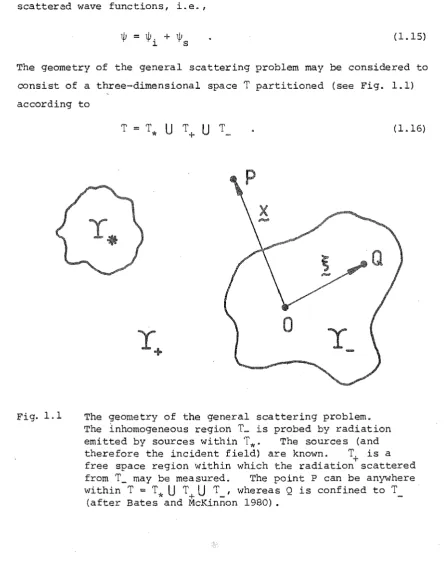
~. ~ + ~ s (1.15)The geometry of the general scattering problem may be considered to
consist of a three-dimensional space
T
partitioned (see Fig. 1.1)according to
Fig. 1.1
( 1.16)
The geometry of the general scattering problem. The inhomogeneous region T_ is probed by radiation emitted by sources within
T*.
The sources (and therefore the incident field) are known. T+ is a free space region within which the radiation scattered from may be measured. The point P can be anywhere within T=
T*U
TU
T , whereas Q is confined to T+
[image:21.595.57.504.237.806.2]T
is a homogeneous medium (e.g. water with n=
1) that surrounds two isolated +regions,
T
andT .
*
-
T*
has imbedded in i t known sources that give rise tothe field ~. that is incident upon the region
T_.
1. T is the inhomogeneous
region (or 'scattering object') that gives rise to the scattered field ~ . s An arbitrary point in
T,
with position vector x, is denoted by P and anarbitrary point restricted to T_, with position vector ~, is denoted by Q.
Now, consider the wave equation describing an arbitrary wave function
1). propaga ting through free space, i. e •
=:: -5 (1.17)
where 5 is the density of the sources that give rise to ¢.
The solution of the differential equation (1.17) is (Jones 1964 §l),
exp(-jklx - ~I)'
5(~,k)
4'TfIX
=
~I
dv, (1.18)where dv is the element of volume (i.e. dv
=
d3~),
and j =;.:r .
Nowpostulate that all space is free, with the inhomogeneities within
T
being replaced by apparent source densities (cf. equation 1.13). Sincethe sources of the incident field lie entirely within
T*,
i t follows that( 1.19)
Combining (1.13) to (1.15) and (1.19) gives
-q~ P E T , (1.20)
where q
=
0 outside T .and (1.18) to be
The integral form of (1.20) is seen from (1.17)
exp ( - j k
I
x - ~I )
~(~,k) 4'Tf1~
=
~I
dv . (1. 21)There are two general classes of scattering problem. The direct
problem involves determining the scattered field, ~ , given ~. and q.
s J.
Difficulties in the direct problem lie mainly in the degree of accuracy
required in the solution (cf. Keller 1957, Harrington 1968).
class of scattering problem is known as the inverse problem.
determining the material properties characterised by q, given
The second
This involves
~. and ~ .
Thus the inverse problem is synonomous with the gen~ral imaging problem
(in which knowledge is gained about a body from the manner in which it
scatters incident radiation), In contrast with the direct problem,
the inverse problem still poses conceptual uncertainties, Exact
solutions exist for a few special cases (cf, Newton 1974, Bates 1975),
However, even in these cases, practical computational difficulties
normally allow only an approximate solution to be calculated
(cf, McKinnon 1980),
In the usual imaging situation, the imaging instrument is rem':lt.e
from the body, This means in practice that ~ can only be measured s
in
T+,
T+
U
T",.in (1. 21)
Therefore the total wavefunction ~ is also only known in
This leads to a difficulty, since the integration of ~
is throughout the volume of the scattering region
T
Itis apparent from (1.13) and (1.17) that the equivalent source density
within
T
consists of the product of what it is wished to characterise(i.e. q, the material properties) and the total wave function. Both
of these unknown terms are present under the integral sign of (1.21).
Therefore, there is a dimensionality problem (cf. Bates and McKinnon
1980) • Since ~ is entirely radiating away from
T ,
it is completely sdescribed by a measurement on a single closed surface in T+ surrounding
T.
Remembering that the wave function is a function of space andfrequency (i.e, k), the measured data is clearly three-dimensional
(the two dimensions of the surface and one of frequency). However,
the unknown quantity is four-dimensional (three dimensions of the
volume of
T
and one of frequency). Consequently an exact solutionof the inverse problem involves continuing ~ analytically throughout
T.
Any method attempting to do this will obviously be sensitive toerrors that inevitably exist in the measured data (cf. Deschamps and
Cabayan 1972).
1.4 APPROXIMATE SOLUTIONS OF THE WAVE EQUATION
Since an exact solution of the inverse scattering problem as posed
\
in §1.3 is usually impractical, it is common to make an approximation to
(1. 21) . The simplest approach is known as the Born (or alternatively,
in classical field theory, the Rayleigh-Gans) approximation. It is
assumed that the region T_ is sufficiently tenuous (i.e. similar to T )
- +
that the total wave function in (1.21) may be replaced by the (known)
1./1 (x,k) s ~
exp(-jkl:
q(~,k) 1./Ii(~,k) 4~1:
_
(1. 22)The condition for the Born approximation to be valid is that the
scattering is very weak, i.e.
(1. 23)
(1.23) means in effect that radiation scattered more than once is
negligible. In addition, the phase of the wave propagating through T
must undergo negligible change due to the variable refractive index over
all T • This condition is given by
(1. 24)
where L is the largest linear dimension of T • Relation (1.24) shows
that the validity of the Born approximation depends on both the deviation
of the refractive index from unity, and the extent of the region over
which the deviation occurs. For example, given only a 1% deviation in
velocity, (Le. n 1.01) the approximation breaks down (i.e. the phase
is in error by, say, ~/2) after 25 wavelengths. In soft biological tissue
at a typical diagnostic frequency of 2MHz, this corresponds to a distance
of less than 20 rom. The Born approximation is most suited to regions in
which weak scatterers, whose dimensions are limited to no more than a few
wavelengths, are imbedded in a medium of constant refractive index.
The Rytov approximation avoids some of the imperfections of the Born
approximation. The method is similar to that of the Born approximation
except that the wave equation is first transformed into a Riccati equation
which (as in the Born approximation) is solved to the first order (cf.
Wade et al. 1979). The advantage of the Rytov approximation is that it
only requires the integrated deviation of the refractive index from unity
per wavelength to be small (Chernov 1960 §5). Therefore the size of the
scattering domain is unimportant. The Rytov approximation describes the
wave function within T more accurately than the Born approximation for
large scale inhomogeneities (i.e. when 'forward scattering' predominates
this is discussed more fully in §1.5). However, it still does not
the correct phase for the scattered wave function.
Bates et ale (1976) have developed an extension to the Rytov
approximation. Based on the W.K.B. solution of the wave equation (cf.
§1.5, equation 1.31), it takes account of the term neglected
Since the additional term allows for extra phase shifts (and also,
partially, refraction) caused by variations in refractive index, the
extended Rytov approximation estimates the phase of the scattered
field more accurately than either the Born or conventional Rytov
approximations. This has been verified numerically by Dunlop
et aZ.
(1976) .
The essential point is that both the Rytov and extended Rytov
approximations can be written as equations of the same form as (1.22),
and so can be solved for the appropriate scattering function q in the
same manner. A simple inversion procedure is discussed in §1.8. For
the extended Rytov approximation, q is defined differently than in
(1.22). In this case the various terms of q may be separated out by
obtaining solutions at three different frequencies (i.e. three sets of
measurements for different k). In principle, of the three
approximations, an imaging method based on the extended Rytov
approximation should result in the most faithful images. Kaveh
et
aLe(1974) investigate imaging methods based on approximate solutions of
the wave equation. They term their approach 'diffraction tomography'
(see §1.7) and use both the Born and conventional Rytov approximations.
1.5 RAYS
The concept that wave motion can be described in terms of the
propagation of rays is very useful. Ray descriptions greatly ease the
analysis of certain problems (i.e. those where the required assumptions
are applicable). Rays represent a high frequency approximation. The
wavelength should be smaller than the scale of the inhomogeneities of
refractive index so that local propagation may be considered as a plane
wave. Rays form the basis of Geometrical Optics, which is successful
in solving many optical problems not including diffraction.
It is useful to separate the total wave fUnction into an onward
propagating part ~, and a deflected part ~d'
(1. 25)
~ is similar to ~. but includes any significant 'forward; scattering
~
(and also specular reflections) from large scale inhomogeneities. ~
approximation. In typical echo-location procedures (refer to §§1.6 and
3.4) a beam is used to probe a region. ~ is the transmitted beam which
may be regarded as a 'bundle of rays'. ~d represents that part of ~
that is scattered out of the path of the beam. ~d arises from scattering
by small scale inhomogeneities and is assumed small everywhere compared
with ~.
The following analysis is known as the W.K.B. or phase integral method.
Alternative approaches are used by Mawardi (1970) and Korpel (1970). A
useful. approximate representation of ~ is the asymptotic series (Eorn and
Wolf 1970 §3.1)
00
~
=
exp(-jks)L
m=Ok-m A
m (1.26)
which has the form of a tube of rays. ks(x) is the phase of the wave
function. Therefore surfaces where s(x) == constant are wavefronts, and the
ray propagates in the direction of Vs. Substituting this expression for
~ into the wave equation (1.11) gives a series in inverse powers 0f k.
Terms associated with a particular power of k can be treated separately.
2
From the term in the highest power (i.e. for k ), by equating the
coefficient to zero the eikonal equation is derived, i.e.
The solution of (1.27) is
2
= n
x ~
s ==
Ix
n d,Q,~O
(1. 27)
(1. 28)
where d~ is the element of arc along the path of the ray from the starting
point ~O to the point x. s may be thought of as the 'acoustic path length'.
The ray takes the path in space such that s is either minimised or unchanged
(i.e. stationary) compared with nearby paths. Thus the eikonal equation
incorporates Fermat's principle from which the Geometrical Optics laws of
reflection and refraction are readily derived.
In a similar fashion, considering the coefficients of terms in k1 gives
the first transport equation,
(1. 29)
Vs = ~n (~ is a unit vector in the direction of the ray) to give
A o = -!
n (1.30)
Rays represent a high frequency approximation. For sufficiently
high frequencies (i.e. k is large) the series of (1.26) can be
approximated by the first term. Therefore, the appropriate form for
a plane wave· (as for example, is found far from a localised source)
propagating in a tenuous inhomogeneous medium is
~ 1
~ = (E/n~) exp(-jks) (1.31)
where E is the radiation pattern of the source, (i.e. E varies across
the bundle of rays). The n-! term accounts for amplitude changes
as the velocity of the ray changes. Absorption is allowed for
because n, and hence s, may be complex. The wave function of (1.31)
is usually a valid description of the propagation of ultrasonic waves
in biological soft tissue. Physically, it means that the acoustic
energy can be thought of as travelling as rays. However, the rays in
general follow curved paths due to variations in the refractive index.
In other words, a plane wave entering biological tissue from water
undergoes phase distortion so that, although generally propagating in
the forward direction, the wave fronts are no longer plane.
It should be emphasised that the rays of Geometrical Optics do not
allow for diffraction phenomena. However, in situations where
diffraction is important, it can be handled in a ray-optical manner by
an extension of Geometrical Optics called the 'geometrical theory of
diffraction (G.T.D.)' (Keller 1962, James 1976). In this method, rays
are still used to describe the propagation. Usually, most of the
scattered field consists of reflected or refracted rays described
by conventional Geometrical Optics. However, when discontinuities
(i.e. inhomogeneities whose radii of curvature are less than a
wave-length) are encountered, 'diffracted' rays are generated. Such
discontinuities may be small spheres, edges, corners, vertices etc.
Exact solutions for the diffracted rays may be calculated for each
of these simple discontinuities. The total field then comprises the
contributions from Geometrical Optics rays and the diffracted rays.
The temporal wave function is easily derived from (1.31)
include the temporal spectrum as well as the source radiation pattern, i.e.
E
=
E (x ,W) • Then, by including the exp(jwt) time dependence (understood from (1.7) onwards), and remembering that k = w/c , the following Fourierw
transform relation is obtained:
00
f
(E(::,W)I9-
n!) _0000
=
r
(E(::,W)19-
n!)J
- 0 0
exp(-jks) exp(jwt) dW
exp [ j w (t - sic ) 1 dw
w
'¥(x,t - sic) I 9- n! (1.32)
w
'¥(t) is called the waveform of the signal. The wave function '¥(x,t) is a
particularly useful description for wideband signals, such as pulses,
propagating in spatially confined wave bundles (beams). This type of wave
function is commonly used in simple pulse echo imaging systems. Energy
conservation considerations necessitate the introduction of the 1/9- amplitude factor into (1.32) to account for beam spreading due to diffraction.
1.6 ECHO-LOCATION
The most widely used imaging techniques employing ultrasonic waves are
based on the principles of echo-location. The region
T
(Fig.l.2) I isassumed to contain small weakly reflecting bodies imbedded in an otherwise
homogeneous medium (with n
=
1 everywhere). Since n=
1 the ray paths arestraight and the acoustic path length s (from equation 1.28) is simply the
physical length
1:1.
With reference to Fig. 1.2, a transducer that canboth transmit and receive is located at the origin 0 and emits a narrow
r.
beam in the direction defined by
r.
Letting1:1
=
r,
and denoting thetransmitted waveform by '¥, i t follows from equation (1.32) that
'¥(r,t)
=
(l/r) '¥(t - ric)w (1. 33)
If A(r) is the reflectivity of the small scatterers in
T ,
then thedeflected part of the wave function (i.e. echoes) received back at the
origin is given by
'¥ (t - 2r/c ).
w (1. 34)
simply obtained by equating the time delay of the received waveform
to range. The resolution in range is determined by the temporal
resolution. A complete three-dimensional image of the reflectance
function may be formed by scanning the transducer about 0' (i. e.
'"
changing the direction of r) so that all of T is probed.
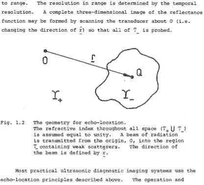
Fig. 1.2 The geometry for echo-location.
The refractive index throughout all space (T+
U
T_)is assumed equal to unity. A beam of radiation is transmitted from the origin, 0, into the region T_containing weak scattxrers. The direction of the beam is defined by r.
Most practical ultrasonic diagnostic imaging systems use the
echo-location principles described above. The operation and
terminology of such systems is the subject of Chapter 3. However, aspects are briefly reviewed here in order to relate pulse echo
imaging to the inverse scat,tering problem.
A wide band signal in the form of a narrow pulse is transmitted.
This gives good temporal resolution and also allows extremely simple
signal processing since the location of the scatterer is determined
by a time/range 'gate'. The narrowness of the beam is determined
by 'the dimensions (i.e. aperture) of the transducer, and the
distance
1:1.
Attenuation is usually allowed for in an approximatemanner (cf. Maginness 1979) by assuming an arbitrary value. The
total weakening of the ray as it propagates is due to spreading
(Le. diffraction) and attenuation. The latter comprises
scattering from small inhomogeneities and pure absorption (i.e.
conversion of acoustic energy to heat) . The attenuation coefficient
of mammalian soft tissues (e.g. liver, muscle, etc.) is of the order
[image:29.595.80.498.99.479.2]probably the most significant part. Scattering within a particular tissue
type is generally weak although stronger sca·ttering occurs at tissue
interfaces.
It must be emphasised that the faithfulness of the image formed on the
basis of elementary echo-location ideas depends on how closely the medium
conforms to the simple model used to derive (1.34). In practice, geometrical
distortions occur because the ray paths in soft tissue are curved and the ray
does not travel at constant velocity. Both types of distortion caus~ the
image of a point to be shifted (or 'misregistered') with respect to its true
position. The scattering strength determined for each image point may also
be in error, since the precise attenuation of the ray is unknown. This
causes • shadowing' and 'enhancement' effects in the image. It is interesting to note that many of the errors and anomalies (provided that they are
recognised as such) that occur in clinical images, in fact, convey valuable
diagnostic information to the trained observer (cf. Kobayashi 1977,
Nicholas 1980).
The model used for echo-location is very similar to that of the Born
approximation, i.e. weak scattering and negligible variation in n is
assumed. Biological soft tissue generally satisfies the first condition
but not the second. Also, as explained in §3.4, practical diagnostic echo~
location systems (cf. Wells 1977 §5) use small numerical apertures and
neglect the phase of ~d (i.e. incoherent signal detection of the pulse is
used) . Therefore, in the context of inverse scattering theory,
echo-location procedures represent only very approximate inversions of (1.22).
1.7 RECONSTRUCTION FROM PROJECTIONS
If the rays propagating through a medium are known to travel in straight
lines, then an exact solution to the inverse scattering problem may be gained
by employing projection (or Radon transform) theory (cf. Bates and Peters
1971) • An image of some material property,
a
say, of the medium isreconstructed from measurements of the projections of 0(X). A projection
essentially consists of integrals of 0(x) along straight lines.
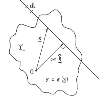
"-dimensions the projection f(a~) is defined by (refer to Fig. 1.3)
f(a~)
AJ
cr(~)
dl,;'x=a
In two
where ~ • x
=
a defines the line of integration. d,Q, is thedifferential element along this line (which is perpendicular to the
'"
unit vector ~ , and a distance a from the origin).
Fig. 1.3 The geometry for c~mputed tomography.
The projection f{a;) is,,,the integral of
a
along the line perpendicular-to a~Each projection is a function of angle (i. e. of ~) and position
(a) . A complete set of projections is obtained by varying the angle
over TI radians. Making use of delta function notation, (1.35) can
be rewritten as
ff
a(x) <5{a - ~. x) dx ' f (1. 36) where the integration is over the entire plane. Taking theone-dimensional Fourier transform of (1.36) (at the angle defined by
~) with respect to a gives
r (S~)
=Iff
a(x) <5 (a ~ 'x) expel dxda-
~H
a(x) exp(j2TIB ~ ·x) dx-
-(1. 37)
[image:31.595.118.461.160.485.2]
"-Defining a~
=
u, then~
F(u) ==
If
a(x) exp (j21T u.x) dx ~ (1. 39) which is simply the two-dimensional Fourier transform of a(x). Thus thespatial distribution of
a
may be obtained simply by computing one-dimensional Fourier transforms of each one of the complete set of
"-projections, laying these at the appropriate angles (given by ~) in Fourier
space, and then calculating a single two-dimensional inverse Fourier
transform. Practical implementation of image reconstruction from
projections is usually by the 'modified back projection' algorithm (cf.
Brooks and Di Chiro 1976). This involves convolving the projections with
a 'filter function', spreading (or 'back projecting') the modified
projections back along the appropriate ray paths and accumulating the values
of each modified projection at image points intersected by each ray.
Modified back projection is equivalent to, but in practice, computationally
more efficient and accurate (since interpolations are performed in the
image as opposed to the Fourier domain) than the method suggested by (1.39).
The whole procedure is generally termed 'computed tomography',
For ultrasonic computed tomography
a
has been variously taken as attenuation coefficient (Greenleafet aZ.
1974), refractive index(Greenleaf
et
al.
1975, Bates and Dunlop 1977), integrated attenuation coefficient (Dines and Kak 1979), and reflectivity (Norton and Linzer 1979) .There is presently a great deal of research into ultrasonic computed
tomography. However, image quality is not as impressive as that obtained
in x-ray computed tomography. This is, for example, evidenced by
comparison of the images presented by Kak (1979) in a review of diagnostic
imaging methods based on computed tomography.
Ray curvature appears to be a significant factor in the degradation of
images obtained by ultrasound computed tomography. The integration in
(1.35) should be along the true ray path (i.e. of the form of equation 1.28).
Procedures have been suggested by Johnson
et aZ.
(1975a), Schomberg (1978), and Bates and McKinnon (1979) to correct for ray curvature. Essentiallythe methods involve reconstructing the refractive index assuming straight
ray propagation, and then, from the initial estimate of refractive index
(and hence ray paths), applying an iterative correction. An approach
similar in concept to this has also been suggested by Vezzetti and Aks (1979)
Born approximation as an initial estimate .. No convergence bounds
have been found for the above methods and it is uncertain whether
the procedures necessarily converge to the correct value for n. In
fact, McKinnon and Bates (1980) point out that there can exist
'forbidden regions' into which (minimum propagation time) rays never
penetrate. It is, therefore, impossible to faithfully reconstruct
a within these regions.
A different approach towards allowing for ray curvature is to
treat computed tomography as a problem of inverting the wave equation
(cf. Mueller
et aZ.
1979, Kavehet aZ.
1979, Muelleret aZ.
1980). Making use of the Born or Rytov approximations, the solution of thewave equation can be in terms of computed tomography with
refraction (at least partially) accounted for.
A significant advantage of ultrasonic computed
tomography is that, in principle, quantitative images may be formed.
At every point in the image a value of some acoustic parameter (e.g.
acoustic velocity or attenuation coefficient) is calculated. Provided
that the image values are accurate, various tiss~e types represented
in the image may be differentiated rapidly and objectively on the
basis of these values. For example, normal, benign and malignant
breast tissue exhibit significant differences in attenuation
coefficient (Calderon
et aZ.
1976).Echo-location procedures normally yield only qualitative images.
The reasons for this are outlined in the previous section. Tissue
characterisation from such images is therefore very subjective since
it is based on how the image of some region of tissue 'appears' to
the observer.
1.8 FOURIER IMAGING
When the Born approximation holds, (1.22) can be inverted to solve
for the scattering function q by simple Fourier methods (Wolf 1969).
A similar procedure is used in the case of the Rytov and extended
Rytovapproximations (Iwata and Nagata 1975, Bates
et aZ.
1976). The incident field is made a plane wave, defined byl~ . (x ,k)
where the vector wave number k defines the direction ~s well as the
frequency of the plane wave.
large distance from
T
(seeThe scattered field, lPs~' is measured at a
1.1), Le.
1:1
»
(1. 41)so that the term I~-
§I
in (1.22) can be approximated by considering only the first two terms of the binomial expansion, which results i.n(1. 42)
Where I::-~I appears as the amplitude factor in (1.22) it can usually be
replaced simply by the first term of (1.42), i.e.
I
~I.
However, this cannot be done where1::-
~I appears in the complex exponent. It is usual to consider the case where the smallest term of (1.42) can be neglected.This is possible when its contribution to the total phase is small (the
normal limit is
n/2
radians). Therefore, remembering that ~ is bounded by the condition is(1. 43)
where k (1.43) may be rearranged to give
2
1:1
> 21~1II..
(1.44)This is the familiar far-field or Fraunhofer condition. It means that the
scattered field is measured so far from T_ that
lp
takes the form of planes
waves propagating radially outwards from
Using (1.40) to (1.44), (1.22) can be rewritten as
k2 exp(-jkl:::l)
4n
:1
Iff
T
kx
q(~,k) expr-j[~ - ~'I]'
I:
dv.
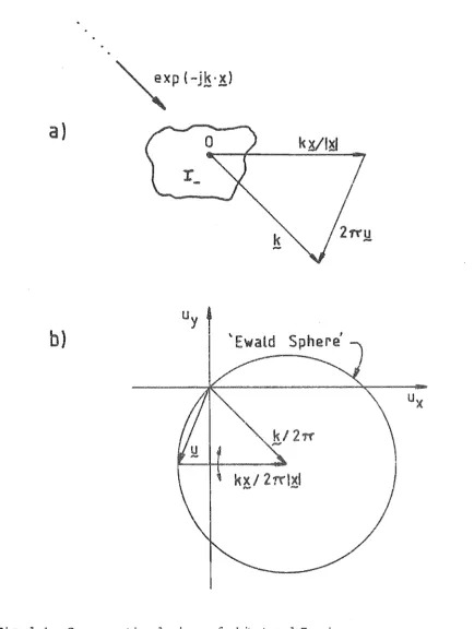
(1.45)Provided that ~ is measured at a constant radius from the origin (i.e. s
I~I = constant) and the vector u is defined by (see Fig. 1.4a)
k kx/lx
1
(1. 46)(1.45) becomes
Q (u)
f
(
\ (I q(~) exp(-j21TU'~) dv J jJ
(1.47)
T
where Q(u) incorporates both 1j; and the constant
Since the right hand side of (1.47) is a Fourier integral, it is
evident that q(~) can be recovered from the scattered field simply
by taking an inverse Fourier transform. However, to specify
Q(u) completely, more than one measurement of ~ is required s
(remember u is a function of both k and x) . For a given incident
wave, ~s is measured over a spherical surface
(1:1
=
constant). From Fig.l.4b it is seen that the spatial frequency variable, u,also traces out a spherical surface, (which is known as an 'Ewald
sphere', cf. Guinier 1963 §l) in Fourier space as x varies. The
surface of the Ewald sphere grazes the origin and from (1.46) its
diameter is 2/A. Thus the spatial frequency components of Q
available from the measurement of ~ , are restricted to
s
2/'A (1. 48)
It is shown in §2.3.1 that spatial resolution is proportional
to the reciprocal of the spatial frequency bandwidth. Inspection
of (1.48) leads to the conclusion (which is very reasonable from a
physical point of view) that the resolution of the imaging system
is fundamentally limited by, and of the order of, the wavelength.
To obtain all the (spatial frequency) spectral information on
the surface of the Ewald sphere requires that the measurement of
¢
be made on a spherical surface enclosingT .
s - Frequently, for
practical reasons, measurements cannot be made over the entire
spherical surface. The physical aperture of the imaging instrument
is that part of the enclosing surface over which
¢
is measured. sWhen the aperture does not extend over the entire surface, resolution
is degraded because the spatial frequency bandwidth is reduced.
The resolution theoretically possible from given aperture dimensions
is known as the 'diffraction limit'. Apertures are further
discussed in §2.2.
1.8.1 Space-Frequency Equivalence
The spatial frequency components available from a single
measurement of ~ are restricted to those corresponding to values
s
of u lying on the surface of the Ewald sphere. Thus a single
measurement gives only two-dimensional information. In order to
three-a)
b}
Fig. 1.4
\ Ewald
Cross-sectional views of object and Fourier space.
(a) Object space. ~ is defined by the vector difference between the incident and scattered waves.
(b) Four ier space. As x rotates, u traces .out the surface of the E1tlald sphere.