A new transfer function analyser

University of Warwick institutional repository: http://go.warwick.ac.uk/wrap

A Thesis Submitted for the Degree of PhD at the University of Warwick

http://go.warwick.ac.uk/wrap/73949

This thesis is made available online and is protected by original copyright. Please scroll down to view the document itself.

A NEW

TRANSFER FUNC'l'ION ... NALYSER

by

James R. Robertson.

h thesis submitted to the University of Warwick for the degree of

Doctor of Philosophy.

School of Engineering Science

ABSTRACT

This thesis investigates the concept and design of a portable on.line transfer function analyser (TFA). It is eminently suitable for the identification of plants and other

controlled feedback systems in which normal operating records are available.

A point by point representation in the frequency domain, requiring a maximum of three records, allows Nyquist plots to be carried out, either visually or by plotter facilities. The basic theory relies heavily upon statistical concepts whereby, least squares estimates of the transfer function are obtained from

a combination of heterodyning, exact filtering and adaptive loops. The resultant output, on both channels (real and imaginary), is the culmination of the solution to two linear differential equations with stochastic coefficients, so mechanised when the adaptive loops reach a stable equilibrium.

Throughout, emphasis is placed upon the electronics combining the best of analog and digital techniques, in order that six

parallel paths may be analysed in similar mode. This is especially

true of the heterodyning and filtering operations. Practical shortcomings of the instrum~nt ar~ noted by comparing estimates with those from the best currently available commercial apparatus, operating on deterministic signals. ~xamples of a feedback loopt subjected to both deterministic and random stimulii, with and without the pre~ence of extraneous noise sources, are used to illustrate the ease and simplicity by which the instrument can

be used in place of complex computing schemes, which tend, in consequence, to be solely of local academic interest.

of four papers to the technical press. Two of them deal,

exclusively, with a capacitor ratio commutated filter - not apparently described in publications to date - which is also

the subject of a proposed patent application in conjunction

.1.CKNO'rlLEDGEMENTS

This thesis represents work carried out at the University of Warwick, by the author, during the period October 1968 to

December

1970.

It was sol~ly conducted by him, except where due acknowledgem~nt has been made to referenc~s.

During this period, he was financed by the Science Research Council to develop a new method of transfer function analysis and is, accordingly, gruatly indebted fvr their assistance.

He expresses his thanks to the School of Engineering Science for the experimental equipment available and to his sup&rvisur, Dr. M. T. G. Hughes, for his initiation and helpful discussions of th<:: project.

Finally, he appreciates the competence of his Senior Technician, Mr. M. P. Bell, whose interest in printed circuit boards allowed a compact instrument to be built.

Abstract.

Acknowledgements. Contents.

CONTENTS

Glossary of Principal Symbols.

CHAPl'ER 1 Introduction.

1.1 Review of Continuous Frequency

~stimation using Computational

1.2 Review of Continuous Frequency

1 HespGDse Hethods. 2

Response Estimation using Special Purpose Hardware. 4 1.3

1.4

CHAP'rEH 2

2.1

2.2

2.2.1

2.2.2

Motivation of Thesis. Contribution of Thesis.

Theoretical Study of a New Transfer Function Analyser.

Introduction.

Basic Concepts.

Bias Aspects of Cross-Spectral

Identification.

Variance Aspects of Cross-Spectral Identification.

An Adaptive Modelling Technique. Parameter Adjustment.

2.4 Statistics of an Adaptive Loop Transfer Function Analyser.

2.4.1 An Approximation to the Mean Solution

of the Model Gains.

An Approximate Discussion of Bias.

An Approximate Discussion of

Convergence. Figures(2.1)-(2.4).

CHAPTER 3 Novel Electronic Filtering Technique~. Introduction.

Aspects of the Resolver. Theory of the Resolver. Practical Considerations. Minimisation of Harmonics. Operation of the Resolver.

3.7 Factors Affecting the Aoouracy of the Resolver.

Harmonic Breakthrough. Aspects of Filtering. oampled Data Filters. Commutated Filters.

3.10 The Capacitor-Hatio Commutated

CHAPTER

4

4.1 4.2 4.2.1

Filter (CRCF).

Construotion of a CRCF. Figures (3.1) - (3.13).

Complete Instrument Orgaui.~tic)ll. Introduction.

Frequency Sweeping. Digital Techniques.

Heri ts of Digital Techniques. Hybrid Techniques.

Automatic Incremental Sweep. Design of the Incremental Sweep Counter.

Rate of Change of Incremental Sweep. Summary of Digital Controller.

Analogue Data Reduction.

CHAPTER

4.4.1

4.4.2

4.4.3

4.4.4

4.5

4.6

CHAPTER 5

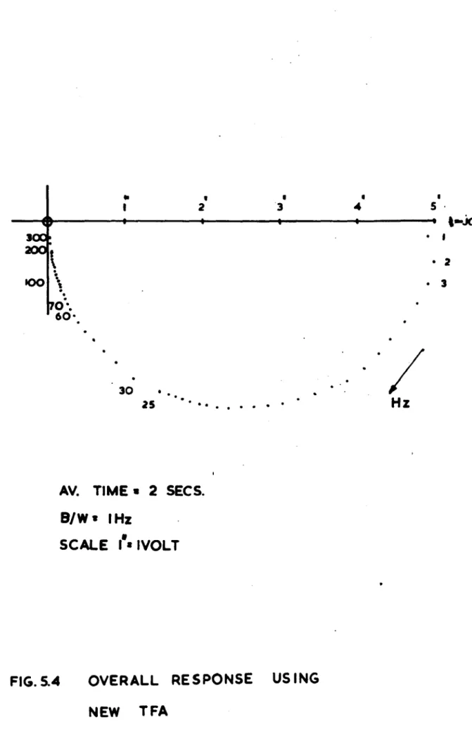
5.1

The Attenuators.

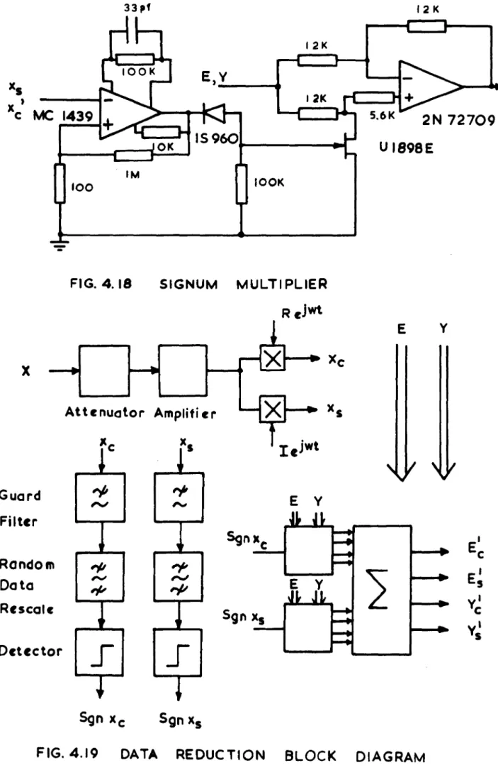
.signal Amplification • Signal Filtering. Signum Hultiplication.

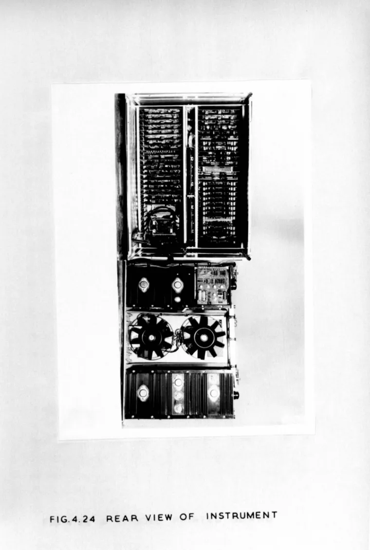
Analogue Data Processing. General Layout.

Figures

(4.1)

-

(4.25 ).

Performance of the Instrument. Introduction. Page.

63

63

64

65

66

67

68

5.2

Transient Behaviour of the

Adaptive Loop.

68

5.2.3

5.3

5.3.1

5.3.2

5.3.3

5.3.4

5.4

5.4.1

5.4.2

5.4.3

CHAPTER

6

6.1

References.

Use of a Single First-Order CRCF.

68

First-Order CRCF and Integrator. 70

Second-Order CRCF. 71

Experimental Results. 72

Bxperiments with Commercial TFA.

73

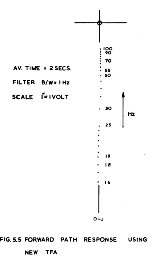
Deterministic Experiments with New TFA.

73

Random Data Experiments with New TFA. 75

Experiments on Real Systems. 76

Instrument Errors.

79

Commutating Filters.

79

True Multipliers. 82

Other Errors. 84

Figures (5.1) - (5.18) Conclusions.

Suggestions for Further Work. 86

88

CHAPTER TWO

A

Av( )

A

YX

b ( ) BT

B

yx

Cov [ ]

C (jw) ye

1 1 e itY f

e(t) f(l. )

m g('f )

G(jw)

h(c,- )

H(jw)

GLOSSARY OF PRINCIPAL SYMBOLS

Amplitude of signal.

Average or expected value ot.

Real part of true cross-spectral density function - S _yx •

Bias of.

Bandwidth - time product relating to the evaluation of co-variance matrix.

Imaginary part of true cross-spectral density function - S _yx •

Covariance of.

Estimate of cross-spectral density function - S _ye (jw).

Abbreviated notation for filtered portions of signals fed to the instrument.

lieul part of ~bove filtered signals. Imaginary part of above filtered signals.

Complex products obtained by multiplying

Error signal in feedback system. Scalar function of model err on

Impulse response of forward path. Fourier transform of g( '#) •

Impulse response of feedback path. Fourier transform of h(CT) •

Abbreviated notation for evuluation of integrals.

l~eal part of S / S •

K a L met) n net) q(cr )

H ('t')

ye

s

S (jw) ye

t

U m

Var ( )

V m w w c w e w o x(t) yet) z(t) Z,Y,X,Q,P,N,M

Gain of adaptive loop.

Imaginary part of S / S •

yx ex

Additive noise signal in feedback path. Integer.

Additive noise signal in forward path.

Impulse response of circuit between noise and output of forward path.

Impulse response of circuit between noise and output of feedback path.

Cross-correlation function between yet) and e(t) as a function of time delay.

Complex frequency variable in Laplacian notation. Fourier transform of R (1C) - true cross-spectral

ye density function.

Time variable.

Variables of integration.

Real part of model transfer function.

Variance of.

Imaginary part of model transfer function.

Frequency variable (radians per second) • Bandwidth of analysis filters.

"Equivalent bandwidth" of Heterodyning frequency.

Input signal. Output signal.

w •

c

Output signal from feedback path.

Abbreviated notation for Fourier transform of the respective time signals.

CHAPTER THREE

o ( t ) Modulating function. a ,a. ,b.

0 1 1

C C P f s Hz i,k iCt) K P met) q r R

s

_p

T u(t) v,V w a z

z

..I\.s

A

Fourier ooefficients of ~(t).

Capaoitanoe.

~eneralisation of cosine value at pth iteration.

Sampling frequenoy (oycles per second).

Discrete weight of OC(t).

Frequency. Integers. Current.

Generalisation of the weights of a digital counter.

Modulating function. Radix to power n. Radix.

Resistance.

th

Generalisation of sine value at p iteration.

Period of 0<. (t).

Heaviside step function. Voltages.

Analogue frequency variable.

Digital frequenoy variable.

Z transform variable. Impedance.

Error.

Angle.

1 -CHAPT~R ONE

Introduction

The thesis proposes to investigate a branch of control theory which deals with system identification. This topic may be

understood as an experimental attempt, by control engineers, to formulate the unknown behaviour of a controlled system in

mathematical terms or graphical displays. His objective usually stems from the desire to improve the performance of the system plant in question, when his knowledge may be limit~d through either

1) the plant being a new and untried piece of commercial hardware or

2) he not being fully conversant with all the system constants that he requires for his model.

The study must be observed in the time domain but the outcome of the identification may be realised in either the time or frequency domain. Choosing between the two, is a matter of personal

preference, depending on the ease and familiarity with which the display can be interpreted.

The experimental data may be the result of observing the response to closely defined inputs such as sinusoids and impulses. Unfortunately, industrial operations cannot always permit such

-2-normally. Collection of the data when the plant is running

normally, is given the title of "on-line II or "in-situ" measurements. However, if the system is stimulated by a stochastic or random, rather than deterministic signal, problems in the collection of data will arise. In particular, measurements will be time consuming, since consistent evaluation of the data can only be performed using averaging techniques. Due to this inherent time lag, immediate corrective action to the s~stem cannot be taken, it the random data analysis reveals an inadequate performance. In addition, the system must be linear and time - invariant, over at least the duration of the complete analysis, for the results to make senae.

The relative importance of the subject can be assessed by browsing through the contents of one IFAC Conference (Prague 1967). Papers by Cuenod and Sage (1) and E1khoff (2) give useful

introductions, whilst a recent comprehensive review has been provided by Balakrishnan (3). Identification techniques are

important not only to the control field. Communication systems

(4),

medical techniques

(5),

mechanical vibrations

(6),

oceanic (7) and atmospheric disturbanoes (8) all benefit from the same anal~sis. In each case, the problem may be generalised to estimating the _yst.m behaviour, when the measurement points are known to contain "additive noise".

The basio mathematical concepts involved were evaluated in the early part of this century but it was not until the work

ot

Rice (9) and Wiener (10). that the trvatment

ot

noise problems was firmly established. In this thesis, use of their techniques will be applied to the on-line estimation of frequency response functions in continuous torm.

1.1 aeview of Continuous Frequency Response Estimation using Computational Mothods.

-3-normal operating records originates from work carried out by

Goodman and Reswick (11). Although their approach was essentially based in the time domain using correlation studies, it revealed how modelling techniques could manipulate stationary second-order amplitude processes, to simulate an impulse response, evaluated at specific units of delay. Manipulation of the weights of a delay line were performed manually via visual comparison of the model and system cross-correlation functions. The frequency response followed naturally using Fourier transformation.

With the advent of spectral analysis in 1958, dynamic modelling was not to gain much favour after the initial impetus. Blackman and Tukey (12) rationalised the smoothing of time series by spectral methods, to show that computerised techniques could successfully eliminate all special purpose hardware, the "smoothing windows" and time-frequency transformations being implicit via the skill of the programmer. Concurrently, using the above methods, Goodman (13) developed a regression procedure for estimating the open-loop transfer function of a system when the driving and additive output noise disturbances were assumed uncorrelated. ~his method WclS

effectively the dual technique to (11). Goodman et al (14) successfully demonstrated the use of the former's approach, by applying stationary noise to simulated versions of a blending operation and a stirred tank reactor, to extract gain and phase information. Jenkins (15), without adding to the general theory, conducted similar experiments when evaluating the performance of a heat exchanger. A joint conclusion from these two papers appears to be, that conventional industrial plant self-generates insufficient uncorrelated disturbances of the input variables, to provide a

foundation for spectral analysis. Stanton (16,17) obtained vury useful results for turboalternator data, whilst attempting to

-4-instrumentation rather than insufficient data power.

Unfortunately, the above use of spectral techniques is

inapplicable for a system with feedback loops contaminated by noise. However, Akaike (18) showed that, excessive bias, in the

estimates for the feedback case, could be alleviated by referring

to a signal external to the control loop, which was uncorrelated with the stochastic disturbances. In doing so, he further

advanced the problem (19) of how best to make a two-point estimation of the forward path transfer function, when this reference signal was not present. The method relied upon "mixed spectra" whereby the output noise from the controller was assumed stationary and non-Gaussian, whereas the random disturbances and measurement errors were assumed to consist of traditional second-order statistics - a not very practical situation. It appears that this problem yet remains unsolved.

With the realisation of model-reference control systems (20), it was recognised that these techniques could be utilised for identification purposes. In particular, they are very useful (21) when updating

ot

the estimation is required due to time variations in the system. The method relies upon some "a priori" knowledge of the system order, expressed as a polynomial in the frequency do maiD , the polynomial coefficients being adjusted to minimise an error criterion between the system and model, usually based on gradient techniques. Both linear and non-linear systems with single-valued non-linearities (22) may be identified to advantage. In particular, use of analogue computer simulations, in combination with a suitable adjuetment algorithm can replace the costly

computing facilities required by spectral analysiS teChniques. 1.2 Review of Continuous,Freguencl Response Estimation using Special Purpose Hardware.

The techniques applied here tend to be sequential in nature, since

-5-schemes

facilities provided by a computer. The simplest are based upon

the injection of a sinusoidal stimulus into the system and the output response evaluated by correlation techniques, to remove

errors due to noise - a case of linear regression. Indeed,

resolution of the response into its constituent real and imaginary

portions, in combination with the above techniques, was used by Dwyer (23) for the construction of two differential equations for continuous single point estimation. When the equations reached their steady state, the response was directly interpreted as a measure of the syste~'s component gains. It was further claimed to evalu~te the system impulse response, at regular time intervals, when random data was used. However, unless use was made of

spectrum analysis, via evaluating the signal power content through narrow-bnnd filters, assuming knowledge of the i~put spectra to be "whiteli , _{very little progress had been made in this direction,}

until a paper was presented by Hughes and May (24). It revealed that, using analogue computer simulation, random data around a

specific region, could be extracted in blocks using filtering techniques, mnnipulnted by hardware in the form of a first-order

stochastic differential equation and in the steady state, produce reliable estimates of the system's real and imaginary gains. A hardware algorithm was baaed upon gr.adient techniques. The study was later to become the basis of a special purpose analyser for open-loop estimation

(25).

1.3 ~vation of Thesis.

Although analysis is possible and more practically viable in the time domain, this thesis aims to implement a special purpose instrument which will advance the approach to on-line estimation in

the frequency domain, with the presence of feedback loops. On-line correlators are commercially available but not for solving

-6-of a suitable stimulus, sinusoids, steps and impulses are -6-of

limited use, if there is an obvious desire not to upset the system, once it has been started. To this end, the intended hardware must

rely either upon injected random or pseudo - random data (26) or

on self-evident uncorrelated processes, naturally oocurring in the

oontrolled plant. However, it is worthwhile to note that, when

conditions are favourable, sinusoids do produce a high concentration of power in a very narrow bandwidth, so yielding robust estimates.

Applications would not be solely confined to identification of electrical and automatic control schemes. The instrument would be foreseen as invaluable to the whole field of frequency response analysis, which embraces random vibrations, biomedical applications and fluid mechanics. A consequence of its universal application in the engineering world would necessitate a design able to analyse

\''''~'I.",e:.I'\c:,e..s

frequences in a region as low as ·01Hz - for automatic control schemes - to 2KHZ, necessary for vibration analysis of machine tools. A corresponding amplitude range would involve orders of at least 60dB, in anyone sweep, with the possible addition of another 60dB of external scaling. Responses of any plant, tool joint etc., would be displayed using Nyquist plots. Since the instrument

would function, even if the plant input and output signals to it were interchanged, reciprocal identification is also feasible.

Arguments for such an instrument would find strong industrial appeal, due to the present limitation of current hardware. Indeed, applied sinusoids must corrupt the reference signal, giving rise to superimposed oscillation on the controlled output. Consequently, shut-down of the plant would appear inevitable, before a testing

-7-hardware which is unstable in the open-loop case e.g. integrators.

In this situation at present, known local feedback is administered

before correlators can be used with random data.

To summarise, it would appear that known methods of

identification are either too cumbersome, at present, to be of general industrial use, or cannot be used on-line in any feature.

Hence, the intended instrument should be a valu~ble contribution to dynamic analysis in the frequency domain, being both practical and uncomplicated by large-scale computing schemes, which tend, in consequence, to be of local academic interest.

1.4 Contribution of Thesis.

Chapter two initially deals with the mathematical background to the problom in general terms. It reveals that, an unbiased estimator of tho forward path transfer function may be obtained from a ratio of cross-spectra. In addition, a variance expression is deduced to reveal the effect of corrupting noise upon the

derived estimate. The chapter then continues by explaining, mathematically, how the available data may be manipulated by the method of gradients to form a two-parameter model estimate of the desired transfer function, evaluated at single points in the frequency domain. two first-order differential equations with stochastic coefficients are the outcome of the analysis. These may be solved in the mean, using a fourth-order integral expression. The parameter estimates are shown to converge exponentially and bias expressions are derived without recourse to the Fokker-Planck equation (25), in which the stochastic coefficients must be assumed macroscopically "white", in comparison to the averaging time of

the adaptive loop.

-8-i.e. information is processed in an analogue manner under the

influence of digital controls. Critical potentiometers are therefore no longer a source of concern for fr~quency sweeping. The

heterodyning technique is based upon a recursion, for the

trigonometrical functions sine and cosine, using identities similar to

:-sin (A+B)

=

sin A cos B + cos A sin B

sin (A+B+C)

=

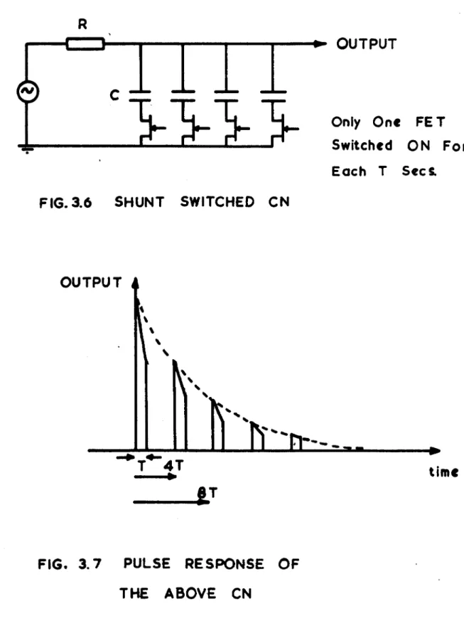
sin (A+B) cos C + cos(A+B) sin C This enables 3600 to be evaluated in 64 discrete steps, without using nearly the same amount of individual resistor weights.

Secondly, a new form of filter has been conceived by the

author, who is unaware of any other published reference to the topic.

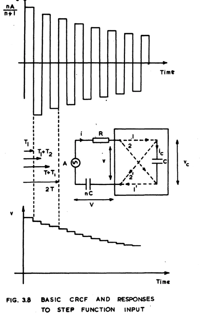
I t has been designated the "Capacitor Ratio Commutated Filter" (CRCF) and basically relies upon capacitors and switches for its construction. Such an arrangement can produce filters whose cut-off points are a function of the commutating frequency and the ratio

between the capacitors. In addition, these filters could theoretically be immune from temperature effects, if the capacitors have the same characteristics. This makes the technique feasible for integrated circuit manufacture. It is further revealed that, by recourse to

established active filter networks, similar characteristics can be obtained by replacing the fixed resistors by commutated capacitors, thus giving continuous variation of the cut-off frequency, without using either decade switched capacitors or variable resistors. Although only low-pass shapes have been analysed, certain features have been observed, which makes th~ author suspect that the technique could also be applied to both band-pass and high-pass filters.

-9-sweeping, heterodyning and filtering have all been locked to

digitally derived clock waveforms.

Chapter five illustrates the performance of the instrument in practice. It shows the results of identifying transfer functions in either closed-loop or open-loop systems, using an injected

sh~u.lu.s

stimulii based on sinusoids, pseudo-random sequences and Gaussian random data, the first two being implicitly derived test signals.

-10-CHAPTER TWO

Theoretical Study of a New Transfer Function Analyser 2.1 Introduction.

The previous chapter has highlighted the benefits and

requirements of a portable on-line random data analyser. Here, a

theoretical study reveals the fundamentals of such an instrument and illustrates the versatility of an adaptive loop to remove a practical drawback for low-signal-level transfer function analysis - that of division. In addition to developing the basic stochastic differential equations which govern the aforementioned loop,

approximate solutions for the bias and rate of convergence of the adaptive loop are derived.

Theoretical expressions «or the normalised variance of the real and imaginary portions of any forward path transfer function are derived. They reveal a strict dependency solely on the

coherence of the error path. 2.2 Basic Concepts.

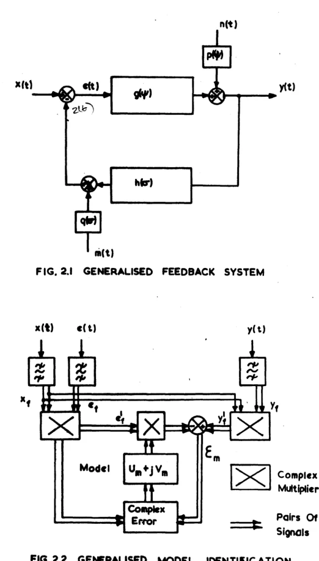
A schematic diagram is shown in Fig.(2.1). This depicts a

gen~ra1ised feedback system and the proposed instrument is intended to identify the forward or feedback transfer functions. The system

is observed to consist of a forward path network of impulse response g(~), the output of which is re-connected to the input via a feedback

network of impulse response h(er). Each network is assumed linear and time invariant, although not necessarily stable in the open-loop condition. The signals x(t). e(t). yet) are assumed to consist of statiQnary random variables. In addition, stochastic disturbances net), met) when passed through unknown linear networks of impulse

response p(~), q(cr) may interfere with measurements at the points indicated. The inputs net), met) are assumed to be additive noise sources, which are Gaussian with zero mean values and uncorre1ated

A "two-point" estimate of a transfer function is an estimate which is derived from two separate signals which are connected

-11-not necessarily assumed present. The problem, then, is to

measure either G(jw) or H(jw) - the fourier transforms of g(~),

hear) respectively - by applying spectral analysis techniques. No claim will be established for the use of the instrument

*

to solvE: the "two-point" feedback estimation problem posed by

Akaike (18) and Priestley (27), whereby x(t) ; 0, i.e. x(t) cannot in any way be reckoned as a source of information.

Consider first the time-domain approach.

yet)

=

f+~g('P)e(t-'II)d'f+

f+oO

p('f')n(t-V-)d'f

-OCJ -C/O

z( t)

=

I

+QO h(er )y( t-tT ) dO" +

J

+ cO q (cr )m( t- c:T)dcr

-00 -00

e(t)

=

x(t) - z(t)

It is thus observed that the various time functions are related by convolution integrals, whose lower limits will be zero if we consider conditions of physical realisability. These imply that the impulse responses g(~), h(er) are zero before the

application of a source at time t

=

O. In addition, it is assumed

that

,g('f)I,

tg(~)t2,

Ip('I'),'

I

p('f')t-2, Ih(C1")I,

t

h_(0")1 2_,

,q(cr)I, ,q(0")12, are integrable. Under these conditions, the equations (2.1) to (2.3) may be Fourier transformed into the frequency domain such that

Y(jw)

=

G(jw) E(jw) + p(jw) N(jw)

and similarly for Z(jw), E(jw), where w is the frequency in radians per second and the symbol j

=~.

(2.4)

Again viewing the approach in the time domain, it is possible to form correlation functions between the various signals. Such averaging techniques are required to reduce the corrupting effects of noise (11). If we consider e(t), yet) to be real variables, then it may be said that

-12-operator, R the cross-correlation function. This technique, which

is applied for the analysis of stable systems, when used in combination with (2.1) yields

Using the well-known one-to-one correspondence of correlation and spectral density functions, it may be stated that

S (jw)

=

S (jw) G(jw) + S (jw) P(jw)

ye ee ne

where S represents the double-sided spectral density function which may be real or complex. With stochastic signals, it is apparent that the forward path transfer function is readily identifiable as S (jw) or P(jw) tend to zero.

ne

2.2.1 Bias Aspects of Cross-Spectral Iduntification.

(2.6)

From (2.6), an estimate of the forward path transfer function may be obtained by saying

A

G (jw) =

c

(jw) - P (jw) C (jw) (2.7)

ye ne

C (jw) C (jw)

ee ee

where the circumflex indicates an estimator and C an approximation to the true spectral density S, by virtue of finite averaging.

"

The expected value of G (jw) will be unbiased if the signals net),

a(t) are uncorrelated and the ratio [Cye (jW>][Cee (jW)] -1 is

itself unbiased. One instance occurs when the feedback path is

open-circuited. Unfortunately, as aeen from Fig.(2.1), the interfering disturbance, net), must correlate with the error signal and thus

a biased estimate results. How may this be removed? From the notation developed for (2.4), using capital letters as an implied function of (jw), we may formally say

Y

=

GE + PN

2..8

•

•

•

-13-Z=HI+QM

E = X - (HI + QM) and (2.7) gives

:-Y

=

G [X - (RY + QM)] + PN

••• Y (1 + GH) = GX - GQM + PN

Similarly

E (1 + GH)

=

X - HPN - QM

(2.12)

Let us take an information point external to the loop, s~y X

and disregard the effects of non-ideal filtering of the data. Therefore

•

••

from (2.12) and (2.13)

1-C _yx

=

G C _xx - GQC _mx + PC _we

-1 +GH 1 +GH 1+GH

C ₌ C HPC _{- QC}

ex _~ we _-.m!.

1+GH 1+GH 1+GH

Cy y

=

GO - GQC + PC

... xx mx nx

c

_ex C _xx - HPC _nx - QC _mx

(2.14)

(2.15)

Hence, from the initially assumed zero correlation between the disturbances and the random signal x(t), the estimate, after ensemble averaging of both numerator and denominator yields

S

=

G ...l!

S

ex

and an unbiased result is obtained. A variance component will of

course remain. !kaike (18) has in fact suggested that, viewing of the signal external to the loop is not a necessary prerequisite for an unbiased estimate. All that is required, is information which correlates with this reference signal. The instrument,

described in this thesis, will exploit this fact to simplify its operation.

From (2.8) to (2.13) the equivalent spectral density equations result

:-=

fGI

2

I

p 12

•

•

C C_ee +

_°nn

+00 P + P C G _(2.18)

yy en ne

0 • 0

-

HC _{- QC}

(2.19)

en xn yn mn

Cyn aGe +PC

(2.20)

en nn

where the asterisk signifies a complex conjugate.

Making use of (2.7) an estimate of the bias yiel48

:-POne

-[0

_ tGI

2

0

.. tpt

2 C - 00 PJ

'U. ee nn en

•

0 C G

ee ee

!y taking expected values throughout, it can be seen that

•

See G

assuming

x,

m, n are all mutually uncorrelated and b symbolises the bias term. The value of the bias can be made equal to zero, either when no noise sour~ net) is present, or the feedback loop

is open-circuited. An interesting sidelight of (2.21) further reveals that although introduotion of the feedback noise source, m(t), inflates S and S , i t cannot affect the bias term when

yy ee

Snn

=

0. For this situation, S .. = fG

12

S and therefore b

[~J

=0.

yy " ee

Using a similar derivation of the result in (2.16), an unbiased estimator of

H

could be obtained by using the ratio

( Ozx) ( C"". ) -1. ~_ If the est mator was obta ned uS1ng on y i i · 1 th e signals z(t), yet), an equivalent bias term to (2.21) would prevail, except that the expression would be influenced more by

"

m(t), due to the effective roles of met) and net) being interchanged in the nnalysis.

2.2.2 Variance Aspects of Oross-Spectral Identification.

"

-15-"

instrument, the value of G is required in orthogonal co-ordinates such that

"

K _ Real part of C / C

yx ex

"

L • Quadrature part of C / C

yx ex

and C ,C can be split into co and quadrature spectral 1X ex

A ,.

density components

A, B

respectively.

"

."

,.."

: . K - A A +B B

yx ex yx ex A 2

A

ex + ~ ex 2 It " 1 \ " "

L • A

_1X

B

_ex

- A Bvv

_ex

,,-"2

+ B _ex

:I: RP C C

yx ex

c

C

ex ex

•

•

II 1m

pee

yx ex

"

"

•

•

(2.22)

Now consider small perturbations

bA, SB

about the expected or average value".

Av

(~]

_•

At

Av

(iJ

a

B

so that

"

'"

Ayx

-

A

_1X

+ iA

yx

"

_BiX

_•

B

+iB

,...

'1X

yx

"

A

Aex

•

A _ex

+SA

ex

~

_"

Bex

-

B

ex +~B ex Further

define:-Av

[~A1X]

•

Av

[S

~yx]

•

AV[~ ~ex]

• AV[&Bex] •

0

Av

['A:X] •

Vnr

(Ayx]

AVrSA1X

5~]

•

Cov

(~1X'

;yx]

etc.

Hence, A

K •

+~;

)]

ex

(2.24)

~

• [<A

+,

A )

(B +

S: ) -

(A

+, : )

(B

+s~

)l

yx :IX ex ex ex ex:IX 1X

J

+

A Taylor series expansion of a non-linear funotion g(X 1 ,X

2 ,X, •••• Xn) of random variables (X1 ,X2

,X, •••

Xn) may be written about the point (0.1,a

2,a, ••• an)

as:-g(X1 ,X2

,x

3 •• X .... )

z

g("1'''2'''3 •• ..,,)

t

~

[fiJ

(Xi - "i) Xi • ai (2.26) ~

This is performed in Appena~One for K and due to the

A

similarity between (2.24) and (2.25), inferred for L. Consequently, it is observed from (Al.3) and (A1.?) that

Av

[~J

Ay

[~]

=

Re Part S S

yx ex

s

S

ex ex

• 1m Part S S

yx ex S _{ex ex} S

•

•

•

•

a~::::

"r1 - 11

L

;;;Lii

J

(2.28)

where

Jib,.

(A1.8) is the ooherency function,..a real number such that OE

~i ~

1 - and is defined by Enoohson (29). It direotly gives a Mensure of signal/noise power ratio at the measurement pOints e and x. When no noise is present, there is no variance in the estimates of K and L. Goodman's (13) work on the open-loop estimate resulted in confidence expressions depending onlf. It would be interesting to find out whether

1

i

and

1

f

are

-17-Using

(2.12

to

2.15)

it can be

snid:-C

TI

I

1

+ GU

,2

II

I

GI

2

_c

xx +

'GQ 1

2

_c

mm +

I

pi

2C

nn

-IGI

2

_Q·C

xm

+ Gp·c

xn

-lGI

2

QCmx - GQp·Cmn

•

•

•

+GPC -

PGQC

we nm

Taking expected values of

(2.30)

assuming x,m,n to be mutually uncorrelated

Also

•

•

•

- H P C_{xn -} Q 0xm

•

- HPC _nx +HPQC _nm

- QC mx +

QH P C

•

•

mn

Hence, by expected

values:-See

I

1 +

QUl

2 • Sxx +

IBPI

2Snn +

IQI

2Smm

• I

Gt

2s

!x

11

+ GHI2

1.

2

'XX

•

'1 .

Gul

2

Using

(2.31)

to

(2.35)

"§ •

'S7XI~

•

( 1

G 12sxx +

J

GQI

2smm +

I pI

2snn ) Su

• s2zx

(2.37)

(sxx +

I

QI2Smm

+

t

HP

1

2S

nn) Su

the error ~that ot the output, stems from a desire to circumvent the necessity for evaluating the probability density distributions

ot the required estimators. If these coherency functions in the

closed-loop case are identical, an equivalent open-loop model may be derived for the closed-loop system. Use may then be made ot

Goodman's work to evaluate the confidence intervals tor the estimators. Wellstead (,0) pursued this approach when trying to identity the magnitude and pbaae of a torward path transfer

tunction, using Smm • 0 and

IHI2 •

1. Equations (2.36) and (2.37) agree with his analysis but also reveal that it may'be further advanced to cope with feedback noise as well, with the proviso that either

fBt

2 D 1 or S

.0.

No further attempt will be made

nn

in this thesis to develop the necessary confidence intervals,

since much experimental data would be necessary to justify the theory.

2.'

An

Adaptive Modelling TeChnique.

The technique relies upon the fact that the response of a linear time-invariant system to a complex exponential stimulus, results in an output which is characterised both by the system resolved gain taotors, in the frequency domain and the resolved compoaeats of the input signal. Thus, if the input is ot the

torm .(t) • Ae3wt • the steady-state output will be

yet) • A (cos wt + j sin wt) [U(w) •

jV(~)]

(2.}8) where I(w) and yew) are the real and imaginary portions ot G(jw)

respeotively.

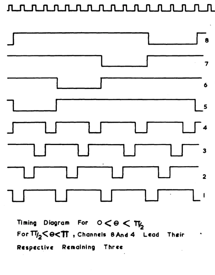
If we refer to Fig. (2.2) and assume the effective value of x(t) temporarily: 1, the signal e(t) may be resolved and the separate components applied to a two dimensional model of the system, evaluated at a partioular frequency and the resultant output compared with that of the true system. An error measure Em will r .. ult, which may be used, automatically, to adjust the gain model parameters, suoh that the model [;m(w,t) +

j~m(w.t)]

-19-error criterion. Dwyer (23) arrived at this techni~ue via

regression analysis for the special case of sinusoidal data and zero feedback. It is to be noted that the model will be obtained

using point-to-point plotting in the frequency domain and hence is necessarily time consuming. This would appear to be the price to pay, if one requires portability. Otherwise, with storage

techni~ues. a polynomial model, expressed in the "s-plane", would have been ideal, although requiring more than two parameters to be optimised. These have already been discussed in Chapter One, where it was observed that such techniques require extensive computational facilities.

If we are to apply the above techni~ua to modelling the response of a system to random data, the signals from the system will initially, have to be accurately filtered. This necessity

•

stems from Ric~ (9) representation of random data, as a finite sum of sinusoids, whose fre~uencies are multiples of a fre~uency,

wn and related to the duration of the analysis. Consequently, a signal of very low power content would be the result of trying to analyse anyone particular fre~uency. Therefore, in accordance with recognised techni~ues of power spectral estimation C1), an assessment of the average power is taken by viewing adjacent

fre~uency components in addition to the component of interest. The assumption is made,that the spectral densities of these surrounding components are "white". Filtering is therefore required, the merits and practical realisation of which will be covered in Chapter Three. Meanwhile, it remains to state that after resolving the data, it has been thought better to manipulate

the signal around zero fre~uency and hence the filter structures will be of the low-pass variety and not directly band-pass, as illustrated in Fig. (2.2).

2.3.1 Parnmeter Adjustment.

-20-hill-climbing, is known as the method of gradients. This permits

parameter adjustments to be made, which are pr9portional to the local gradient of a suitable error function. The technique appears to have advanced from studies at M.I.T.(20). In context, let us

use the symbols

:-f(~) to denote a scalar function of the error between

the system resolved outputs and those of the

!m(W,tl }

V (w,t) m

model.

to denote estimates of the model gains U(w), yew) respectively.

K

a to denote the gain of each adaptive loop.

1\

-1Ka~f[em(tB

Therefore, dU (w,t) _m =

2

"

dt

)u

(w,t)

m

'"

_Ka~f

_[f

_m(t8

dV (w,t) _{= - 1}

m (2.40)

dt 2

~V

(w,t)

m

From now onwards, explicit use of the independent variables w,t will be dropped when the text is not ambiguous.

Referring to (2.17),

s

=

(U + • V )

s

yx m J m ex (2.41)

is the result which we hope to instrument, based upon the error function

If

12 =

e.

E...

This composition of error variables has

m m m

been shown by May (25) to result in a set of linear equations with stochastic coefficients. Equation (2.41) implies that the input signal to the model must be a complex function of the signals

e and x, with the complementary output being a similar complex function of y and x. The generalised diagram of Fig.(2.2) may

now be fully symbolised as follows. Consider each of the signals x,e,y to be resolved and filtered such that

X

f

=

x C + jx s

=

(2.42)

where the subscript f implies filtered data

where the subscript c implies in-phase component relative to

an

arbitrary clock reference.

where the subscript s implies quadrature-phase component. Since x_f •

further define Therefore

e

_rt

Y

f are inputs to complex multipliers, we -&1 e1 f and '11

t

to consiat t also, of pairs of signals.

e1

=

e1 + je1

f tc fa

• (e_c + jes)(x_c + jx_{s )}

• (. x _{c c - ex) a s} +j (esxc + ex) _{c 8}

'11 _{= y} 1 _fc + jy1

t ta

• (y _c + j" ) _s (x _c + jx ) _a

• (1'

_c

x -_C Y _{8 S} x ) + j (YaXc + "cxs)

Referring to the parameter adjustment equations

(2.39), (2.40)

d;

= -

~

[-f

m e

1

r • -

f

m• e

1]

(2.47)

d:

c:

d:: ·

-1 [

3t;. .\. -

3~· .~

]

(2.48)

Since j«(me1f·) •

j~

••

e~

>:

equations

(2.47), (2.48)

can

be further simplified to the following

torms.

81m11&1\1

d~m

• Ka Real.[£m·

e~]

dt

"

dV II

dt

• Ka [Eiae .1 te

+

E ....

1 ta ]

• jKa

Imag[E m·

e1

rJ

& Ka

[e""

.1 fa

-E .... •

1 fa ] (2.50)

-22-further determine the manner of convergence of the estimates of

the parameters U and V. Unfortunately, the arrangement is not _{m m} conducive to forming ~. impression of the convergence in terms of the stimulating random signals. This may be accomplished by substituting forE as

follows;-• m

"

Ka [ (7 1

fe 1

-1

,..

1 A 1

J

U = _{e fc} U _{+ e fs Vm) e fc}

m m

1

"

1 i\ 1 + (y fs _{e fs} U _{- e f V) e fs}

•

m c m

"

Ka[y1fc 1 1 1

"

(e1 2 1 2ry

i.e. U 1:1

e fc + y fs e fs - U + e fs)

m m fc

(2.51) In passing, it is worthwhile to note for future reference that

1 1 1 1 [ ]

Y fc e fc + Y f e f C

i

(y +jy )(e -je )+(e +je )(y -jy )

8 s C s e s c s c s

2 2

x (xs + xc' (2.52)

1 1 1\ 1 2 1 2;1

- Y fc e fs - VmCe fc + e fS)J (2.53) where the dot notation indicates differentiation with respect to time. Hence two first-order linear differential equations with stochastic coefficients have resulted. These, together with the complex notation developed in this section, completely define the organisation of the parameter adjustment loops and the

arrangement is depicted in Fig. (2.3), in which the synchrodyning waveform is taken to be of unit amplitude.

-23-averaging but should be independent of signal levels. It would

greatly simplify the organisation of the instrument, if the respoUtie time of the adaptive loops was also independent of signal levels. Unfortunately, since stochastic differential oquations are involved,

" 1\

the analysis may be awkward, especially since U ,V are non-_{m m} stationary random functions. In consequence, an approximate solution is advanced, which assumes sufficient degrees of freedom present in the averaging circuits, such that the model gains and the stochastic coefficients can be considered independent. The resultant answers produce no less insight of the exact solution, than had recourse been made to a simulation based upon the

Fokker-Planck equation (25). The reason for this, is due to the implioit requirements of the Fokker-Planck equation to have its stochastic coefficients macroscopically "white", in comparison to the model gains. One extra condition, not highlighted in (25), is that the extent of the "white8ess" must be expressly interpreted from the problem. This is of paramount importance, since an infinite noise spectrum must be treated differently to the band-limited case.

An

excellent discussion of the matter has been given in a paper by Caughey and Dienes (32).

For the approximate solution, a feature of the mathematics will be the requirement to evaluate integrals of a fourth-order moment.

2.4.1.

An

Approximation to the Mean Solution of the Model Gains. Let us take equation (2.51) as an example and view the

Heneea

-~

iii (

[11

ID 0. tc

.1

te + l ' e

1

_~

(e1

₂

_{+ e}1

₂

)1

fs fs m fc fs

J

where the bar signifies ensemble averaging.

In the steady state, the solution must therefore tend towards

Av [ ; mJ • _A_V_[y ___ 1 f;;.e __ e ___ 1 f;;.O ___

+~1~1

... f_S __ e_1 ... f;,;;;SJ-J

Av [e

1

_f0

2

+ . i

_ts

'J

Similarly,

Av [ Om]

=

Av

[1

1 fs e 1 fc - Y 1 fc e 1 fS]

r1 2 1 2J

Av

L

e fo + e f. .

From both (2.55) and (2.56) the estimate of the model parameters, in the mean, is shown to depend on moments of a fourth-order process. A typical expression can be generalised to one of evaluating the f~h-order moment of the signals

[a';tbftO;tdf] , where af "

'!,

of' df , are outcomes of the process generated via the heterodyning and filter operations •

. . pjw_o(t-u₁) h(u₁) dU1 represents the via a complex exponential of frequency

w

_o

radians per second and eonvol,.d with a low-pass filter of impulse response h(U

1

>.

Consequently,

Taking expected values of the above equations, results in moments of a fourth-order integrand oonsisting of Gaussian

prooesses. By manipulation of the variables and changes in the order of integration, an evaluation in Appendix Three leaves the

that&-where 8_ij is the double-sided power spectral density function of the respective signals and H(jw) the Fourier transform of h(u).

At first sight, the above expression would appear to be rather involved in comparison to the original equation (2.57). However, after a moment's deliberation over Fig. (2.4), the composition 1

1(U),I2(U),I3(U) visually illustrates how simple

the final result will become. In.Jig.(2.4), the filter transfer functions H

1(jw),H2(jw),H3(jw}Jl4(jW) are taken to be identical

-a pr-actic-al result of requiring six very closely controlled d-at-a reduction channels. In addition, they are illustrated as having perfect attenuation beyond the cut-off point

w

=

w •

c

Therefore,

Av (a.;bfC;df]!:::::....l..

4n

2

assuming the relevent power spectral density functions to

be virtually constant and w - W

>

Q,

o c

Dividing throughout by the product of the two integrals, each defined by both Bendat and Piersol (33 ) and Jenkins and Watts

(34 )

as "the equivalent bandwidth- of the data filters, we are

left, in the limit as w~ 0 with an estimate which reduces to

c

the product of the power spectral densities of the relevant signals at the heterodyning frequency w , as 8 dew )8 b(w ). _o

-26-Hence, we may now revert to (2.55) and (2.56) to discuss the

evaluation of Av

[~m1

' Av

[~m]

• Quantities of interest

are:-~

e1 +y1 e1

=

i

r(y +jy )(e -je )+(e +je )(y -jy )] [x2+x2] (2.61) . fc fc fs fa ~ c a c s c s c s c s

';se;c· '

;ce;s •

i

[(lc+jYs)(ec·jea>-(ec+jes)(yc-jys»

x~xc+jXs,)·

_(Xc·jxs

>]

•

_[ (e _c +je )(e .je )(x +jx )ex -jx _{s c s c s c s}

>]

SUbstitution of (2.61) and (2.63) into (2.55) yields

"

Av rUm] •

i

Av [Xf·efYf·xf + xf·Yfef·xf]

,.. AT

[7o

_{t '}

e

_t

a/x

_{f ]}

:. Av [U_{m] •}

i

[Syx

Sxe + Sex

Szy]

S _ex S

xe

assuming the effective bandwidths of the data channels to be well matched and their heterodyned power spectral density functions to be virtually constant, over the bandwidths of the filters as w

-+

o.

c

i.e. Av

[~m]

= Real Part of S _{yx ex} S

•

•

S S ex ex

which will be remembered as the desired theoretical result of (2.27).

Similarly, Av

(~m]

• Imag Part of 81% Se: (2.66)

•

S 8 ex ex

which itself corresponds to (2.28) and consequently, an on-line transfer function analyser operating on random data has been, at least, theoretically synthesised.

2.4.2 An Approximate Discussion of Bias.

epectral density functions - and this may be controlled by astute

selection of filters - a virtually unbiased estimate of the analysed transfer function must be so obtained. Unfortunately. referring to the joint integral leU) (2.59) and Fig.(2.4), it

is observed that further terms in the expectation will be involved,

namely when w ~ w. From Fig. (2.4)(c,d,e,f), the spectral

0 ' c

windows H(jw), H(jw -j2w ) will begin to overlap, adding additional _o terms to both numerator and denominator. Therefore, both cross-spectral est~es will be themselves seperately biased,

irrespective of how narrow is the filter bandwidth. In the case of perfect attenuation, the analysis for a strictly unbiased estimate, assuming w to be narrow, is confined to the region

c

w

>

w. Imperfect filtering will, however, produce a "tail" to o c

the filter responses and it is suggested that a safety factor equivalent to w ~

iv

should be emplo.-4. For a spectral

cA' 0

window consisting of two second-order Butterworth structures in cascade, approximately 20dB of attenuation will have occurred in each spectral window, before interaction takes place, if the latter : lDequality is satisfied.

2.4.3 An Approximate Discussion of Convergence.

A

;..

The expressions for U and V could not be originally

m m

evaluated, since the coefficients were stochastic. However, by taking expected values, a deterministic orientation, in terms of

menn values, remains to be solved using standard techniques

applicable to equations with consta.nt coefficients. To simplify matters,

w.

will be the "equivalent bandwidth" and for the

instrument, corresponds to two second-order Butterworth structures

in cascade. Tables of standard integrals are reproduced in

Shinners' book (35 ) and in Appendix Four, the resultant value of

:-

-28-~

.. (a,WO)

G

+

KaV.~

Is.,,:l

2

J

c ;m(O}+[ KawoiSyx

Se;]

/ e

(2.67)

~ A

U (0) is the previous evaluation of U i.e. at (w-w

+S'

w )

m m o o

-"

=

~

(O,w -6w ) m o o

U (0) thus indicates the "a priori" knowledge of the previous m

estimate at (w - , w ), where w is the present heterodyning 0 0 0

frequency. Inverse transformation of (2.67) and using partial

-

,..

fractions, it is readily apparent that U (w ) tends towards the

m 0 real part of S JS according

%

yr

ex to 1- exp [- Kawe2 fSexJ

2~

• Likewise, V (w ) will converge _m

0 to the imaginary part of S y)( JS ex •

Therefore, the time constant of adaptation depends on both signal power and averaging parameters. One source of error depends upon the filtered channels being well matched. If this is not so,

-

-A ~ 2

then Um(w_o)' Vm(w_o) are each inflated according to (w_e1/w_e2) • One final point to notice, stems from the solution of (2.67) • •

1\

U (0) _m will decay exponentially, according to the time constant

f a

W~2

Isex 1

2

J

-1 .econcla. Hence, the previous knowledge of

~

m o o (w

-~w)

cannot be used in any way to speed up the convergonce _ _

to the final value of

~

(w ), since

U

(w -£w) will, by then,

m o m 0 0

have decayed to zero.

this chapter has revealed the theoretical basis of a practical transfer function analyser, suitable for the on-line analysis of random data. Sufficient equations ha.e been developed to show that the instrument could be simulated, if desired, on an

net)

xrtl

c(t)

_yet)

x

Ii(t)

FIG. 2.1 GENERALISED FEEDBACK SYSTEM

x(t)

c( ~)

_yet)

!

1

.

.~.

Z

:t

_,--~

"/I " , , ,.."

•

f Lo, _~

_e.

~

•.

"

I

.1Ot-

y~

X

cf _

..

X

...

...

_X

ft

_Em

Model

_U.+jV.

[gJ

tt

-

CoMplex

~

-.::

_Error

c:

....

r-Complex

Multiplicr

Pairs

Of

Signals

Flct 2.2 GENERALISED

MODEL IDENTifiCATION

"nwt

Low

Pas.

Filtc r

e'

_f.

x

xlt)

coswt

x ... x

x

x

x

x

'~c

Multiplication

•

•

c

_{f •}

Addition

fmc

ems

e(t)

_Y(t)

.in~

x ...

x

_x

--Multiplica-&

tion

i

i

n

I

Yfs

FIG.2.3 AN ADAPTIVE LOOP TRANSFER

FUNCTION ANALYSER

·--2w

o

w·O

!c

•

~

, Sed(W"""",

- I

I~

\ (a

l •

-

w

_x

•

,

W

I I

\ ( b l

So"''''''''''

/

•

"

1,(U)

I I

,

I

.

I

H(Jw-j

_{H(jw) : \}

I _I

I

,

,

_•

\

Il=)

Sbr-W~

_x

"/

x

I

•

'aJ-07

,

\

Idl

x

I

I (U)

I

I

₂

I

•

I I

I

I

Saroi

I

\

Ie)'

I

x

,

I \

S~~i

I

\~I

.

_x

-29-CHAPTER THREE

NOVEL ELECTRONIC FILTERING TECHNIQUES

,.1

Introduction

This chapter has been isolated from a discussion of the

complete instrument, since new methods of tracking and filtering of the observed random data are claimed. These include a

superior form of heterodyning, based on recursion techniques, as compared to R. May (25) and a revolutionary form of filter, which rel~es upon commutating techniques. The chapter is split into two parts. The first, based upon the heterodyning operation,

... sises how such a modulator may be controlled by digital techniques to produce an analogue circuit of high accuracy and repeatability. Resolution of the data into two components phase displaced by IT/2 radians results. The latter part illustrates the filtering operation upon such resolved data. Use again, is made of digitally controlled networks, since six identical channels must be aligned, regarding both amplitude and phase characteristics. Resultant performance allows the alignment to

!

1% again yielding continuous repeatability.

3.2

Aspects of the Resolver.

The instrument must be capable of identifying all the available frequenCies, the tracking time being bounded by the instrument's natural response or the statistical estimation time, whichever is the greater. A scheme of identification must either

:-a) Track Simultaneously each of the frequencies stimulating the system or

b) Translate them to a specific narrowly defined band, where they will be viewed to the best advantage and appropriately

analysed. The merits of the two techniques using narrow-band responses have been well analysed in the literature

(36,37).

:-

-30-a) Analogue real-time analysis requires multiple filters for

speotrum estimation. However, the expense of combing the spectrum

up to 2KHs using bandwidths of 1Hz would be prohibitive. Further, high resolution -required for independent samples- is impraotical

due to imperfect out-ol-band attenuation. In addition, the requirement for progressively higher tlQtI tuned filters, when

analysing constant increments of frequenc~ completely eliminates this technique for the instrument.

b) Heterodyning is the principle of modulating a known sinusoidal carrier by an arbitrary signal, such that the desired spectral portion, centred around the carrier frequency, is translated to a fixed narrow band-pass filter region, where the information is extracted. Sometimes, recording of the original sample together with repeated playback is used but in any case, real-time analysis is not possible due to the sequencing properties of the heterodyne. A distinct advantage arises, however, in that the sequencing

properties will precipitate a more sophisticated design of the single filter, in comparison to the fixed bandwidths usual in the real-time analysis.

For the application under consideration, the modulated carrier will be of the same frequency as the signal component being analysed. This component will now be available at zero and dOUble frequency and oonsequently, synchronous demodulation should be taken as a more descriptive term for the process. Estimates of the power spectral density properties are readily obtainable from the d.c. terms. This is preferable to using the dou'le frequency sideband since

:-a) Extra circuitry is required to seperate the in-phase and

quadrature phased oomponents.