Aspects of self adaptive control using parameter perturbation techniques

University of Warwick institutional repository:

http://go.warwick.ac.uk/wrap

A Thesis Submitted for the Degree of PhD at the University of Warwick

http://go.warwick.ac.uk/wrap/61725

This thesis is made available online and is protected by original copyright.

Please scroll down to view the document itself.

ASPECTS

QE

SELF-ADAPTIVE CONTROL

USING

PARAMETER

PERTURBATION

TECHNIQUES

by A.J.R. Pawley, B.A. (Oxon)

April

1969

...

,

BEST COpy

.

,

•

, .AVAILABLE'

.

(1)

ABSTRACT

ASPECTS

OF SELF-ADAPTIVE

CONTROL USING

PARAMETER

PERTURBATION

TECHNIQUES

This thesis is concerned with the performance

of a method of

simultaneous identification and optimization of a control system,

employing a parameter perturbation techniQue.

The work is divided into four parts:

(i)

The evaluation of several techniQues for the identification

and gain-estimation

of plants having one "input" and one

"output", in the presence of noise, where the "input is a

controllable parameter, and the "output" is a criterion of

the cost of the plant, which is some function of the plant

variables.

The slope of the cost-function

is then given

by the "gain" of

¥'El

plant.

(ii)

The optimization of plants having more than one dynamic

path between input and output.

(iii)

The optimization of multi-parameter

plants.

(iv)

A general consideration

of optimization strategies.

The first part of the thesis is based on the well known

technique of obtaining the step response of a plant by applying a

pse~do-random binary seQuence (or "chain-code") at the input,

cross-correlating this with the ou.tput, and integrating.

A techniQue

equival~nt to this, using a multiplier

and running-averager,

is

(1i)

identification process are chosen so as to reduce the variance of the

gain-estimate to a minimum, the error due to d.c.-bias may be large.

Practical results are given, which support the theory.

An alternative scheme is considered which enables the d.c.

eDTor to be effectively removed.

Various methods of implementing

this scheme in practice are proposed for use with and without a digital

process-control computer.

The scheme is analysed under the same noise

conditions as before.

The signal and noise components of the

gain-estimate are evaluated in terms of the parameters of the system, and a

design procedure for the choice of optimal values for these parameters

is formulated.

A method of gain-estimation using sine-wave perturbations

is then analysed under similar noise conditions, and compared with the

Chain-code method.

The second part of the work is devoted to the optimization of

plants having more than one dynamic path between input and output, with

a different cost-functi.on in each path.

It is shown that the estimated

position of the optimum varies with perturbation frequency when using

sine-wave perturbation,

l!!§il'OOA teo tpue epHHllJ'ffl ~

s

femld T.vlssl'

ned~

ot'

chain-cod.es.

The theory is supported by the experimental anaIyad.s of

a simplified model based on a steam-generating plant.

In the third part, various methods of identification of

multi-channel plants are conSidered, based on the use of chain-codes.

The

extent of croBs-coupling between channels is examined, and ways of

reducing this are evaluated.

It is found that the best solution

],S

to

use time-shifted versions of the same chain-code, applied to the different

inputs of the plante

Practical methods of implementing this are discussed,

and a multi-channel optimization program is built up for use with an

(ii

i)

without compensation

for the effect that previous changes in parameter

have on the estimate of the gradient of the cost-function.

In the last part of the thesis, the basic limitations on speed

of pptimizaUon

a+,e inve!:)tigated.

Various strategies for rapid

hill-climbing are discussed, and a technique

for minimizing the number of

optimization

steps ~s developed •

( tv)

ACKNOWLEDGEMENTS

The work described in this thesis was carried out at the

University

of Warwick from October

1965

until September

1968,

under

a Science Research Council Research Studentship

grant.

LIST OF SYMBOLS

Certain symbols used only locally are not listed here.

In some cases they duplicate the symbols below, but the local

definitions make the meanings clear.

The last column below

indicates the sections in which the symbols are defined.

§¥!nbol

a a s

A

n B

c( t)

c .(

t)

J C C a

et

d d e

Definition

chain-code amplitude scale factor

amplitude of sine-wa~e

amplitude of Fou~ier components of m

scaled-expression

for variance

unit chain-code (amplitude

=

±1)

j-th chain-code in multi-parameter

system

co-variance function

cost of aotions applied to a system

cost index for a process at time t

vector of disturbances

error in d.c. estimate

D

standard deviation of gain estimate using chain-code

D Cl D s D z

E [ ]

f(K)

f

j(K)

fN

fs

t;v

and d.c. compensation

scaled version of D

s

standard deviation of gain estimate using chain-code

and no doco compensation

standard deviation of gain estimate using sine-wave

expected value of bracketed

terms

performance

function of single-path plant

performance

function of j-th parallel path

normalized frequency of·sine-wa.ve

frequency of sine-wave

double-integral

used in evaluating D2

( v)

Section

2.2 5.2

2.4(a)

2.4(b)

2.2 .

7.2

4·5

1.

2( b)

1.2(b)

1.

2( a)

4.4(

a)

2.4(a)

5. 3(

a)

4.2

6.

2(

a)

6.

2(

a)

6. 3(

b)

Symbol

f(19 f1(19 ft

(10

Fj

F(w)

Definition

function relating Pt to ~

function ~elating Ca to k

fUnction relating Vt to k

value of

F(w)

for j-th parallel path

ratio of gain estimate to true gain using sine-wave

true gain

estimate of gain using chain-code

total error in estimate of gain

gain error due to periodicity

gain error due to d.c. bias estimation

gain error due to non~finite plant settling time

estimate of gain

u·sing

sine-wave

(~)t

slope of performanoe function in i-th direction

at time

·t

h( "t)

h(-r, t)

hj(

e)

/\

hj(a)

AI

hj(s)

hr("'t)

Hr(

jW)

[H]

1-f[ ]

i

k

impulse response of plant

time-dependent

impulse response of plant

impulse response of j-th parallel path

primary estimate of h.(s)

J

secondary estimate of hj(s)

impulse response of running summer

power spectrum of running averager

mat'rix of transfer functions

Heaviside function

(=0

if

[J~

0, .. [ ] otherwise)

vector of intermediate variables of process

number of bits averaged for d.c. estimation

vector of plant parameters

i-th parameter of plant

plant parameter

(vi)

Section

1. 2( b) 1.2(b)

1.2(b)

6. 2( a)

5.2

4.4( a)

4.4( a)

4.4( a)

4.4( a)

4.4(a)

4.4(a)

5.2

1.2(b) 2.2 2.2

6. 2( a)

7.3

7.3

A2.2

A2.2

1.2'a)

4.3(

a)

1. 2(

a)

3.2

1.

2( a)

Symbol

K e K n K o K

opt

/\ K

opt

n c n o p

Pi

Pq_

P(t)'P

t A p(

t)

q( t)

q_av(t)

q, ~

(t)

r( t)

R R s

$ (w)

e

(vii)

Definition

error in estimate of K

_op

t

value of

K

at n-th clock time

10.2

present value of

K 1.2(

c)

6.3(b)

6. 3(b)

opti.mum value of

K

estimated value of

K

t

op

number of test steps/operative

step

1.4

2.

3( a)

2.4( a)

7.4

1. 2( b)

8.3

output of multiplier

noise component of output of multiplier

number of bits in a chain-code

(*N)

number of parameters

of plant

ordinate at start of q_-th impulse response

number of shift-register

stages

ALI

ordinate of impulse response reduced to zero

4.4(b)

4.4(b)

7.4

2.3(a)

6.2(a)

8.3

first zero-crossing

of impulse response

number of ohannels of system

number of bits corresponding

to T

r

output of i-th performance

function

ordinate of step response

6f q_-th ohannel

performance

index at time t

1.2

estimate of pet)

1.2(c)

2.3(a.)

2.4(a)

2.4( a)

2.3( a)

2.4(b)

5 •

.3( b)

6.3(b)

6.3(b)

output of basic identifioation

system

average value of q_

i

(t)

noise component

of q_(t)

running average of chain-code

ratio of power of noise to power of chain-code

ratio of power of noise to power of sine-wave

slope of performance

curve at K

t

op

normalized

slope-error

( viU)

SymbOl

Definition

/'.

~(t)

estimate of step response using chain-code

A

$c(t)

correction term due to periodicity

/\

$d(t)

step response estimate without d.c. correction

$e(t)

true step r~eponse with d.c. error

$j(p)

step response estimate due to j-th path

$N

normalized slope error

~~(Pq)

step response estimate of q-th ch~nnel

Al

Sq(Pq,j) step response estimate of q-th channel at j-th

clock interval

Section

2.2

2.3(b)

2.

3(

b) 2.

3(

d)

6.2(b)

6.3(b)

8.3

/\

$~(t)

noise component of gain estimate

/\

Sl(t)

step response estimate due to one period

T

chain-code period

T 4

noise time constant

4.2

2.

3(

b)

l.5

2.

3( a)

6.3(b)

7.4

2.

3( a)

2.3(0)

2.4(b)

T.

integrator time constant

1

T.

time constant of j-th path

J

T}

settling time of j-th channel

T

running-averager period

r

T

system time constant

s

u(t)

scaled version of chain-code

(m

ac(t))

u_2

("1:' )

unit ramp function

U(-c)

triangular function composed of ramp functions

2.2

Al.l

Al.I

Vt

value of products

Vee()

scaled expression for variance

x

vector of plant in~uts

xI(t)

perturbation applied to plant parameter

x2(t)

signal to be correlated with plant output

1.2

ll..

vector of plant outputs

yet)

plant output

A

yet)

estimated plant output

l.2

2.2

Symbol

y.( t)

J

Yn

Zj

Z('l')

'"'l/v

~

r:

~

rf

)-<-i

;«-q,

rr

~s

Definition

output of j-th path

value of

y

at n-th clock time

gradient estimate due to j-th path

output of sample-and-hold using sine-wave

ratio of

Tv

to

T

ratio of T

to T

r

constant in variance formula

delta funcUon

(area

= I

ifl=

0,

zero otherwise)

averaging period for d.c. estimation

step-change in parameter

scale factor for stoep-response

bias-error ratio

signal-to-noise ratio for system of Ch.2

'signal-to-noise ratio for system of Ch.4

impulse-shape error

periodicity-error

ratio

signal-to-noise ratio for sine-wave system

ratio of signal-to-noise

ratios

<"'integration-time error

ratio of variances

clock-interval

of·chain-code

scale faotor for step response

scale factor for covariance

feedback scale factor

~cale

factor

scale factor for system output using ohain-code

gain of the running averager

scale factor for system outp~t using sine~wave

( i:x:)

Section

6. 2( a)

2.4(b)

2.4(b)

4. 3(

b)

Al.I

3.2

1. 2(

c)

3. 3( a)

2.

3(

d)

2.4(c)

4.4( c)

2.

3(

d) 2.

3(

d)

503(a)

5.4

2.

3(

d)

5.4

10.2

7.3

2.

3(

b)

2. 3( a)

( x)

S;)'!I1bol

~ (t)

Definition

noise at output of plant

2

.4( a)

4.5

3. 3( a)

.3.

3( a)

2.4(b)

4.4(a)

2

.4(

a)

105

2.2

weighting function

;-0

Tr,6 (t) compound running sum

€i

(q:r)

running sum of o from q to r

o

~i2

(mean-squared) power of noise

/\

¢

estimate of impulse response

¢n

phase of FO~ier

components of my(t)

¢cc(iC)

auto-correlation function of chain-code

¢Cy(iC)

cross-correlation function of c and

y

if

power/unit bandwidth of noise

L(

w)

,etc.

power apectr-umof chain-code, etc.

c

*

convolution operator

A2.2

(xi)

CONTENTS

Page_!l:!!!!}be,!.

List of Symbols

( L)

( rv)

( v)

Abstract

Acknowledgements

Chapter 1. Introduction

1.1

The General Problem

1-1

1.2

The Concepts of Performance and Cost

1-2

(a)

The Parameter-Controlling

loop

(b)

Indices of Performance and Cost

(c)

Dynamio Representation

of the Parameter Path

1-2

1.3

Optimal and Self-Adaptive Control

1-4

1-6

1-8

1.4

Types of Salf-Adaptive Control Systams

1-10

1.5

C~ain-Codes

1-12

1-13

1-14

106

The Experimental Facilities Used

1. 7

A':'~s a~d

Co",t-,l~btJ'~o",~ cl- -t;he. Tht!s~

PART I

Single-Parameter Ide~tificati6n

Chapter 2.

Single-Parameter ~dentification using

Chain-Codes, with and without noise present

2.1

Introduction

2-1

2.2

The Basic Principle

2-2

2.3

Analysis of the Running Averages TechniQue under

Noise-free Conditions

2-4

2-4

2-5

2-7

2-8

(a)

General Principles

(b)

The Exact Solution

(c)

Application to a Particular Problem

(d)

The Magnitude of the Errors

(e)

Experimental Results

2.4

The Behaviour of the System under Noisy Conditions

(xii)

Page n~.!.

(a)

Derivation of the Variance formula in

the General Case

(b)

Variance of Estimate for Band-limited Noise

(c)

The Choice of Parameter Values

(d)

Experimental Results

2.5

Conclusions

Chapter

3.

Modified Methods of System Identificati.on

3.1

Introduction

3.2

Analysis of the D.C. Bias Elimination Problem

3.3

Practical Methods of Bias Elimination

(a)

General 'I'echnd.quea

(b)

Experi,mental Eva luatd on of Gain without using

a Digital Computer

(c)

The Validity of the Estimation Methods

3.4

Conclusions

2-12

2-14

2-15

2-17

2-17

3-1

3-1

3-2

}-»3

3--4

3-5

3,-6

Chapter

4.

Noise Analysis of Estimatio~Methods,

of Chapter

3.

4.1

Introduction

4-1

4.2

Derivation of the Variance Formula in the General Case

4-1

4.3

Evaluation of Variance for Particular Cases

(a)

Band-limited Noise

(b)

White Noise

4.4

Choice of Parameter Values for the Identifioation

System

(a)

The Noise-free Estimate of Gain

(b)

Compari.son of Estimation Methods with and

without D.C. Removal, under Noise-Free Conditions

4-7

(c)

The Estimate of Gain Under Noisy Conditions

4-9

(d)

Analysis of a Partioular Plant

4-10

(e)

Analytic Procedure for a General Plant

4-11

4-2

4-2

4-4

4-6

(x i i i )

4.5

The Shortcomings of Methods of Averacing Step Response

Estimates

4.6

Conclusion::;

Lj·-12

4-14

Chapter

5.

Noise Analysis of a Gain-~stimation System Using Sine-'ilave Perturbation

5.1

Introduction

5-1

5.2 The Hoise-Free .::,stimateof Gain

5-1

5.3

The Behaviour of the System under Noisy Conditions

5-3

Ca) Derivation of variance Formula in General Case

5-3

(b) Variance of .c;stimatcfor Band-Limited Noise

5-4

Cc) Variance of Estimate for lJhite 1;oise

5-5

5-5

Cd) Analysis of a Particular Plant

5.4

Comparison with the Chain-Code Perturbation Nethod

5-7

5-8

5.5 Conclusions

PART II. Parallel-Path Optimization

Chapter

6.

Optir.::ization of Plants ,,[ithParallel Perfor;:1ance

Function Paths

6.1

Introduction

6-1

6-1

6.2

Analysis of the Optimizing Methods

Ca) System with Sine-Wave Perturbation

6-2

lb) System with Chain-Code Pertu~bation

6-4

Cc) Physical Explanation of the Errors

6-5

Cd) The Use of Phase Compensation and :Dynamic Compensation

6-5

6.3

Application to a Particular Problem

Ca) The Plant Hodel

(b) The Estimated Op~imum

6.4

Practical Results

(a) The Experimental Configurations

lb) The Tests Carried Out

'6.5

Conclusions

6-6

6-6

6-7

6-11

6-11

6-12

(xtv)

Cj

"

_~e

_number

PART III

Multi-Parameter Identification and Optimizaj1on

Chapter

1.

Mu1 ti-Parameter Identifi,cation Systems

7.1

Introduction

1.3

Compensation Techni~ues

7-1

7-1

7-3

1~5

7-9

7.2

The Interaction Problem

7.4

Uncorrelated Perturbation Signals

7.5

Conclusions

Chapter8.

The Development of Multi-Parameter

Systems using Shifted Codes

8.1

Introduction

8-1

8.2

Assessment of the D.C. Bias

8-1

8.3

Assessment of the Step Responses

8-1

8.4

Hardware for Multi-Parameter Identifioation

8-2

8.5

Computer Software for Multi-Parameter Identification

8-4

8.6

Conclusions

8-5

9.4

Conclusions

9-11

Chapter

90

An On-Line Computer Program for

Multi-Parameter Optimization

9.3

Experimental Results

9-1

9-1

9-7

9.1

Introduction

9.2

The Multi-Channel Optimization Program

Chapter

10. A.

Survey of Indentification Methods al!£.

Optimization Strategies

10.1 Introduction

10-1

10.2 The Available Techni~ues

10-2

10.3 Conclusions

10-3

Suggestions for Future Work

Appendices

Al.l

Properties of chain-codes

A2.l

Experimental configuration for System Identification

A2.2

Power spectrum analysis

A2.3

Auto-correlation

function of a product

A2.4

Auto-correlation

function of the output of the

running averager

A2.5

The Noise Generator

A3.l

Effect of d.c. on the estimate of impulse response

A3.2

Derivation of running sum method of identification

A3.3

Relationship between successive step response estimates

A3.4

Alternative

expression for compound running sum

A4.l

Auto-correlation

funotion of the output of the

compound running summer

A4.2

Variance due to noise, in terms of auto-correlation

functions

A4.3

Evaluation of a partioular double integral

A4.4

Evaluation of e~uation (4.4) for band-limited noise

A9.1

Facilities available on the G.E.C.92 computer

A9.2

Program Storage Allocation and Listing

References

(x0

Page number

1-1

CHAPl'ER 1

INTRODUCTION

1.1 THE GENERAL PROBLEM

Many industrial plants, such as chemical works,l steam-generating

boilers2,3 and paper-making mills, require constant supervision of the

output materials to ensure that the plant is working within allowable

tolerances, and, if not, control action must be applied to oorrect any

deficiencies.

The ideal control system continuously examines the whole

plant, assesses the performance

in terms of overal1 cost and makes any

adjustments necessary to bring the system to the optimum s'tateat which

the financial return on investment is greatest.

A straightforward feedback system

4

compares the outpu

of the

in the ambient conditions, and so on.

~t is therefore desirable to design

plant with some desired state, and adjusts the plant-parameters to reduce

-the error to a minimum.

For such a sys't

em the de

sf.r-ed

state must be

decided before-hand.

In an industrial process, this state will not

coincide with the optimum state in gene aL, due to fluo·tuations in the

properties of the raw-materials,

ageing of components, lea~ages, changes

a supervisory system that evaluates the optimum state for the conditions

prev~iling at any time and drives the parameters towards this state.

By continually repeating this process, the opti.mum state can be r-eaohed,

and'ma:!,ntained,despite changes in the operating conditions due to

This process is known as self-ad~ptive oontrol,

and is the dominant subjeot of this thesis.

uncontrolled

influences.

.

In order to optimize a system it is neceaeary to assess the

characteristics

of the plant, by a process known as identifioation.

1-2

and investigating the effect these perturbations have on the overall

pe~formance of the plant.

In this way, the slope of the curve of

performance against parameter value can be evaluated for each parameter.

This then enables the mean value of each parameter to be changed py an

amount dependent on the appropriate estimate of slope.

This is

repeated until a state is reached where no further improvement in

performance can be obtained.

A great deal of theory of self-adaptive control systems has

a~peared in the literature in recent years.

It is the purpose of this

t~esis to examine several aspects of adaptive control, and to develop

criteria for the design and evaluation of a class of adaptive systems,

using periodic-perturbation

techniques.

Considerable attention has

beep paid to practical details, to enable potential users to develop

their own systems for use with or without on-line computing facilities.

In this chapter several basic topics will be introduced:

(i)

The concepts of performance and cost functions, with referenoe

to practical processes.

(ii)

The distinction between optimal and self-adaptiv~ control.

(iii) The olassification

of adaptive systems.

(iv)

The properties of pseudo-ranqom binary sequenoes.

(v)

The experimental facilities available at the University of

Warwick.

1.2.THE CONCEPrS OF PERFORMANCE AND COST

In this section, the conoepts of performance and cost will be

examined with reference to general and particular processes.

1.2{a) The Parameter-controlling

LQop

r---·---·---·-1

<J1

~

~ Vl

cz

tj)

0-

W

_IJ

~ (I:

"5

0

~

VI

J

tfl VI t.f)

0

W _l> V'\

_<l

f_.) ~

:J

V -

_l1J

z

z

0

f

c:(

w

6

dl

g

-

z

~

...J

<t

J

0-~

~

P-

-El

0-

4:

be liquids or gases, and a set of applied actions, such as heat.

The control engineer is interested in maintaining

the b~st properties of

the products for the least overall cost.

The optimization

problem is

therefore to design a system which controls some or all of the applied

actions, to maintain optimum performance

despite fluctuations in the

properties of the ingoing materials and uncontrollable

fluctuations

of

the environmental

conditionq.

It is customary to consider the problem of parameter optimization

in one of two ways:

(i)

To describe the system in straightforward

terms as shown

in figure 1.2, where~,

Z,

£,

and ~

are vectors of the

inputs, outputs, parameters and disturbances respectively,

and

P(i)

is a measure of the performance of the system

known as the performance

index.

(i1)

To describe the system in terms of the transfer funotions

between the parameters and the outputs, as shown in

figure

1.3,

where

[H)

denotes the matrix of such transfer

functions.

The performance

index can then be considered

as the output of the overall system, and the parameters are

considered as the inputs.

~ and ~

can then both be

thought of as disturbances,

for they are both subjeot to

fluotuations that are not controlled by the optimizing

system.

(It 1s assumed that any controlled pr0perties

of the ingoing materials are included in the parameter

set k ).

r---,

~

~ ~

'. L

I-::

"-~~ <

v

:)

:>

r

...J

E~

-c

..d.I ~

0

1

."

--~ W _4J v ..._.. "Z

_o,

1.1..1

«

tJ

L

cL

~

0 )(

_w

_L

Z

_1-<]

_-01

~o

li-b

VI·

I

ZZ

~~\-J

I<:{

xl

\:...

.dl

·..JI

_{IJ. 11}

~\

rf)

\-z

~

~ ~

z

8

I~

1

.Jil

7>1

\.-d

>

_{.•- I}

\-.- I

-;~ .,

"7"

J:_._

et

\.U

~.-._J

<C

z

<C

••

l-4

In general there will be limits on the ranges over whioh the

parameters can be varied, and there may also be limits on the permissible

range~ of intermediate variables,

i, such as maximum temperature or

.

-pressure limits, and acoount must be taken of these Qonstraints when

designing the system.

In partioular, it must be oh,oked that no

oontrolled parameter will obvio~sly take on its maximum value at the

optimum regardless of the values of other parameters, for then a loop to

Qontrol

th1i parameter 1, oltarlY' _orthle",

Suob.

11tuat1on

ari•••

~D

~r.otioe whenever tbe pertormanoe

ot

the .,.te. i•••

'e.4111 iDore••

~nc

tunotion of

any

parameter.

A

fUnotion

ot

th1.

kiDd ..,

not b. 41.ooyer.~

until the optimizer has been op.rat1na,

1t 18 then olearl, advt••bIe to

switch out the appropriate locp and,

tU:

the parameter valve at it. maxilll\.UD,

to avoid unneoessary time spent s-.&roh1ngfor the optimum value of thil

parameter.

1,2(b) Indices of Pertormance.and Cost

Consider a system with one oontrolled parameter and ,one produc1;.

At anyone

time, the properties of the product w111 have some definite

relationship with the oontrol1ed parameter, and we can therefore define a

valuEr-parameter cw;-verelating tl1e finanoial va~\1ecf the product to the

magnitude of the parameter, as shown in figure 1.4.

'l'h;l.s

curve will depencl

on the ambient environment, and will therefore be influenced by any

fluctuations in the system.

Extending the concept to n

parameters, we

can express the value as

Vt •

ft(k)

•• , ••••••••••••••••••••••••••••••••••••••••••••••••

(1.1)

where ft denotes the function relating the financial value qf the product

to the para.eters, ~, at a time t.

'This fUnotion will be bounded within

a usable r~e

of values, but due tc oonstraints on the P'orameters, impoled

~

---,---~

L.,t\(Io1:ld

""'3

H..L

.::10

~

w

tJ

2:

~

&

_w

~

11-

J

uJ

J _j

ui~

~ c!J. ~ ~ \-(i~ ,

i

~ ~

.J

t

z

:J l-

a

\1.- 1: W""""' V1

l.I.I ~ QJ ~ Z

Vl .t _{Z -}

_W

:J

3

d ~

~

p

'"

"l-A

3

W

)0-,

0

_.

_-

_..·.J.-cct

~ III 4:.~ J~

4:~

~~

«

je

~

.

'"'

W

ci

:J

<.b

.-lL

1-5

An illustration of a value curve is provided by the production

of stainless steel, in which ordinary steel is impregnated with chromium

to give ~t the requi~ed charaoteristics.

The finanoial value of the

stainless steel wiP

depend on the proportion of chromium used.

There

will be a proportion for which the steel has it~ maximum value, and on

either side of this the value will decrease until the proportion reaohes

an upper or lower limit, beyond which

the

steel will be worthless and will

have to be retreated.

So far we have not considered the cost of the parameters, which will

in genera~ vary ~ith their magnitudes;

power oonsumptio~ and raw material

costs are examples of this.

In the stainless steel process the cost of the

chromium. and theoost

of Bupp~ying heat would have to be taken into account.

A

parameter oost function, fl, will therefore be defined, such that the oost,

~

of the applied actions is given by

Ca '"

fl(~ •••••.••••••••••••••••••••••••• ,•••••••••••••••••••• (1.2)

The net value of the process is then given by Bubtracting the oost

of the paramete~s from the value of the produots.

This oan be used as a

oriterion of performance for the process.

The 'performance index' oan

then be defined as

""

v - ca

8 •••••••••••••••••••••••••••••••••••••••••••• • • • • • (

1.3)

t

Alternatively,

a 'oost index' could be defined as

C

t '"

C

a-

V

t •••••••••••••••••••••••••••••••••••••••••••~••••••

(1.4)

The opti~:l,za~ionpro~lem involves m~imizing

1;h~ performanoe index

or min~m~zing the oost index.

1-6

The topics discussed in this thesis are applicable to either of

the types of performance index mentioned above~ In either case, the

performance index can be written in terms of the parameters as

\;

Pt = f(~) ••••••••••••••••••••••••••••••••••••••• (1

.5)

at anyone time t. The slope of the perfor~ance surface in the direction

of the i-th parameter, k., is then

-J..

....•.•... (1.6)

The optimmn value of P is then given by the point where g.=O for all

J..

parameters, and the matrix of partial derivatives is negative definite.

If several such points exist, the absolute maximum of these will Give

the optimum value. (The corresponding equations are denoted (1-7).)

1.2(c)Dynamic Representation of the Parameter Path

It will now be shown how the overall transfer function of the

system from parameter to estimated performance index is related to

the gradient of the performance hill.

Consider a process-control plant with a single controlled parameter.

In any practical system the dynamics of the path from parameter to

estimated performance index will be distributed in some way throughout

the plant. In many cases there is no means of assessin6 this distribution,

and in such a case it is difficult to obtain a realistic model of the

plant. Monk

5

has shown how the estimate of the slope of the hill

using a parameter perturbation technique depends on the relative

positions of the hill and the dynamics. Some idea of the performance

function of a plant can however be gleaned from the somewhat

over-simplified model, adopted in much of the literature

6,7

of a performance

function followed by lumped dynamics, as represented in Fieure 1.5,

A

where pet) is the true performance index at time

t,

pet) i~ the

l~ /"'\ -+l <:»

<P-I

Ul ~ 0

tJ

2:

-:»

~ ~

z

A

III _j r\

_W

-W

_§

'-..) {:L

2:

ulZ

z

u

0

₀

z

-tJ

.( b

,..-,

23

~ <:»

Z

t2

LL

~ '--h

_L.L.

a:

_I

W

_W

0-\,) ~

z

«

r'\

&

-tJ

<:»

a

~ _~

z

~ 0 ~ ~

<

et..

'+i'

? <:»

&

-1:'

X _u.I

~ CL

-<:I

l()

~

.

~ d1 Z

I-NP-

uJ

Vl -

uJ

et.

-::l.

_{~ ~ ~} :J ,

<1

_t

_LL

<:.!J

0

0

Y!..

---1-1

response of the system to a unit impulse.

Errors arising from using

this model may severely hamper attempts to optimize a practical system

5,8;

the extent of the errors can only be found experimentally, as the result

of a pilot s¥~,me applied to the actual system.

From the model of Figure 1.5, the output of the performance function

g~nerator is given by

p( t )

f [

la

+

6.

I

+

xl (

t) ]

•...••••••.•.••••.••...•....

(

1

.8)

where la is the previous value of the parameter I, ~K

is the change in

parameter as a result of the latest optimization step, and xl(t) is a

perturbation applied to the parameter.

If we assume the performance function can be considered linear over

a small range about K

=

la, then p(t) can be represented by a truncated

Taylor series

9

as

p(t) ~

f(K )

+

('Of) .

[AI

+

xl(t)]

•••••.••••••••••••••..•.•

(1.9)

o 'OK K ID K

o

If the effect of the previous step change in parameter

is

small, and

the effect of any d.e. bias on the parameter can be eliminated in the

identification process, p(t) can be approximated as

p(t)....f\...

(1!)

xl(t)

•••••••••••••••••••••••••••••••••••••

(1.10)

:'dK K

=

I o

Hence the overall relationship

from parameter perturbation to

estimated performance index is

~(t)

•

p(t)

*

h('l:) ~

x1(t)

*

[@OK'

Ko h('1:~

(1.11)

where

t~t

denotes oonvolut10~.

For a multi-parameter

system, a similar relationship holds for

any o~e par~meter, providing t~e other parameters are held oonstant.

The problem when all the parameters are perturbed simultaneouslY

is

1-8

From equation (1.11) we can see that the slope of the performance

function is equivalent to the gain of the path from the parameter to the

e6t~mated performance index.

Therefore the (~)t

terms of equation (1.6)

correspond exactly to the gains of the parameter paths.

It is the

purpose of this thesis to examine various ways of estimating the gains,

and to use these estimates to bring the system towards the optimum.

It is not intended to consider capital and maintenance oosts in

this work, beyond noting that these are influenced by suoh oonsiderations

as the maximum values of intermediate variables, such as temperature, pr~ssure

and flow rate.

At the design stage these factors must be considered, a~d

the limits on the parameters must be chosen, bearing in mind the likely

performanoe characteristics of the plant, assessed from pilot sohemes or

by experience.

1.3.0ptimal and Self-Adaptive Control

In the past few years, control engineer's have devel

oped

theories along

two distinct tracks, termed optimal control and self-adaptive control.

Both these techniques are referred to as optimization, whioh can lead to

great confusion.

We will now oonsider what these terms have come to mean,

and what the basic differences are.

Figure 1.6 shows the basic olassification.

Optimal control is the computation of the control system configuration

and parameter values that will result in a given plant operating in a region

as olose to the optimum state as possible, under given environmental

conditions.

In terms of the performance function, this ~mplies an

[§---.---~

~zation

of controlSy~~

optimal control

~elf-adaptive control

(Qff~line computatio~

(continuous hi~l-cl~mbing)

9f 'best' system)

\

on-line

(c~emical plants, etc.)

off-line

(structural designs

etc.)

1-9

Self-adaptive control, on the other hand, is a technique where the

slope of the performance

'hill' is continuously assessed and steps are taken

to drive the parameters towards their optimum values, that is, to the state

where the slope of the hill is zero in all parameter directions.

Self-adaptive systems are also referred to as hill-climbing

systems,

self-adjusting systems, extremum-seeking

systems, or, in certain cases,

parameter~cking

systems.

For such a system, any prior knowledge

of the performance function and the system dynamics can be used to advantage

to design an efficient optimizing system, but such knowledge is not

essential, apart from an overall appreciation

of the likely settling times

and parameter magnitudes.

A self-adaptive technique should always be used on-line to the

process to be optimized, whenever it is economically and physically feasible.

An example of on-line oontrol is the continuous optimization of a

steam-generating boiler2

,3,

where the problem is to maintain the maximum effioienoy

at all times, despite natural changes in steam flow rate, fuel quality,

leakage of air and other uncontrolled

factors.

Off-line self-adaptive

analysis can be applied to such problems as the design of portal-frame

structures to give maximum load-bearing capacity for minimum oost.

~y

calculating the changes in permissible load due to changes in the dimensions

of the frame members, the optimum state can be found.

This type of problem

does not lend itself to on-line analysis, for physical reasons.

In

such

circumstances,

the mathematical

equations of the structure can be simulated

on a digital oomputer, and a variational hill-climbing technique employed to

find the optimum.

This type of analysis has two basic differences oompared

with the on-line self-adaptive procedure, namely:

1-10

(ii) there are no dynamic factors.

For these reasons optimization by performance index gradient

e$timation can be performed using step changes in the parameters, rather

than sophisticated

statistical techniques, and the gradient can be assessed

without having to wait for the system to settle down.

The on-line control problem is the aspect of self-adaptive control

to be mainly considered in this thesis.

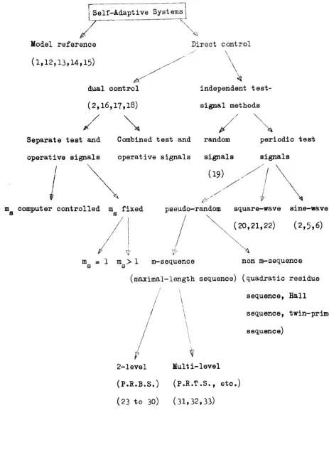
1.4 TYpes of Self-Adaptive Control Systems

10 11

There are many types of self~adaptive systems

'

, and these can

be classified in several different ways.

One class~fication

scheme is

outlined in figure

1.1.

To avoid confusion, the relationship bet-ween

parameters and performance index will be referred to as the 'plant', the

external controller being the 'system'.

Self-adaptive

systems can be divided into two main types:

Model reference

systems:,12,13,14,15.

_{These involve a two-fold}

process:

(a)

Model building, in which a model of the plant is

constructed,

either from variable analogue components

or as data in a digital computer.

The complexity of

the model is decided from an overall consideration of

the plant, and the values for the parameters are chosen

either offiline or by an on-line self-adaptive technique

~o give a performanoe as olose to that of the plant

as possible.

(b)

Pl~nt oontrol, in which the optimum values for the

parameters are calculated from the model, so that any

hill-climbing

is undertaken on the model and not

directly on the plant.

The plant parameters oan then

be adjusted accordingly.

The set-up is shown

---1

r:Lself-Adaptive

Systems \

//--

'",

IP

~

Model reference

Direct control

\

41

independent

test-(1,12,13,14,15)

_//

//.

b

dual control

(2,16,17,18)

signal methods

//

""~

Separate teat and

Combined test and

random

periodic test

operative signals

operative signals

J~

signals

signals

m

computer controlled

m

fixed

S

Ii!

~

m

>

I

s

pseudo-random

s~uare-wave

sine-wave

/

~

(20,21,22)

(2,5,6)

I

""

v,? ~

ID

=

1

s

m-se~uence

non m-se~uence

(maximal-length se~uence) (~uadratic residue

\

_{sequence, Hall}

\

se~uence, twin-prime

\

sequence)

\

I

\

[image:36.556.64.527.63.706.2]

2-1evel

Multi-level

(P.R.B.S. ) (P.R.T .S.,

etc.)

(23 to 30)

(31,32,33)

-·---1

rI-A ..

\.Ll :J

t;~

)--:) VI 0 Jr'

r

J

w

«

\-.

uJ

VI

et

r-VI

+~tC/\"

~

_

-- ~\U

v

o:

1:11 ~

Z

_j

0

l.w

\

_LJ

L

«

_J

,q

0

;l

::>

S

2:

~-

tf

j

-'

l

-

1-11

(ii) Direct Control Systems, in which no model of the plant is

explicitly used. _{Instead, the hill-qlimbing process is applied}

directly to the plant, by perturbing the parameters, deciding

whether this improves the performance or not, and changing the

operating point of the plant accordingly.

Direct control can be divided into two categories:

2 16 17 18

Dual-control' , , : in this case the test signal (the

exploratory parameter perturbation) is a step change, usually of

fixed magnitude, and the operative signal (the parameter change found

necessary to take the plant towards the optimum) is also a step, of

fixed or variable size. The method involves applying the test signal,

noting the change it produces in the performance, and choosing an

operative step accordingly. Each operative step can be used as

the subsequent test step, or the test and operative steps can be

distinct. In the latter Qase, the number of test steps to each

operative step, tn , Qan either be predetermined or be

computer-s

controlled during the QP~imization.

(i~

Independent test signal methods; in these systems, the test signal

is not a step, but is a signal with known statistical properties.

SU9h signals are classified in figure 1.7. These techniques are

all well-known, although the amount of comparative study work appearing

in the literature is small. For the most part, this thesis considers

methods using two types of test perturbation:

(a) sine-wave pertupbation2,5,6: the noise analysis of a sine-wave

~dentification techpique is given in Chapter

5.

(b) pseudo-random binary eequence

(P.R.B.S.,

or 'chain-code')

pert4D~ation23,24: the noise analysis of two

P.R.B.S.

identif-ication techniques is given in Chapters 2, 3 and 4, and the

design and performance of multi-parameter optimization systems

1-12

The optimization of plants having more than one dynamic path between

parameter and performance index is examined in Chapter

6

for both sine-wave

and chain-code perturbation systems. The performance of systems using

other oontrol techniques is disoussed in Chapter 10, where their relative

~erits are examined, and various strategies for rapid hill-climbing are

considered.

~.5

Chain-Codes

A brief description of the most signifioant properties of chain-codes

will now be given. A binary chain-code is a periodic signal which possesses

at any one time one of two states, and can switch from one state to the

other only at multiples of a basic interval,

>- ,

known as the clock-interval,

olock-time, or bit-interval. A chain~oode

is

oharacterized by the nature

of its auto-correlation funotion, defined by

¢cc('1:')==

J:

c(t) c(t -

't:)

dt •••••••••••••••••••••••••••••••• (

1.13)

where c(t) is the chain-code, T is its period, and ~ is the shift of one

code relative to the other. The 'pseudo-random' property of the

chain-oode implies that ¢cc(rr.) approximates to the auto-oorrelation function of

white noise, which is an impulse at zero shift. In fact

¢

(rr) consists

co

of a train of approximate impulses at intervals of T.

It is well-known that white noise can be applied to the input of a

plant as a test signal without it being correlated with other signals

occurring in the plant, and that the result of correlating the output of

the plant with the white noise gives the impulse response of the plant.

Using a chain-code as the test signal instead of the white noise yields

almos~ the same result, but has the advantage that the averaging time

needed for the oorrelation is finite, namely the chain-code period T.

1-13

1.6 The Experimental Facilities Used

The experimental work for this thesis was aided by the use of

three computing facilities:

(i) a G.E.C. 92 digital process-control computer

(ii) a Solartron 247 analogue computer

(iii) an Elliott 4130 digital data processing computer.

The G.E.C. 92 computer enables on-line computing to be carried out

on practical systems, or on models thereof. It has a memory of '8,000

l2-bit words; the most significant bit of each word is used to denote

sign, negative numbers being stored in two's complement form. The

word-length is adequate for most cont~ol problems, but double-length working can

be used if greater accuracy is required. The memory cycle time is

1.11~~

sec. Dig1tal-to-analogue and analogue-ta-digital converters are provided,

which can be switched to appropriate analogue lines by the programmer.

These lines come up on an interface connection panel, where they can either

be routed to other parts of the building, such as the engine test calls or

the fatigue laboratory, or linked directly to the analogue computer. Such

lines cap also be used for monitoriag purposes, using an oscilloscope or

graph~plotter.

The Solartron 241 Analogue Computer is used for simUlation of

praotical systems. It has facilities for multiplication and non-linear

function generating in addition to normal summing and integrating elements.

Facilities for iterative computation are provided, whereby successive

switching between the 'problem check', 'compute' and 'hold' modes can be

performed continuously, under the control of the internal timer or of

1-1 ~.

The Elliott 4130 computer is a high-speed data processing computer

for off-line calculations. The memory cycle-time has recently been

upgraded to

v=:

and the main-store capacity to 64,000 wo r-ds of

24-bits. There is also a magnetic tape backing store facility and a

graph--plot tar.

All these computing facilities have come into being during the

course of the work described in this thesis, some of which was compleied

before the computers became available. Some of the methods described

in the early part of the thesis can now be performed in the department

in a much simpler manner using the computers, but the methods are still

applicable in an environment where computers are not available or are

considered uneconomic for solving such problems. Considerable time

could however be saved, by replacing the tranGistori~ed circuits, such

as chain-code generators and running summers, by their integrated

circuit equivalents. Commercial ready-made equipment has come onto

the market recently which can perform some of the tasks of

code-generation and cross-correlation, but this equipment is very expensive

at present.

1.7 Aims and Contributions of the Thesis

When the work described in this thesis was started, the author

was invited to study two aspects of self-adaptive control using

chain-codes:

(i) The performance in the presence of noise of a particular

single-parameter system postulated in the literature.

(ii) The development of a multi-parameter optimizer which, it

was thought, might overcome the problems of interactions

between parameter paths, by using on-line esti~ates of the

interactions as correctionc for the gain estimates.

1-15

postulated could yield serious errors due to d.c. bias, even with no

noise present. As a result, an improved system was developed and

anslysed. Following on from this, an optimizer using sine-waves was

.analysed under noisy conditions and cbmpared with the chain- code

system. The application of each system to plants with single and

multiple dynamic paths between parameter and output was then examined.

Investigation into (ii) above showed that the suggested

compen-sation techniques will not work, and any similar methods would also

fail. Effort was then turned to the choice of multi-parameter optinizer

to give the best performance, in terms of short identification time,

small interaction errors and ease of implementation.

The contributions of this thesis can be summarized as:

(i) An exact mathematical analysis, supported by experimental

evidence, of the basic chain-code system, with and without

noise, with an assessment of the errors, and a design

procedure for choosing the parameters of the identification

Bystem.

(ii) The derivation of an improved system that overcomes the

major error of the original one •

.

(iii) Discussion of methods of implementing the improved system,

with and without recourse to a process-control computer.

(iv) Detailed analysis of the improved system, with and without

noise, yielding design criteria for the system, and showing

that the inherent errors in the system are not large enough

to prevent the system from being used as part of an optimizer.

Cv) .Analysis of the sine-wave system in the presence of noise,

and quantitative comparison with the improved chain-code system,

showing the benefits to be gained from each type of system.

1-16

show that errors arise in estimating the optimum of a plant

with parallel dynamic paths between parameter and output when

using sine-wave or chain-code perturbations.

"'~

(vii) Analysis of various compensation techniques for

multi-parameter identification, and a physical explanation of why

all such methods will fail.

,

(viii) A critical comparison of the methods described in the literature

for multi-parameter optimization.

(ix) Development of a method using shifted versions of one code

as parameter perturbations, for use with and without a

process-control computer.

(x) Realization of an on-line computer program for optimization

using shifted codes and a proportional-to-gradient optimization

strategy, with application to four-parameter plant moaels.

(xi) An analysis of the errors arising during optimization due

to the chanGing d.c. level of the plant output and to the

changing magnitude of the envelope of plant output values.

(xii) A survey of several of the available identification and

optimization techniques.

Although this thesis has been primarily concerned with

chain-code methods of optimization, it is not suggested that these are always

better than other techniques. In the last chapter it is shown that

some of the advantages of using chain-codes claimed in the literature,

such as good noise rejection and short identification time, do not

always survive after close examination. A quantitative comparison of

PART I

2-1

PART I:

SINGLFr-PARAMErER IDENTIFICATION

CRAnER

2

SINGLE-PARAMErER

IDENTIFICATION

USING CHAIN-CODES,

WITH AND WITHOUT NOISE PRESENT

2.1Introduction

In this chapter the performance of an identification system using

. 12 23 to 28

chain-oodes w11l be analysed ' • The system is based on the

well-known result (an extension of the Wiener-Hopf relation14) that states

that if a chain-code is applied to the input of a plant and cross-correlated

with the output, the resulting function, when scaled suitably, is

approximately the same as the impulse response of the plant. The

technique may be used to evaluate the gradient of the performance function

in an optimization loop47. In such a case, the parameter to be controlled

can be considered as the tinput' to the 'plant', and the output of the

performance function generator as the 'output' of the 'plant'. The gradi ent

of the performance function is then given by the gain from 'input' to 'output'

which can be deduced by integrating the impulse response to give the step

respon~e, and choosi.ng a value of this which is representative of its value

after an infinite time.

Th~ basic principle is described in Section 2.2. An alternative

method, using a running s~er (or averager), multiplier and integrator,

is desoribed and analysed under noise-free conditions in Section 2.3.

The practical implementation of the method is discussed, and experimental

results are given to support the theory. The behaviour of the system

under noisy conditions is ex~ined in Section 2.4. from theoretical and

2-2

2.2.The Basic Principle

It has been seen in Chapter 1 how a two-level chain-code is

charact~rised by having an auto-correlation function that approximates

to an impulse. If the code is applied to the input of a control system

and cross-correl~ted with the output,14,37,38,39 as shown in Figure

2.1,

the result is

¢

c/ 'l) =

.f

J:

c(t - '"t') Y

(t)

dt •••••••••••••••••••••••• (2.1)

where c(t) is a 'unit chain-code', that is, one having levels of + 1.

The convolution integral gives

y(t ) =

r:

u(

t -

s)

e

h(

s) ds •••••••••••••••••••••••••••••••• (

2.2)

where u(t)

=

ac(t), 'a' being a sgaling factor dictated by practical

considerations of the particular system to be identified. ('

s

I I.S c:.l.u ...tnj val"LQ.bk'

(Implicit in equation

(2.2)

is the assumption that h(~) is constant

with respect to time. For the present it will be assumed that the

charac~eristics of the plant are static.

If

this is not so, gh(~) must

be replaced by g(t)h('l:',t),making equation

(2.2)

difficult to manipulate.)

Substituting for yet) in equation

(2.1),

and l.nterchanging the order

of integration, gives

¢c/"l

=

~g [

¢

_cc('1:"-s) h(s) ds •••••••••••••••••••••• (2.3)

This is an exact relation. It will now be shown that, by making certain

approximations about

¢

("t),

¢

("'t') is proportional to the impulse

cc cy

response of the plant, h(s).

The approx~mation to be used is that given by equation

(Al.l.3)

of Appendix A1.l.

We

then have

N+l" [

a - Ag

N

0

S("'t"

-8)

h(a) ds

-.~-.-

---

..---.,--..._-•..-....-~~.--."-

--_

..,

-

...~.--.

,-~-~-~'---i

I

I

I '

I

_{1\ " __,,}

~~tj'

7)

-s:'

I

i

\

I

j /~'\

t~

I

i

I

__

~.

~__

l

---_,,.._---_._-

_.__

..

_-tJ

I

~~

(! ,

z.

I

:T oJ

\1.\

r'-

_I

<...P

I

z

r-dl

'VI

~ 0

I; )

I

"---"'

\

v')

V1

{l

U

\.d

cl

::J

\,1)

L_L

2-3

(Note that

LT

6('1:) d'1:' •

t.

ai nce the impulse can then be considered

to straddle the lower limit of integration, being equally disposed about it.

Sqme researchers have presented results where the first point of

¢ (~)

cy

has twice the value given above, which leads one to suspect their

technique, unless they have taken steps to double the value of

¢

(0)

cy

automatically. The resulting error in step response estimate is of course

very small.)

¢Cy

(L)

of the· plant.

is therefqre roughly proportional to the impulse response

An estimate of the step response at time T is given by

r

.i~tegrating this,

1\

S(Tr) ...

and scaling appropriately, so that

r

¢

("'t)

a-r ...•..

(2.5)

cy

N

whereas the true step response is

S(T

r)

•

t

Tr

s

h('t)

d't

(2.6)

The true gain of the system is given by

g :=

S(()C))

.•....•...

(2.7)

so that an estimate of gain is

. g = N

¢

_oy ('t") d"t"

If the impulse response has almost died away to zero in one period of

the cbam-code ,

foT

JI

h('t) d~~l •••••••••••••••••••••••••••••••••••••••••••••

'2.8)

80 ~hat ~ ::!:!::-' g •••••••••••••••••••••••••• ' ••••••••••••••••••••••••••••• (

2.9)

If the impulse response ~as a long settling time compared with the

ohain-code period, equation (2.8) cannot be deemed to hold. In addition

to this, errors will be brought forward from previous periods of the